Binaural Gain Modulation of Spectrotemporal Tuning in the Interaural Level Difference-Coding Pathway

Abstract

In the brainstem, the auditory system diverges into two pathways that process different sound localization cues, interaural time differences (ITDs) and level differences (ILDs). We investigated the site where ILD is detected in the auditory system of barn owls, the posterior part of the lateral lemniscus (LLDp). This structure is equivalent to the lateral superior olive in mammals. The LLDp is unique in that it is the first place of binaural convergence in the brainstem where monaural excitatory and inhibitory inputs converge. Using binaurally uncorrelated noise and a generalized linear model, we were able to estimate the spectrotemporal tuning of excitatory and inhibitory inputs to these cells. We show that the response of LLDp neurons is highly locked to the stimulus envelope. Our data demonstrate that spectrotemporally tuned, temporally delayed inhibition enhances the reliability of envelope locking by modulating the gain of LLDp neurons' responses. The dependence of gain modulation on ILD shown here constitutes a means for space-dependent coding of stimulus identity by the initial stages of the auditory pathway.

Introduction

The brainstem auditory system, an obligatory pathway for all aural information, must encode the location of a sound source, as well as its identity. Encoding information about spectrotemporal features is essential for discriminating between sounds, such as in speech and species-specific vocalizations (Shannon et al., 1995; Smith et al., 2002; Woolley et al., 2005; Suta et al., 2007; Nelson and Takahashi, 2010; Schneider and Woolley, 2010; Fogerty, 2011; Wang et al., 2011). In the auditory pathway, the timing of the spikes carries spectrotemporal information (Hermes et al., 1981; Theunissen et al., 2000; Escabí and Read, 2003; Linden et al., 2003; Joris et al., 2004; Christianson and Peña, 2007; Steinberg and Peña, 2011). This putative temporal code must be preserved with fidelity over several processing stages.

Barn owls localize sound sources using interaural time differences (ITDs) and interaural level differences (ILDs) (Konishi, 2003). In mammals and birds, these cues are processed in two parallel brainstem pathways (Schnupp and Carr 2009). In the barn owl, auditory nerve fibers bifurcate, one branch projecting to the cochlear nucleus angularis (NA) and the other to the cochlear nucleus magnocellularis (NM), giving rise to the ILD- and ITD-processing pathways, respectively (Sullivan and Konishi, 1984; Takahashi et al., 1984; Carr and Boudreau, 1991). Compared to NM neurons, NA neurons show enhanced ability to encode the stimulus envelope through increased sensitivity to power transients within their preferred frequency range (Steinberg and Peña, 2011; Kreeger et al. 2012). Thus, at the starting point of the ILD- and ITD-processing pathways, the former encodes the stimulus envelope with higher fidelity than the latter.

The posterior part of the lateral lemniscus (LLDp) is the first binaural nucleus in the ILD-processing pathway. Similar to cells in the mammalian lateral superior olive, cells here detect ILDs through the interplay of excitation and inhibition (Galambos et al., 1959; Boudreau and Tsuchitani, 1968). LLDp cells are excited by contralateral stimuli via NA and inhibited by ipsilateral stimuli via reciprocal connections from the LLDp of the opposite hemisphere (Manley et al., 1988; Takahashi and Konishi, 1988; Takahashi and Keller, 1992; Mogdans and Knudsen, 1994; Takahashi et al., 1995). This interplay of excitation and inhibition gives rise to sigmoid ILD tuning curves, where cells respond maximally to sounds that are louder in the contralateral ear.

Here we show how excitation and inhibition interact to enhance the fidelity of envelope locking in LLDp. Using binaurally uncorrelated noise, we measured the spectrotemporal receptive fields (STRFs) of the excitatory and inhibitory monaural inputs that converge onto LLDp neurons. We show that the balance of excitation and inhibition, which changes with sound location, modulates the gain of these neurons. This leads to greater response reliability of LLDp neurons to the stimulus envelope, meaning the reproducibility of precise spike timing across repeated presentations of a unique stimulus, compared to the last processing stage of the ITD pathway. This finding lends support to the hypothesis that the ILD pathway transmits spectrotemporal information to downstream structures with greater fidelity than the ITD pathway. In addition, our work suggests that sound source location may play a role in coding stimulus identity.

Materials and Methods

Surgery.

Data were collected from five adult barn owls (Tyto alba) bred in captivity. Since it is not possible to verify an owl's sex without invasive methods, sexes were undetermined. As described previously by Steinberg and Peña (2011), the birds were anesthetized by intramuscular injection of ketamine hydrochloride (20 mg/kg; Ketaset) and xylazine (4 mg/kg; Anased) over the course of the experiment. The depth of anesthesia was monitored by toe pinch. They also received an intramuscular injection of prophylactic antibiotics (oxytetracycline; 20 mg/kg; Phoenix Pharmaceuticals) and a subcutaneous injection of lactated Ringers solution (10 ml) at the beginning for each experiment. Body temperature was maintained throughout the experiment with a heating pad (American Medical Systems). A metal head plate was implanted at the beginning of the first recording session by removing the top layer of the skull and affixing it with dental cement while the head was held in stereotaxic position with ear bars and a beak holder. A small steel post was also implanted to demarcate a reference point for stereotaxic coordinates. Subsequently, all recording sessions were performed while the head was held in place by the head plate. A well was created on the skull around the stereotaxic coordinates for the LLDp, using dental cement, and the skin was sutured around it. A craniotomy was performed at the coordinates for the recording site, and a small incision was made in the dura mater for electrode insertion. At the end of a recording session, the craniotomy was sealed with Rolyan silicone elastomer (Sammons Preston). After the experiment, analgesics (ketoprofen, 1 mg/kg; Ketofen; Fort Dodge) were administered. Owls were returned to individual cages and monitored for recovery. These procedures comply with guidelines set forth by the National Institutes of Health and the Albert Einstein College of Medicine's Institute of Animal Studies.

Acoustic stimulation.

Dichotic stimulation was delivered in a double-walled sound-attenuating chamber (Industrial Acoustics). Custom software was used to generate stimuli and collect data. Earphones were constructed from a small speaker (model 1914; Knowles) and a microphone (model 1319; Knowles) in a custom-made aluminum case that fit the owl's ear canal. The microphones were calibrated using a Bruel and Kjaer microphone, allowing us to translate voltage output into decibels of SPL. The calibrated microphones were used to calibrate the earphones at the beginning of each experiment while inside the owl's ear canal. The calibration data contained the amplitudes and phase angles measured in frequency steps of 100 Hz. The stimulus generation software then used these calibration data to automatically correct irregularities in the amplitude and phase response of each earphone from 0.5 to 12 kHz (Arthur, 2004).

Acoustic stimuli consisted of broadband noise bursts with a linear rise and fall time of 5 ms.

Electrophysiology.

The LLDp was targeted by stereotaxic coordinates. Units were identified based on response properties unique to LLDp, which receives excitatory input from the contralateral NA and reciprocal inhibition from the contralateral LLDp (Fig. 1). Extracellular spikes were recorded from LLDp neurons using 1 MΩ tungsten electrodes (A-M Systems) and amplified by a DP-301 differential amplifier (Warner Instruments).

Figure 1.

Schematic depiction of the ILD-processing pathway with bilateral projections. The cochlear NA projects to the contralateral LLDp, as well as the contralateral ICcl. The LLDp nuclei of the two hemispheres reciprocally project to each other. LLDp also projects bilaterally to ICcl.

A spike discriminator (SD1; Tucker-Davis Technologies) converted neural impulses into TTL pulses for an event timer (ET1; Tucker-Davis Technologies), which recorded the timing of the pulses.

Data collection.

For each neuron we obtained rate-ITD, rate-ILD, and frequency tuning curves, as well as the monaural rate–intensity (RI) curve. ITD and ILD tuning curves were measured using 10 repetitions of 100-ms-long white-noise stimuli at randomly interleaved ITDs and ILDs. Frequency tuning curves were measured using 10 repetitions of 100 ms randomly interleaved pure tones between 500 Hz and 12 kHz presented at each neuron's best ILD. To estimate neurons' monaural RI curve, 10 repetitions of 100-ms-long white noise at sound levels from below threshold to saturation were presented in random order to the contralateral (excitatory) ear of each neuron (Table 1). To determine whether or not a neuron received inhibitory input from the ipsilateral ear, as opposed to just being excited by the contralateral ear, we performed the ILDf protocol, in which sound level is held fixed in the contralateral (excitatory) ear while varying the sound level in the ipsilateral (inhibitory) ear. Because LLDp neurons receive inhibitory input from the ipsilateral side, their response is depressed when the sound level in the ipsilateral ear reaches sufficient intensity (Manley et al., 1988). This protocol was performed with 100-ms-long noise bursts.

Table 1.

Overview of stimulation protocols

Stimulus protocol	Binaural vs monaural	Binaural correlation	Noise type	Sound level/ABI	ILD	Stimulus duration
ILD tuning curve	Binaural	100%	Unfrozen	Constant (40 dB)	−40 to 40 dB	100 ms
ILDf	Binaural	100%	Unfrozen	Varying	Varying	100 ms
Monaural intensity	Monaural	N/A	Unfrozen	10 dB to 80 dB	N/A	100 ms
STRF estimation	Binaural	0%	Unfrozen	Constant (40 dB)	2 ILDs over dynamic range	500 ms
Response reliability, ILD protocol	Binaural	100%	Frozen	Constant (40 dB)	2–3 ILDs over dynamic range	500 ms
Response reliability, ILDf protocol	Binaural	100%	Frozen	Varying	Varying	500 ms
Response reliability, monaural excitation protocol	Monaural	N/A	Frozen	2–3 dBs in dynamic range	N/A	500 ms

N/A, Not applicable.

Data used to determine the neurons' STRFs and their response reliability were collected as described previously (Christianson and Peña, 2007; Steinberg and Peña, 2011). Briefly, to measure binaural STRFs, we presented a string of de novo-synthesized broadband noise (unfrozen noise protocol). To measure neurons' monaural STRFs, binaurally uncorrelated noise stimuli were presented (Fischer et al., 2008). To measure response reliability, we used a “frozen noise” protocol, in which a single broadband noise stimulus (1 to 12 kHz) was repeated at different combinations of ILDs and sound levels (Table 1). Frozen noise stimuli were generated de novo each time this stimulus protocol was run, such that frozen noise tokens are unique for different instances of this protocol even for the same neuron. In all cases, noise segments were 500 ms long with a rise and fall time of 5 ms and at a stimulation rate of 1 stimulus per second or less.

Generalized linear model.

We used a generalized linear model (GLM) to describe spiking responses in LLDp (Paninski, 2004; Calabrese et al., 2011; Plourde et al., 2011; Fig. 2).

Figure 2.

Schematic description of the GLM model. Each ear's input is given by a spectrotemporal representation of the sound signal. Each ear's STRF is applied to the stimulus to give a weighted sum over frequency and time. The spike history kernel is a temporal filter applied to the spiking history to take into account refractory processes. The STRF-filtered stimuli are combined with the spike history and passed through a nonlinearity to produce an instantaneous firing rate. Spikes generated probabilistically with the instantaneous firing rate give rise to a predicted PSTH (red), which is compared to the neuron's response observed in vivo (black).

The response of the neuron is determined by the conditional intensity function λ(t|R(t)), where Prob(spike in [t, t + Δ]) ≈ λ(t|R(t))Δ for small time bins Δ.

The response of the neuron r(t) equals one if there is a spike and zero otherwise. The spike history, R(t), consists of the response at the previous K time steps: R(t) = [r(t − Δ), r(t − 2Δ), …, r(t − KΔ)].

The conditional intensity function is modeled such that spiking depends on (1) STRFs k_L and k_R applied to the left and right ear inputs s_L(t) and s_R(t), and (2) a spike history term k_spike that reflects refractory processes: λ[t|R(t)] = exp[k_L · s_L(t) + k_R(t) · s_R(t) + k_spike · R(t) + k₀] = exp[k_L · s_L(t)]exp[k_R · s_R(t)]exp[k_spike · R(t) + k₀].

Each ear's input is given by a spectrotemporal representation of the sound signal. The spectrotemporal representation of the sound is found by filtering the sound signal with a gammatone filter bank, computing the envelope of the output of each gammatone filter using the Hilbert transform, and taking the logarithm of the envelopes.

Each STRF is applied to one ear's input to give a weighted sum over frequency and time of the spectrotemporal input signal:

The spike history kernel is a temporal filter applied to the spiking history:

We used regularization to avoid overfitting. Regularization was incorporated into the model fitting procedure by adding a quadratic penalty on the model parameters to the log-likelihood of the data. Specifically, model parameters were found by maximizing the cost equal to L(k) − Q(k), where

is the log-likelihood of the data, and the quadratic penalty is given by the following:

The Matlab function glmfitqp (Mineault; Matlab Central) was used to find the parameters of the model that maximize the penalized log-likelihood of the observed spike response, binned at 0.5 ms.

We selected the scale parameters for the quadratic penalty η_i and the time and frequency ranges N and M for each neuron using cross-validation. We used responses to frozen, binaurally correlated noise bursts for cross-validation. In six neurons where the response to frozen noise was unavailable to use for cross-validation, we used a fivefold cross-validation. The cross-validation method tests the model by successively holding out a portion of the training data, fitting the model with the remaining data, and testing the model on the withheld data. This was done for five segments of the data set. A model peristimulus time histogram (PSTH) was generated over 10,000 trials, binned at 0.5 ms, and smoothed with a 5 ms Hanning window (Calabrese et al. 2011). The correlation coefficient between the model PSTH and the measured PSTH was used to assess the accuracy of the model.

STRF properties.

STRFs were described by the best frequency, frequency bandwidth, latency, and temporal bandwidth. The best frequency and latency were computed as the frequency and time, respectively, at the peak of the STRF. The frequency bandwidth was computed as the width at half-height of the frequency slice through the STRF at the latency. Similarly, the temporal bandwidth was computed as the width at half-height of the temporal slice through the STRF at the best frequency.

Characterizing gain modulation.

We characterized the gain modulation in the GLM output using responses of the model at two ILDs, one more inhibitory than the other, using the same frozen noise stimulus. The firing rate of the GLM is determined by the conditional intensity function f [x(t)], where the input to the model is x(t) = k_L · s_L(t) + k_R · s_R(t) + k_spike · R(t), and the STRFs and spike history kernel depend on ILD. We presented a frozen noise stimulus to the models at each ILD and measured the input signal x(t), averaged over trials, and the PSTH. We used linear regression to predict the input signal at the more inhibitory ILD x₁(t) from the input signal at the less inhibitory ILD x₂(t), as ax₂(t) + b. We then predicted the PSTH of the GLM at the inhibitory ILD using the input signal at the more excitatory ILD and the parameters of the linear regression as f (ax₂(t) + b). Because the input–output nonlinearity is the exponential function, this prediction can be rewritten as f [ax₂(t) + b] = exp[ax₂(t) + b] = exp(b)exp[ax₂(t)] = g₁f [g₂x₂(t)], where the gain parameters g₁ and g₂ depend on ILD, but not on the stimulus. Therefore, the GLM response at the small ILD is predicted by applying a gain to the input signal at the large ILD and to the input–output function of the GLM.

Response reliability.

The first 100 ms of each trial were excluded for the shuffled autocorrelogram (SAC), considering only those spikes that occurred once the firing rate had reached a steady state by visual inspection of the PSTH. In most neurons, this steady state was reached well before 100 ms after the stimulus onset in both frozen and unfrozen noise protocols.

Response reliability to the stimulus envelope was assessed by quantifying the reproducibility of the neural response to repeated presentations of the same stimulus using the SAC (Joris, 2003; Joris et al., 2006; Christianson and Peña, 2007; Steinberg and Peña, 2011). A spike train recorded during one presentation of the frozen noise stimulus is compared to all other spike trains recorded from other presentations of the same stimulus. For each possible combination, the forward time intervals are computed between pairs of spike trains using a 50 μs bin width. A normalizing factor was used, N(N −1)r²ΔτD, where r is the mean firing rate, Δτ is the bin width of the correlogram, and D is stimulus duration. This produces a unity baseline, where a spike train with Poisson statistics will have a flat SAC of height 1. The main parameter considered here to quantify neurons' response reliability is the height of this normalized SAC's peak at zero delay measured in number of normalized coincidences. This measure has also been referred to as the coincidence index.

To study how inhibitory drive influences response reliability, we used changes in firing rate as a proxy for changes in inhibitory input. We used three stimulation protocols: (1) the ILD protocol in which the average binaural intensity (ABI) was held constant while sounds were presented at two to three ILDs, (2) the ILDf protocol where sound level in the ipsilateral (inhibitory) ear was varied while keeping the sound level fixed at the contralateral (excitatory) ear, and (3) the monaural protocol in which sound level was varied in the contralateral (excitatory) ear without any sound presented to the ipsilateral (inhibitory) ear (Table 1). The combinations of ILDs, ABIs, and monaural intensity were chosen based on the dynamic range of each neuron. For the ILD and ILDf protocols, these values were chosen such that for one combination the neuron received minimum inhibitory drive. An additional one to two conditions were presented in which the neuron received a stronger inhibitory drive, but still produced enough spikes for SAC calculation. For the monaural stimulus protocol, intensities were presented such that a maximum firing rate was elicited, as well as two intensities around the center of the dynamic range, and another that elicited a lower firing rate. Since there is variation from neuron to neuron in spontaneous firing rate and dynamic range between stimulus protocols, we normalized changes in firing rate and response reliability (SAC peak height) for each neuron within each stimulus protocol to be able to compare across neurons. This resulted in what we call here the firing rate ratio (FR_rat) and SAC ratio (SAC_rat), defined as FR_rat = FR_ILDi/FR_ILDex and SAC_rat = SAC_ILDi/SAC_ILDex, where FR_ILDex and SAC_ILDex are the firing rate and SAC peak height, respectively, of conditions in the stimulus protocol at which the cell receives minimum inhibitory drive, and FR_ILDi and SAC_ILDi are the firing rate and SAC peak height of stimulus protocol conditions at which inhibitory drive is stronger. A similar calculation was conducted for the ILDf protocol, as well as the monaural stimulation protocol. We also repeated these calculations using the maximum firing rate across all stimulation protocols and its corresponding SAC peak as the denominator for FRrat and SACrat, as described above, as a control for biases introduced within conditions. Data were fit using a curve-fitting tool, the function cftool, in Matlab. Cftool performs several goodness-of-fit assessments, including sum of squares due to error, R₂, and root mean squared error. These measures were used to assess which was the best function form used to fit the data.

Linear regressions derived from these data were compared using a t test for the comparison of two slopes, as described by Zar (2009). This analysis algorithm is shown below, where the subscripts 1 and 2 denote data points from different data sets (in this case, two stimulus protocols, i.e., monaural vs binaural stimulation), and x and y denote FR_rat and SAC_rat data, respectively:

such that

and

where

Here, residual sum of squares (residual SS) and residual degrees of freedom (residual DF) are defined as follows:

and residual DF = n − 2, where n is the number of data points for each stimulus protocol.

Results

Our data set was obtained from 81 LLDp neurons recorded in five barn owls. LLDp neurons were targeted by stereotaxic coordinates and identified based on their response properties. LLDp neurons are unique within the auditory brainstem of the barn owl in that they are excited exclusively by sound in the contralateral ear, inhibited by the ipsilateral ear, narrowly tuned to frequency, and not tuned to ITD (Manley et al., 1988; Mogdans and Knudsen, 1994). To classify a neuron as belonging to the LLDp, all of these response properties were confirmed (Fig. 3). Therefore, LLDp cells can be distinguished from the cochlear nuclei, which respond to ipsilateral stimuli and from all other binaural nuclei in the region, tuned to ITD. Specifically, LLDp is located anatomically close to the anterior part of the dorsal lateral lemniscus, which exhibits robust ITD tuning; this prevents confusion of the two. Within the LLDp, there is an anatomical gradient of inhibitory input from dorsal to ventral, such that cells in the dorsal part of the nucleus receive significant inhibition, whereas cells in the most ventral part of the nucleus receive little inhibition (Manley et al., 1988; Takahashi et al., 1989; Takahashi and Keller, 1992). Thus, most LLDp cells are inhibited when sound is increased in the ipsilateral ear while holding the sound level constant in the contralateral (excitatory) ear.

Figure 3.

Example of response properties of four LLDp neurons. Each row represents one neuron. A–D, Rate-ITD curves. (These neurons are not tuned to ITD.) E–H, Rate-ILD curves. I–L, Isointensity frequency-tuning curves. M–P, Rate-ILDf curves, where sound level was held constant in the contralateral (excitatory) ear while it was varied in the ipsilateral (inhibitory) ear as indicated on the x-axis. Neurons in the first three rows were recorded from the left hemisphere, while the neuron recorded in the last row was recorded from the right hemisphere. Therefore, the ILD curve in the last row is reversed relative to the other neurons. Error bars indicate SEM.

STRFs of LLDp cells

We estimated the STRFs of 40 LLDp neurons using a point process model of LLDp spiking responses. As demonstrated previously in the barn owl's nucleus laminaris (Fischer et al., 2008; Fischer et al., 2011), binaurally uncorrelated noise can be used to study the monaural inputs of auditory neurons. We used this strategy in LLDp neurons to estimate the STRFs of the excitatory, contralateral (eSTRF) and the inhibitory, ipsilateral (iSTRF) monaural inputs. Unlike the tuning to ITD in the nucleus laminaris, cells in LLDp become tuned to ILD through interaction of contralateral excitatory and ipsilateral inhibitory inputs (Manley et al., 1988; Takahashi and Keller, 1992; Mogdans and Knudsen, 1994; Takahashi et al., 1995). Thus, this method allowed us to compute the STRF of the inhibitory input that LLDp neurons receive from the contralateral LLDp and compare it to the STRF of the excitatory input.

We fit a GLM of 40 LLDp neurons using their responses to binaurally uncorrelated sounds. The GLM describes the spiking probability as a nonlinear function of a linear combination of the monaural filter outputs, and a spike history term that models refractory processes (Paninski 2004; Calabrese et al. 2011; Plourde et al., 2011). These STRFs were cross-validated with the responses of 34 of these neurons to frozen noise. The mean correlation between the response to frozen noise and the predicted response from monaural STRFs was 0.58 ± 0.18. The eSTRFs best frequency (eSTRF_bf) ranged from 1.2 to 8 kHz. The best frequencies of eSTRFs and iSTRFs (iSTRF_bf) were strongly correlated (iSTRF_bf = eSTRF_bf + 7 Hz, r = 0.96, p < 0.001, Fig. 4A). The median eSTRF bandwidth was 867 Hz, and the median eSTRF temporal width was 1.47 ms. The median iSTRF bandwidth was 976 Hz; this did not differ significantly from eSTRFs (Kruskal–Wallis test, p > 0.05; Fig. 4B). The median iSTRF temporal width was significantly broader than the eSTRF temporal width at 1.85 ms (Kruskal–Wallis test, p < 0.001; Fig. 4C). The median latency of the inhibitory minimum, 6.49 ms, was significantly longer than that of the excitatory maximum at 5.47 ms (Kruskal–Wallis test, p < 0.001; Fig. 4D).

Figure 4.

Comparison of monaural excitatory and inhibitory STRF properties. A, eSTRFbf and iSTRFbf were strongly correlated (iSTRF_bf = eSTRF_bf + 7 Hz, r = 0.96, p < 0.001). B, Distribution of differences in bandwidth (bw) shown as cell counts. iSTRFbw was not significantly broader than eSTRFbw (Kruskal–Wallis test, p > 0.05). C, Distribution of differences in temporal width (tw) shown as cell counts. iSTRFtw was significantly larger than eSTRFtw (Kruskal–Wallis test, p < 0.001). D, Distribution of differences in STRF latency shown as cell counts. The latency of inhibitory STRFs was significantly longer than that of excitatory STRFs (Kruskal–Wallis test, p < 0.001).

The difference in latency between excitation and inhibition is consistent with inhibition arriving at LLDp via two synapses (Takahashi and Konishi, 1988; Takahashi and Keller, 1992; Takahashi et al., 1995), while excitation must only traverse one synapse, resulting in a built-in delay. In addition, the latency of excitation and inhibition relative to each other varies with ILD, as the latency of the neural response becomes shorter with increasing sound levels (Aitkin et al., 1970). Thus, as ILD changes, the sound levels at both the excitatory and inhibitory ears change, leading to opposite shifts in latency in both inputs. To measure inhibitory STRFs, ILDs that elicited both excitation and inhibition were used. Most of the data were obtained at small ILDs, at which sound levels at the two ears are similar. Large ILDs favoring the inhibitory side prevent the neuron from firing. At large ILDs favoring excitation, sound levels are much higher in the excitatory ear and comparatively low in the inhibitory ear, leading to a decrease in the latency of excitation and an increase in the latency of inhibition.

Response reliability in LLDp

We next studied the effect of inhibition on the response reliability to repeated broadband noise stimuli (frozen noise). Because the inhibitory input to these cells is driven by sound presented to the ipsilateral ear while excitation is driven by sounds in the contralateral ear, the effect of inhibition on response reliability can be assessed by varying sound levels in the inhibitory ear, excitatory ear or both. Changes in firing rate were used as a proxy for the amount of inhibition. Firing-rate changes were normalized across the population by computing changes in firing rate as the ratio of firing rates at different ILDs. We examined the relationship between FR_rat and the corresponding ratio of changes in the normalized SAC peak heights (SAC_rat).

First, we presented frozen noise at different ILDs. Representative rasters are shown in Figure 5A–C. For each cell, we chose the largest excitatory ILD that elicited the maximum firing rate as the denominator in the FR_rat. Decreasing ILD, i.e., increasing the sound level on the inhibitory input while decreasing the sound level on the excitatory input, causes a decrease in firing rate. ILDs for which the inhibitory input was louder than the excitatory input usually abolished the response. Thus, to measure the effect of inhibition, we presented sound at an ILD in the center of the neuron's dynamic range and an ILD that elicited a lower firing rate but still sufficient to calculate STRFs and SACs. The mean percentage suppression of firing rate was 45 ± 25%. We found that response reliability increased as the inhibitory drive became stronger (Fig. 5D,E). There was a power-law relationship between the FR_rat and its corresponding SAC_rat (Fig. 5F; y = 1.09x^−0.55, r² = 0.54, n = 51).

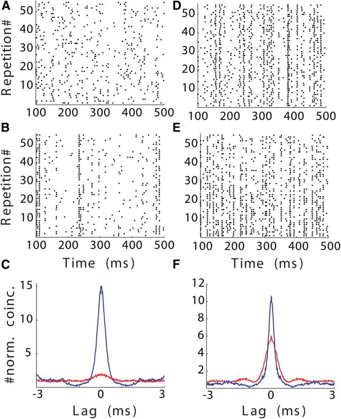
Figure 5.

Inhibition enhances response reliability. A–C, Representative rasters of one neuron recorded at an ILD that induced minimal (ILD, 20 dB; A), intermediate (ILD, 10 dB; B), and maximal suppression (ILD, 0 dB; C). D, Overlapped PSTH excerpts of responses depicted in A–C at ILD 20 dB (red), ILD 10 dB (black), and ILD 0 dB (blue). E, Normalized SACs for ILD 20 dB (red), ILD 10 dB (black), and ILD 0 dB (blue). F, Overlapped data comparing the relationship of normalized SAC peak ratios to corresponding firing rate ratios for changing ILDs (filled circles, dashed line; y = 1.09x^−0.55, r² = 0.54, n = 51) and monaural stimulation at different sound levels (triangles, solid line; y = −0.81x + 1.78, r² = 0.25, n = 38). Data points from the neuron in this figure are highlighted in red. Note that for similar relative decreases in firing rate, proportional changes in response reliability tend to be greater in the presence of inhibition.

To control for the effects of change in excitatory drive on response reliability, we performed two further experiments. First, we presented frozen noise keeping the sound level in the excitatory ear constant and varying the sound level in the inhibitory ear alone (ILDf curve). The mean percentage suppression of firing rate was 28.1 ± 24%. Again we found a power-law relationship between FR_rat and SAC_rat (y = 0.92x^−0.67, r² = 0.71, n = 25). Next, we presented frozen noise with varying sound levels in the excitatory ear alone with no sound in the inhibitory ear. The mean reduction in firing rate was 40 ± 25%. This yielded an inverse relationship between FR_rat and SAC_rat (Fig. 5F; y = −0.81x + 1.78, r² = 0.25, n = 38).

To be able to statistically compare these relationships, we converted all data points to a log scale, which allowed us to compare all three stimulus protocols as linear regressions (ILD, y = −0.57x +0.01, r² = 0.61; ILDf, y = −0.58x + 0.06, r² = 0.45; monaural, y = −0.24x + 0.07). We found that both the ILD and ILDf protocol regressions differed significantly from the monaural excitatory protocol regression (t test, p < 0.001). The ILD and ILDf protocol regressions did not differ significantly from each other (t test, p > 0.1).

These analyses were repeated for a subset of neurons from which both monaural excitatory as well binaural excitatory recordings were available (n = 14). Here, we normalized the neurons' firing rate and SAC peak heights by the maximum firing rate observed across all stimulus protocols and its corresponding SAC peak height. The results mirrored those above in that binaural stimulus protocols (ILD, ILDf) yielded a power-law relationship between firing rate and SAC peak height (y = 1.1x^−0.58, r² = 0.66), while monaural stimulation yielded a linear relationship (y = −0.8x +1.78, r² = 0.33). When converted to log scale, the monaural excitatory data yielded a regression described by y = −0.25x + 0.06, while the binaural protocol data yielded a regression described by y = −0.63x − 0.04. These regressions are significantly different (t test, p < 0.001).

As a further control, we compared normalized SAC peak heights between binaural and monaural stimulation in a subset of cases where firing rates were within 10% of each other (n = 7; Fig. 6). Here we chose conditions that elicited firing rates of 50% or below the maximal firing rate for these neurons to guarantee that in the binaural cases inhibition was present. The 50% value was chosen as an arbitrary cutoff based on the observation that the effect of inhibition on response reliability becomes more prominent at FR_rat < 0.5 (Fig. 5F). The SAC peak height was normalized by the SAC peak observed at each neuron's maximum firing rate across all stimulus protocols (SAC_rat). We found that normalized SAC peak heights were significantly larger in the presence of inhibition compared to excitation alone (monaural, 1.17 ± 0.56; binaural, 2.5 ± 1.73; Kruskal–Wallis test, p < 0.001).

Figure 6.

Comparison of monaural and binaural data matched for firing rate for two neurons. A, Raster of spikes triggered during monaural presentation of repetitions of the same unique stimulus. Mean FR is 21.4 spikes/s. B, Raster of spikes triggered during binaural repetition of a second unique stimulus for the same neuron shown in A. Mean FR is 19.5 spikes/s. C, Overlapped SACs for monaural (red) and binaural (blue) stimulation protocols for the same cell as in A and B. D–F, Same configuration as in A–C for a second neuron. C, FR is 39.8 spikes/s. D, FR is 40.8 spikes/s. Note that because sound tokens in A and B and D and E were different, spiking patterns differ across rasters.

These data indicate that inhibition has a significant effect enhancing response reliability, beyond the effect of firing rate modulation induced by changes in excitatory drive alone. This suggests that excitation and inhibition interact in a nonlinear fashion to modulate the gain of spectrotemporal tuning (addressed in the next section).

We compared the SAC measurements to previously published data from the central core of the inferior colliculus (ICcc), the last nucleus belonging exclusively to the ITD-coding pathway (Christianson and Peña, 2007). We found that at ILDs that elicited a maximal firing rate in LLDp, there was no significant difference in response reliability between NA and ICcc (median SAC peak values, LLDp, 3.34; ICcc, 3.74; NA, 4.3; Kruskal–Wallis test, p > 0.3). However, for ILDs at which inhibitory drive was present, response reliability in LLDp was significantly greater in LLDp than ICcc (LLDp median SAC peak, 6.11; Kruskal–Wallis test, p < 0.03). These data support our hypothesis that the ILD-processing pathway transmits spectrotemporal information with greater fidelity to structures in the midbrain and forebrain than the ITD-processing pathway.

ILD-dependent gain modulation

For 19 neurons, we recorded data to fit the GLM at two ILDs (Fig. 7). For those neurons with significant STRFs at both ILDs, the main features of the STRFs including best frequency, bandwidth, latency, temporal width, and peak amplitude did not change significantly when ILD changed (n = 15; two-sample Kolmogorov–Smirnov test, all p ≥ 0.05; Fig. 7A–D,K–N). For four neurons, the inhibitory STRF was not significant at the most excitatory ILD, but emerged at the smaller ILD. The constant bias of the GLM k₀ also did not change significantly with ILD (two-sample Kolmogorov–Smirnov test, p = 0.74; Fig. 7E,O). The spike history kernels were also similar across changes in ILD (correlation coefficient, 0.87 ± 0.15; Fig. 7F,P). We fit each spike history kernel with an exponential function, and the amplitude and time constant of the exponential fits were not significantly different between the two ILDs (n = 19; two-sample Kolmogorov–Smirnov test, p ≥ 0.74 for both). Thus, there was no consistent difference between the component parameters of the GLMs at the two ILDs. However, the overall change in the GLM response with ILD that was consistent across all neurons was a gain modulation.

Figure 7.

Gain modulation of spectrotemporal selectivity as ILD changes. Examples of the generalized linear model at two ILDs for two neurons and the model responses to frozen noise. Here ILD changes by increasing sound level in the inhibitory ear and decreasing sound level in the excitatory ear. A–F, K–P, The model components show the eSTRFs (left) and iSTRFs (right) for a large ILD (A, B, K, L) and a small, more inhibitory ILD (C, D, M, N). The remaining model components are the constant bias (E, O) and the spike history kernels (F, P). G–J, Q–T, The responses of the models to frozen noise on the right reveal an ILD-dependent gain modulation. G, Q, The rate responses (spikes per trial in 0.5 ms time bins) of the models at an ILD that induced weaker inhibition (red) and an ILD eliciting stronger inhibition (blue) show peaks at similar times. H, R, The input–output functions of the models at the ILDs with (blue circles) and without (red squares) inhibition are similar exponentials, but the inputs lie in different regions. I, J, S, T, Applying a gain modulation to the input at the ILD without inhibition (red) predicts the response to the more inhibitory ILD (blue).

Increasing inhibition by changing ILD resulted in an overall gain decrease in the firing rate of the neuron. For a frozen noise stimulus, the STRF-filtered input was very similar across ILDs, but there was a change in the gain of the signal (correlation coefficient, 0.93 ± 0.07). Correspondingly, the PSTH of the model response were similar across ILDs, but there was a change in gain (correlation coefficient, 0.78 ± 0.13; Fig. 7G,I,Q,S). The mean firing rate of the GLM was significantly lower at the more inhibitory ILD (Kruskal–Wallis test, p = 0.003).

The GLM responses to frozen noise at the two ILDs were related by a gain modulation. The PSTHs of the GLM responses at the two ILDs showed peaks at the same time points, but the response at the more inhibitory ILD was reduced relative to the response at the other (Fig. 7G,Q). The firing rate of the GLM is determined by passing an input signal through an input–output nonlinearity f [x(t)], where the input signal consists of the STRF-filtered stimulus and the filtered spike history. Because of the high correlation of the STRF-filtered stimulus across ILDs, it was possible to predict the PSTH at the more inhibitory ILD using a gain-modulated version of the input stimulus at the more excitatory ILD of the form g₁f[g₂x(t)], where a constant gain is applied to the input signal at the excitatory ILD and to the input–output nonlinearity (Fig. 7H,J,R,T; correlation coefficient, 0.78 ± 0.12; see Materials and Methods). These data support the conclusion that spectrotemporal tuning is robust to changes in ILD and that increasing inhibition produces a decrease in neural gain.

To confirm that the gain modulation was an effect of inhibition alone and not of the decrease in excitation induced by changing ILD, we modified the stimulation protocol such that the intensity of the excitatory side was kept constant and only the inhibitory side was changed (ILDf curve). As before, model responses in the two conditions were related by a gain modulation. The correlation between the PSTH at the more inhibitory ILD and the rescaled prediction was high (Fig. 8; correlation coefficient, 0.82 ± 0.09; n = 7).

Figure 8.

Gain modulation of spectrotemporal selectivity as inhibition increases. Examples of the generalized linear model at two ILDs and the model responses to frozen noise. Here ILD changes by increasing sound level in the inhibitory ear while keeping constant the sound level in the excitatory ear. Plots are as in Figure 7.

Visual inspection of rasters and PSTHs recorded in vivo similarly showed that, despite variations in firing rate, cells tended to fire spikes at the same time at different ILDs (Fig. 5D). This supports data from the GLM model that suggest that inhibition does not qualitatively change the spectrotemporal tuning of LLDp cells, but mainly acts to scale responses to spectrotemporal features divisively. To quantify this observation, we calculated the correlation coefficient of the PSTHs for the same stimulus at different ILDs in each cell. The mean correlation coefficient was 0.54 ± 0.21 (p < 0.05; n = 50) binned at 1 ms. Discrepancies between PSTHs at different ILDs were generally due to decreased spike counts in low-probability bins. This confirms the model's prediction that as inhibitory drive increases and the gain of LLDp neurons decreases, their responses become more selective to spectrotemporal features. Interestingly, the largest peaks in PSTHs did not always correspond across ILDs. Similar effects have been observed in the primary visual cortex under condition of nonclassical receptive field stimulation in conjunction with classical receptive field stimulation, as well as during natural scene presentation (Vinje and Gallant, 2000; Haider et al., 2010).

Discussion

Here we study how inhibition enhances the reliability of the response to spectrotemporal features of LLDp neurons, the first site of binaural convergence of excitatory and inhibitory inputs in the owl's auditory pathway. These data support previous work in the lateral geniculate nucleus (Butts et al., 2011) as well as previous reports from the auditory cortex (Wehr and Zador, 2003; Wu et al., 2008) and somatosensory cortex (Gabernet et al., 2005; Wilent and Contreras, 2005) that suggest that delayed inhibition can enhance stimulus selectivity, spike-timing precision, and reliability. Our work supports the notion that this is a general mechanism in sensory coding, across stages and species. Our data are unique in that the circuit studied anatomically and functionally separates excitatory and inhibitory inputs to the neurons. This allowed us to clearly delineate the contribution and tuning of the two inputs.

Gain modulation has been studied in a variety of systems, and it has been found that excitation and inhibition act on the input–output function of neurons in a complex manner (Andersen et al., 1985; Chance et al., 2002; Mitchell and Silver, 2003; Murphy and Miller, 2003; Prescott and De Koninck, 2003; Cardin et al., 2008; Ly and Doiron, 2009). The gain modulation effects of inhibition have generally been described in conjunction with noise in the subthreshold membrane potential or the input (Chance et al., 2002; Mitchell and Silver, 2003; Murphy and Miller, 2003; Prescott and De Koninck, 2003; Ly and Doiron, 2009). This is consistent with our data, where the responses of neurons to spectrotemporal features exhibit a fair amount of noise due to both the intrinsic variability of the signal used as stimulus as well as the noisy spike generation. A previous modeling paper by Gittelman et al. (2012) showed that FM selectivity of neurons in the inferior colliculus of the bat may be accounted for by gain modulation via inhibition, which promotes more selective spiking activity. This, too, is consistent with our data, which demonstrate that inhibitory drive exerts divisive gain modulation in LLDp neurons, which decreases spikes fired in low-spiking-probability time bins. Effectively, this leads to greater reliability of these neurons' responses to spectrotemporal features.

Because ILD varies with sound direction, the neurons' gain can be modulated by the spatial location of a stimulus. This mechanism may be useful in auditory scene analysis by adding another dimension to envelope coding (Nelken, 2004). Previous data from Field L, the avian equivalent of auditory cortex, show that the neurons' responses to birdsong may be modulated by spatial location when presented together with a masking sound (Maddox et al., 2012). Interestingly, the influence of spatial location of a sound source was weak in the absence of a masking sound, possibly speaking to the relationship between noise in subthreshold membrane potentials and gain modulation. Our data provide an example of gain modulation at an earlier stage in the auditory processing stream and address how inhibition mechanistically could account for this observation at the level of the brainstem.

The role of stimulus context in gain control has been studied in both the visual and auditory systems. In the visual system, neurons' gain is modulated by contrast (Shapley and Victor, 1981). Andersen et al. (1985) showed that the responses of posterior parietal cortex neurons were gain modulated by gaze angle. Gain modulation is also dependent on the spatiotemporal properties of visual stimuli (Cardin et al., 2008). In the auditory cortex, contrast has been shown to modulate gain (Rabinowitz et al., 2011). Winkowski and Knudsen (2006) showed that top-down gain control modulates responses of neurons in the auditory midbrain, suggesting that attention may play a role.

Another novel aspect of our data set is the relationship between gain modulation and response reliability. A study in the primary visual cortex demonstrated previously that extraclassical receptive field stimulation increases inhibitory postsynaptic potentials, leading to increased reliability of excitatory postsynaptic potentials and spikes (Haider et al., 2010). However, this was not related to gain modulation, as we were able to do in our study. Data from the auditory cortex have shown that combinations of excitation and inhibition with similar spectral tuning could lead to downstream sharpened tuning (Wehr and Zador, 2003; Wu et al., 2008). This may underlie increased spike-timing precision. Our work shows that while spectrotemporal tuning is invariant to the level of excitation and inhibition, inhibition enhances selectivity through gain modulation of the input–output function. This, in turn, leads to enhanced response reliability.

At the cochlear nuclei NM and NA, we found that NA neurons encoded spectrotemporal information with higher fidelity (Steinberg and Peña, 2011). We related this observation to specific attributes of NA cells spectrotemporal tuning, apparent in their STRFs. We found that the greater the magnitude of the suppressive field in NA neurons' STRFs, the greater their response reliability, a measure of their ability to lock to the stimulus envelope. This study examines whether this difference in fidelity of spectrotemporal coding observed between NA and NM is maintained in later processing stages within the sound localization pathways. We show that at the final processing stages of the ILD and ITD pathways, the ILD coding pathway responds to spectrotemporal features with higher fidelity than the ITD pathway.

Mogdans and Knudsen (1994) reported on the discharge pattern of LLDp neurons. Several of their qualitative observations agree with our findings. First, they observed that as sound level in the ipsilateral ear was increased, some spikes during the sustained response disappeared while others remained. Furthermore, spike timing under conditions of strong inhibition was more patterned than when a similar firing rate was elicited by weak excitation only. They showed that while monaural excitatory and binaural stimuli elicited similar firing rates during the onset of the response, the sustained portion of the response exhibited a much lower firing rate during binaural stimulation. This may be due to a temporal delay in the arrival of inhibition at LLDp neurons, thereby shielding the onset of neurons' response. These data support our decision to exclude response onsets from our analysis, by indicating that inhibition most robustly affects the sustained component of the response.

Manley et al. (1988) demonstrated the role of inhibition in the detection of ILD and suggested that excitation and inhibition may be matched in best frequency. It was later shown that the inhibitory drive originated in the contralateral LLDp (Takahashi and Keller, 1992; Takahashi et al., 1995). Takahashi et al. (1995) supported the notion that excitation and inhibition were matched in best frequency, based on the observation that projections from one LLDp targeted the same tonotopic region in the contralateral LLDp. Here we confirm this observation, as inhibitory and excitatory monaural STRF_bf values are highly correlated.

LLDp cells project to the lateral shell of the inferior colliculus (ICcl), which also receives input from the ICcc, the last stage of the ITD-processing pathway, and NA. Previous work has demonstrated that cells in ICcl lock well to stimulus envelope with modulation rates of up to 100 Hz (Keller and Takahashi, 2000). Christianson and Peña (2007) demonstrated that neurons in NL, the site of binaural convergence in the ITD-processing pathway, and ICcc also lock to the stimulus envelope, albeit with less reliability than observed in LLDp. It has been suggested previously that the ILD pathway may be responsible for transmitting envelope information to ICcl (Keller and Takahashi, 2000; Steinberg and Peña, 2011). Our data support this hypothesis, as the output of LLDp to ICcl exhibits high-fidelity envelope locking.

It has been suggested that inhibition plays a critical role in encoding and discriminating complex sounds (Narayan et al., 2005; Woolley et al., 2005; Andoni et al., 2007; David et al., 2009; Ye et al., 2010). Inhibition of broader spectral tuning than excitation has been involved in shaping frequency-sweep direction selectivity (Zhang et al., 2003; Kuo and Wu 2012). Moreover, it has been shown that the spectrotemporal profile of the inhibitory drive changes when different types of stimuli are used (Woolley et al., 2005; David et al., 2009). Our work demonstrates that delayed, spectrotemporally tuned inhibition enhances envelope locking by gain control, leading to the suppression of low-probability responses. This is important to the discrimination of complex stimuli, such as speech, whose intelligibility has been shown to rely heavily on envelope information (Shannon et al., 1995; Smith et al., 2002; Fogerty, 2011).

In summary, we demonstrate that neurons in the last stage of the owl's ILD-processing pathway, the nucleus LLDp, encode spectrotemporal features with higher fidelity than the last nucleus of the ITD-processing pathway. Inhibition acts on the LLDp neurons to modulate the gain of the input–output function, which leads to decreased number of spikes in low-probability time bins and increased reliability of envelope locking. Response reliability increases for ILDs where inhibition becomes stronger, yielding a space-dependent gain modulation that enhances envelope locking along the dynamic range of the cells. This gain modulation may constitute an early feedforward mechanism to enhance the reliability of spectrotemporal coding.

References

- Aitkin LM, Anderson DJ, Brugge JF. Tonotopic organization and discharge characteristics of single neurons in nuclei of the lateral lemniscus of the cat. J Neurophysiol. 1970;33:421–440. doi: 10.1152/jn.1970.33.3.421. [DOI] [PubMed] [Google Scholar]
- Andersen RA, Essick GK, Siegel RM. Encoding of spatial location by posterior parietal neurons. Science. 1985;230:456–458. doi: 10.1126/science.4048942. [DOI] [PubMed] [Google Scholar]
- Andoni S, Li N, Pollak GD. Spectrotemporal receptive fields in the inferior colliculus revealing selectivity for spectral motion in conspecific vocalizations. J Neurosci. 2007;27:4882–4893. doi: 10.1523/JNEUROSCI.4342-06.2007. [DOI] [PMC free article] [PubMed] [Google Scholar]
- Arthur BJ. Sensitivity to spectral interaural intensity difference cues in space-specific neurons of the barn owl. J Comp Physiol A. 2004;190:91–104. doi: 10.1007/s00359-003-0476-1. [DOI] [PubMed] [Google Scholar]
- Boudreau JC, Tsuchitani C. Binaural interaction in the cat superior olive S segment. J Neurophysiol. 1968;31:442–454. doi: 10.1152/jn.1968.31.3.442. [DOI] [PubMed] [Google Scholar]
- Butts DA, Weng C, Jin J, Alonso JM, Paninski L. Temporal precision in the visual pathway through the interplay of excitation and stimulus-driven suppression. J Neurosci. 2011;31:11313–11327. doi: 10.1523/JNEUROSCI.0434-11.2011. [DOI] [PMC free article] [PubMed] [Google Scholar]
- Calabrese A, Schumacher JW, Schneider DM, Paninski L, Woolley SM. A generalized linear model for estimating spectrotemporal receptive fields from responses to natural sounds. PLoS One. 2011;6:e16104. doi: 10.1371/journal.pone.0016104. [DOI] [PMC free article] [PubMed] [Google Scholar]
- Cardin JA, Palmer LA, Contreras D. Cellular mechanisms underlying stimulus-dependent gain modulation in primary visual cortex neurons in vivo. Neuron. 2008;59:150–160. doi: 10.1016/j.neuron.2008.05.002. [DOI] [PMC free article] [PubMed] [Google Scholar]
- Carr CE, Boudreau RE. Central projections of auditory nerve fibers in the barn owl. J Comp Neurol. 1991;314:306–318. doi: 10.1002/cne.903140208. [DOI] [PubMed] [Google Scholar]
- Chance FS, Abbott LF, Reyes AD. Gain modulation from background synaptic input. Neuron. 2002;35:773–782. doi: 10.1016/S0896-6273(02)00820-6. [DOI] [PubMed] [Google Scholar]
- Christianson GB, Peña JL. Preservation of spectrotemporal tuning between the nucleus laminaris and the inferior colliculus of the barn owl. J Neurophysiol. 2007;97:3544–3553. doi: 10.1152/jn.01162.2006. [DOI] [PMC free article] [PubMed] [Google Scholar]
- David SV, Mesgarani N, Fritz JB, Shamma SA. Rapid synaptic depression explains nonlinear modulation of spectro-temporal tuning in primary auditory cortex by natural stimuli. J Neurosci. 2009;29:3374–3386. doi: 10.1523/JNEUROSCI.5249-08.2009. [DOI] [PMC free article] [PubMed] [Google Scholar]
- Escabí MA, Read HL. Representation of spectrotemporal sound information in the ascending auditory pathway. Biol Cybern. 2003;89:350–362. doi: 10.1007/s00422-003-0440-8. [DOI] [PubMed] [Google Scholar]
- Fischer BJ, Christianson GB, Peña JL. Cross-correlation in the auditory coincidence detectors of owls. J Neurosci. 2008;28:8107–8115. doi: 10.1523/JNEUROSCI.1969-08.2008. [DOI] [PMC free article] [PubMed] [Google Scholar]
- Fischer BJ, Steinberg LJ, Fontaine B, Brette R, Pena JL. Effect of instantaneous frequency glides on interaural time difference processing by auditory coincidence detectors. Proc Natl Acad Sci U S A. 2011;108:18138–18143. doi: 10.1073/pnas.1108921108. [DOI] [PMC free article] [PubMed] [Google Scholar]
- Fogerty D. Perceptual weighting of individual and concurrent cues for sentence intelligibility: frequency, envelope, and fine structure. J Acoust Soc Am. 2011;129:977–988. doi: 10.1121/1.3531954. [DOI] [PMC free article] [PubMed] [Google Scholar]
- Gabernet L, Jadhav SP, Feldman DE, Carandini M, Scanziani M. Somatosensory integration controlled by dynamic thalamocortical feed-forward inhibition. Neuron. 2005;48:315–327. doi: 10.1016/j.neuron.2005.09.022. [DOI] [PubMed] [Google Scholar]
- Galambos R, Schwartzkopff J, Rupert A. Microelectrode study of superior olivary nuclei. Am J Physiol. 1959;197:527–536. doi: 10.1152/ajplegacy.1959.197.3.527. [DOI] [PubMed] [Google Scholar]
- Gittelman JX, Wang L, Colburn HS, Pollak GD. Inhibition shapes response selectivity in the inferior colliculus by gain modulation. Front Neural Circuits. 2012;6:67. doi: 10.3389/fncir.2012.00067. [DOI] [PMC free article] [PubMed] [Google Scholar]
- Haider B, Krause MR, Duque A, Yu Y, Touryan J, Mazer JA, McCormick DA. Synaptic and network mechanisms of sparse and reliable visual cortical activity during nonclassical receptive field stimulation. Neuron. 2010;65:107–121. doi: 10.1016/j.neuron.2009.12.005. [DOI] [PMC free article] [PubMed] [Google Scholar]
- Hermes DJ, Aertsen AM, Johannesma PI, Eggermont JJ. Spectro-temporal characteristics of single units in the auditory midbrain of the lightly anaesthetised grass frog (Rana temporaria L.) investigated with noise stimuli. Hear Res. 1981;5:147–178. doi: 10.1016/0378-5955(81)90043-5. [DOI] [PubMed] [Google Scholar]
- Joris PX. Interaural time sensitivity dominated by cochlea-induced envelope patterns. J Neurosci. 2003;23:6345–6350. doi: 10.1523/JNEUROSCI.23-15-06345.2003. [DOI] [PMC free article] [PubMed] [Google Scholar]
- Joris PX, Schreiner CE, Rees A. Neural processing of amplitude-modulated sounds. Physiol Rev. 2004;84:541–577. doi: 10.1152/physrev.00029.2003. [DOI] [PubMed] [Google Scholar]
- Joris PX, Louage DH, Cardoen L, van der Heijden M. Correlation index: a new metric to quantify temporal coding. Hear Res. 2006;216–217:19–30. doi: 10.1016/j.heares.2006.03.010. [DOI] [PubMed] [Google Scholar]
- Keller CH, Takahashi TT. Representation of temporal features of complex sounds by the discharge patterns of neurons in the owl's inferior colliculus. J Neurophysiol. 2000;84:2638–2650. doi: 10.1152/jn.2000.84.5.2638. [DOI] [PubMed] [Google Scholar]
- Konishi M. Coding of auditory space. Annu Rev Neurosci. 2003;26:31–55. doi: 10.1146/annurev.neuro.26.041002.131123. [DOI] [PubMed] [Google Scholar]
- Kreeger LJ, Arshed A, MacLeod KM. Intrinsic firing properties in the avian auditory brain stem allow both integration and encoding of temporally modulated noisy inputs in vitro. J Neurophysiol. 2012;108:2794–2809. doi: 10.1152/jn.00092.2012. [DOI] [PMC free article] [PubMed] [Google Scholar]
- Kuo RI, Wu GK. The generation of direction selectivity in the auditory system. Neuron. 2012;73:1016–1027. doi: 10.1016/j.neuron.2011.11.035. [DOI] [PubMed] [Google Scholar]
- Linden JF, Liu RC, Sahani M, Schreiner CE, Merzenich MM. Spectrotemporal structure of receptive fields in areas AI and AAF of mouse auditory cortex. J Neurophysiol. 2003;90:2660–2675. doi: 10.1152/jn.00751.2002. [DOI] [PubMed] [Google Scholar]
- Ly C, Doiron B. Divisive gain modulation with dynamic stimuli in integrate-and-fire neurons. PLoS Comput Biol. 2009;5:e1000365. doi: 10.1371/journal.pcbi.1000365. [DOI] [PMC free article] [PubMed] [Google Scholar]
- Maddox RK, Billimoria CP, Perrone BP, Shinn-Cunningham BG, Sen K. Competing sound sources reveal spatial effects in cortical processing. PLoS Biol. 2012;10:e1001319. doi: 10.1371/journal.pbio.1001319. [DOI] [PMC free article] [PubMed] [Google Scholar]
- Manley GA, Köppl C, Konishi M. A neural map of interaural intensity differences in the brain stem of the barn owl. J Neurosci. 1988;8:2665–2676. doi: 10.1523/JNEUROSCI.08-08-02665.1988. [DOI] [PMC free article] [PubMed] [Google Scholar]
- Mitchell SJ, Silver RA. Shunting inhibition modulates neuronal gain during synaptic excitation. Neuron. 2003;38:433–445. doi: 10.1016/S0896-6273(03)00200-9. [DOI] [PubMed] [Google Scholar]
- Mogdans J, Knudsen EI. Representation of interaural level difference in the VLVp, the first site of binaural comparison in the barn owl's auditory system. Hear Res. 1994;74:148–164. doi: 10.1016/0378-5955(94)90183-X. [DOI] [PubMed] [Google Scholar]
- Murphy BK, Miller KD. Multiplicative gain changes are induced by excitation or inhibition alone. J Neurosci. 2003;23:10040–10051. doi: 10.1523/JNEUROSCI.23-31-10040.2003. [DOI] [PMC free article] [PubMed] [Google Scholar]
- Narayan R, Ergün A, Sen K. Delayed inhibition in cortical receptive fields and the discrimination of complex stimuli. J Neurophysiol. 2005;94:2970–2975. doi: 10.1152/jn.00144.2005. [DOI] [PubMed] [Google Scholar]
- Nelken I. Processing of complex stimuli and natural scenes in the auditory cortex. Curr Opin Neurobiol. 2004;14:474–480. doi: 10.1016/j.conb.2004.06.005. [DOI] [PubMed] [Google Scholar]
- Nelson BS, Takahashi TT. Spatial hearing in echoic environments: the role of the envelope in owls. Neuron. 2010;67:643–655. doi: 10.1016/j.neuron.2010.07.014. [DOI] [PMC free article] [PubMed] [Google Scholar]
- Paninski L. Maximum likelihood estimation of cascade point-process neural encoding models. Network. 2004;15:243–262. doi: 10.1088/0954-898X/15/4/002. [DOI] [PubMed] [Google Scholar]
- Plourde E, Delgutte B, Brown EN. A point process model for auditory neurons considering both their intrinsic dynamics and the spectrotemporal properties of an extrinsic signal. IEEE Trans Biomed Eng. 2011;58:1507–1510. doi: 10.1109/TBME.2011.2113349. [DOI] [PMC free article] [PubMed] [Google Scholar]
- Prescott SA, De Koninck Y. Gain control of firing rate by shunting inhibition: roles of synaptic noise and dendritic saturation. Proc Natl Acad Sci U S A. 2003;100:2076–2081. doi: 10.1073/pnas.0337591100. [DOI] [PMC free article] [PubMed] [Google Scholar]
- Rabinowitz NC, Willmore BD, Schnupp JW, King AJ. Contrast gain control in the auditory cortex. Neuron. 2011;70:1178–1191. doi: 10.1016/j.neuron.2011.04.030. [DOI] [PMC free article] [PubMed] [Google Scholar]
- Schneider DM, Woolley SM. Discrimination of communication vocalizations by single neurons and groups of neurons in the auditory midbrain. J Neurophysiol. 2010;103:3248–3265. doi: 10.1152/jn.01131.2009. [DOI] [PMC free article] [PubMed] [Google Scholar]
- Schnupp JW, Carr CE. On hearing with more than one ear: lessons from evolution. Nat Neurosci. 2009;12:692–697. doi: 10.1038/nn.2325. [DOI] [PMC free article] [PubMed] [Google Scholar]
- Shannon RV, Zeng FG, Kamath V, Wygonski J, Ekelid M. Speech recognition with primarily temporal cues. Science. 1995;270:303–304. doi: 10.1126/science.270.5234.303. [DOI] [PubMed] [Google Scholar]
- Smith ZM, Delgutte B, Oxenham AJ. Chimaeric sounds reveal dichotomies in auditory perception. Nature. 2002;416:87–90. doi: 10.1038/416087a. [DOI] [PMC free article] [PubMed] [Google Scholar]
- Shapley RM, Victor JD. How the contrast gain control modifies the frequency responses of cat retinal ganglion cells. J Physiol. 1981;318:161–179. doi: 10.1113/jphysiol.1981.sp013856. [DOI] [PMC free article] [PubMed] [Google Scholar]
- Steinberg LJ, Peña JL. Difference in response reliability predicted by spectrotemporal tuning in the cochlear nuclei of barn owls. J Neurosci. 2011;31:3234–3242. doi: 10.1523/JNEUROSCI.5422-10.2011. [DOI] [PMC free article] [PubMed] [Google Scholar]
- Sullivan WE, Konishi M. Segregation of stimulus phase and intensity coding in the cochlear nucleus of the barn owl. J Neurosci. 1984;4:1787–1799. doi: 10.1523/JNEUROSCI.04-07-01787.1984. [DOI] [PMC free article] [PubMed] [Google Scholar]
- Suta D, Popelár J, Kvasnák E, Syka J. Representation of species-specific vocalizations in the medial geniculate body of the guinea pig. Exp Brain Res. 2007;183:377–388. doi: 10.1007/s00221-007-1056-3. [DOI] [PubMed] [Google Scholar]
- Takahashi T, Moiseff A, Konishi M. Time and intensity cues are processed independently in the auditory system of the owl. J Neurosci. 1984;4:1781–1786. doi: 10.1523/JNEUROSCI.04-07-01781.1984. [DOI] [PMC free article] [PubMed] [Google Scholar]
- Takahashi TT, Keller CH. Commissural connections mediate inhibition for the computation of interaural level difference in the barn owl. J Comp Physiol A. 1992;170:161–169. doi: 10.1007/BF00196898. [DOI] [PubMed] [Google Scholar]
- Takahashi TT, Konishi M. Projections of the cochlear nuclei and nucleus laminaris to the inferior colliculus of the barn owl. J Comp Neurol. 1988;274:190–211. doi: 10.1002/cne.902740206. [DOI] [PubMed] [Google Scholar]
- Takahashi TT, Wagner H, Konishi M. Role of commissural projections in the representation of bilateral auditory space in the barn owl's inferior colliculus. J Comp Neurol. 1989;281:545–554. doi: 10.1002/cne.902810405. [DOI] [PubMed] [Google Scholar]
- Takahashi TT, Barberini CL, Keller CH. An anatomical substrate for the inhibitory gradient in the VLVp of the owl. J Comp Neurol. 1995;358:294–304. doi: 10.1002/cne.903580210. [DOI] [PubMed] [Google Scholar]
- Theunissen FE, Sen K, Doupe AJ. Spectral-temporal receptive fields of nonlinear auditory neurons obtained using natural sounds. J Neurosci. 2000;20:2315–2331. doi: 10.1523/JNEUROSCI.20-06-02315.2000. [DOI] [PMC free article] [PubMed] [Google Scholar]
- Vinje WE, Gallant JL. Sparse coding and decorrelation in primary visual cortex during natural vision. Science. 2000;287:1273–1276. doi: 10.1126/science.287.5456.1273. [DOI] [PubMed] [Google Scholar]
- Wang S, Xu L, Mannell R. Relative contributions of temporal envelope and fine structure cues to lexical tone recognition in hearing-impaired listeners. J Assoc Res Otolaryngol. 2011;12:783–794. doi: 10.1007/s10162-011-0285-0. [DOI] [PMC free article] [PubMed] [Google Scholar]
- Wehr M, Zador AM. Balanced inhibition underlies tuning and sharpens spike timing in auditory cortex. Nature. 2003;426:442–446. doi: 10.1038/nature02116. [DOI] [PubMed] [Google Scholar]
- Wilent WB, Contreras D. Dynamics of excitation and inhibition underlying stimulus selectivity in rat somatosensory cortex. Nat Neurosci. 2005;8:1364–1370. doi: 10.1038/nn1545. [DOI] [PubMed] [Google Scholar]
- Winkowski DE, Knudsen EI. Top-down gain control of the auditory space map by gaze control circuitry in the barn owl. Nature. 2006;439:336–339. doi: 10.1038/nature04411. [DOI] [PMC free article] [PubMed] [Google Scholar]
- Woolley SM, Fremouw TE, Hsu A, Theunissen FE. Tuning for spectro-temporal modulations as a mechanism for auditory discrimination of natural sounds. Nat Neurosci. 2005;8:1371–1379. doi: 10.1038/nn1536. [DOI] [PubMed] [Google Scholar]
- Wu GK, Arbuckle R, Liu BH, Tao HW, Zhang LI. Lateral sharpening of cortical frequency tuning by approximately balanced inhibition. Neuron. 2008;58:132–143. doi: 10.1016/j.neuron.2008.01.035. [DOI] [PMC free article] [PubMed] [Google Scholar]
- Ye CQ, Poo MM, Dan Y, Zhang XH. Synaptic mechanisms of direction selectivity in primary auditory cortex. J Neurosci. 2010;30:1861–1868. doi: 10.1523/JNEUROSCI.3088-09.2010. [DOI] [PMC free article] [PubMed] [Google Scholar]
- Zar JH. Biostatistical analysis. Upper Saddle River, NJ: Pearson Prentice-Hall; 2009. [Google Scholar]
- Zhang LI, Tan AY, Schreiner CE, Merzenich MM. Topography and synaptic shaping of direction selectivity in primary auditory cortex. Nature. 2003;424:201–205. doi: 10.1038/nature01796. [DOI] [PubMed] [Google Scholar]