Atlas-Based Neuroinformatics via MRI: Harnessing Information from Past Clinical Cases and Quantitative Image Analysis for Patient Care

Abstract

With the ever-increasing amount of anatomical information radiologists have to evaluate for routine diagnoses, computational support that facilitates more efficient education and clinical decision making is highly desired. Despite the rapid progress of image analysis technologies for magnetic resonance imaging of the human brain, these methods have not been widely adopted for clinical diagnoses. To bring computational support into the clinical arena, we need to understand the decision-making process employed by well-trained clinicians and develop tools to simulate that process. In this review, we discuss the potential of atlas-based clinical neuroinformatics, which consists of annotated databases of anatomical measurements grouped according to their morphometric phenotypes and coupled with the clinical informatics upon which their diagnostic groupings are based. As these are indexed via parametric representations, we can use image retrieval tools to search for phenotypes along with their clinical metadata. The review covers the current technology, preliminary data, and future directions of this field.

1. INTRODUCTION

1.1. MRI Scan Use and the Roles of Quantification

Technologies for the quantitative analysis of magnetic resonance imaging (MRI) of the brain have developed considerably in the past two decades (e.g., see 1–9), with image quantification remaining an active area of development in the general research community. The development of image analysis methods is intimately related both to the imaging modality employed and to the imaged objects. In this review, we focus on brain MRI. In most cases, MRI is based on signals from water molecules, and the technique can map the spatial distribution of these molecules. MRI can also create various types of contrasts based on the physical and chemical properties of water molecules, which allows various anatomical structures to be visualized noninvasively. The raw MRI data are quantitative two-dimensional (2D) or three-dimensional (3D) matrices, which are ideal formats for quantitative analyses.

If we consider the research or clinical studies of neurological or psychiatric diseases of the human brain, we can roughly divide the studies into three categories, among which the role of quantitative image analysis differs: basic disease mechanism studies (category 1), development of biomarkers/surrogate markers of brain diseases to evaluate disease status and treatment efficacy (category 2), and daily clinical diagnoses (category 3). In the first two categories, image quantification is deemed essential. Without quantification, group differences cannot be statistically analyzed, and image-based findings cannot be correlated with other observables, such as functional status. The image quantification technologies developed in recent years have been applied to these two research categories extensively, thanks, in no small part, to widely available tools for voxel-based analysis, such as SPM (10), FSL (11), LONI-pipeline (12), and ANIMAL (13).

In terms of the impact on human society, the third category, clinically based radiological diagnoses, is by far the most important role of MRI. The number of clinical MRI scanners deployed in the United States exceeds 8,000 units, and the number of clinical scans is approaching 25 million per year, which represents a significant portion of the $14 billion annual Medicare costs for diagnostic imaging (14). What is most intriguing for researchers is that radiological diagnosis is based almost entirely on subjective and visual evaluation—advanced quantitative image analysis technologies have had a limited role in this enormous area of diagnostic radiology, in terms of the personal and economic impact. The most important roles for brain MRI scans include the evaluation of intensity alterations and space-occupying lesions and the identification of the locations of these abnormalities, which can be visually assessed. MRI can also be used to rule out diseases that cause intensity alterations or space-occupying lesions, such as stroke and tumor. Once these conditions are ruled out, the diagnosis of neurodegenerative and psychiatric diseases becomes more challenging, which necessitates the integration of various sources of clinical information. Even after the integration of all imaging and nonimaging information, we often cannot reach a final diagnosis. During this diagnostic process, however, quantitative image analysis is rarely employed.

1.2. Disparity in Study Design Between Research and Clinical Studies

In comparing the designs of research studies (categories 1 and 2) and clinical diagnoses (category 3), the differences arc striking (Table 1). The clinical diagnosis paradigm seems almost to be an example of how modern research should not be conducted. Conversely, as much as the scientific foundation of the clinical diagnosis process seems suboptimal for many researchers, the advanced quantification tools of researchers seem ineffective for clinicians. Indeed, we are not completely sure whether our advanced image analysis tools can accurately detect visually appreciable abnormalities in a given patient. For example, consider a multiple sclerosis patient with T2-hyperintense lesions. Trained radiologists can readily identify the lesions accurately and immediately. However, automated identification of these lesions is a challenging task and is still a target of active research (15–19). In addition, many quantitative tools are designed for group analysis, which is an integral part of research in the first and second categories. In group analysis, researchers attempt to extract information about specific brain locations or structures that are consistently affected (e.g., hippocampal atrophy) within the patient population, such that population averaging only enhances the statistical power. This is why homogenization of the patient population through rigorous inclusion criteria is so important in research studies. Such an experimental design is, however, inherently incompatible with clinical practice, where there are no assumptions about the nature and location of abnormalities and a judgment must be made for each individual.

Table 1.

Differences between research and clinical approaches

	Research (Categories 1 and 2)	Clinical diagnosis (Category 3)
Measurements	Quantitative	Qualitative
Observation	Objective	Subjective
Decision	Statistics	Judgment
Analysis	Group-based	Individual-based
Effect size	Subtle	Obvious
Target population	Homogeneous (prescreened)	Heterogeneous
Control	Explicitly required	Learned from experience
Image parameters	As homogeneous as possible	Not consistent
Outcome conclusion	As rigorous as possible	Immediate, best available judgment
Image resolution	As high as signal-to-noise ratio and scan time allow (1–2 mm)	3–5 mm

To increase study sensitivity, a rigorously screened control group is also an integral part of modern research. Measurements based on subjective classification, or even manual delineation that relies on subjective judgment, is usually not preferable. The advanced and automated tools play an essential role in providing objective criteria, quantification, and a high level of precision (reproducibility). Moreover, the final conclusion must be based on a sound statistical result. These rules do not apply to daily clinical diagnosis, which is based on subjective judgment about a single subject without explicit age-matched controls, quantification, or statistics.

Another important difference includes data acquisition protocols. Even after the tremendous amount of progress in MRI hardware capability over the past few decades, clinical imaging protocols are often based on low-resolution imaging with a 3–5-mm slice thickness and slice gaps. Because most quantitative image analysis sees image data as a 3D object and involves image transformation, the clinical data with thick slices can be incompatible with modern image quantification tools. In terms of image contrasts, although a considerable amount of effort has been invested to create new types of image contrasts that include measurements of relaxation (T1, T2, multiexponent relaxation), perfusion, vascular physiology, diffusivity, chemical exchange, susceptibility, magnetization transfer, etc., only a small portion of these techniques have been adopted as part of routine clinical scans.

The economic aspects of clinical studies should also be considered. Suppose the 5-mm slice thickness of a T1-weighted image were reduced to 1 mm, or 5 min of diffusion tensor imaging (DTI) were added to a 30-min clinical protocol. These changes would not cause a significant elongation of scanning time or be a burden to patients. However, the disadvantages of these modifications would be immediate and tangible: Radiologists would need to read five times as many image slices. If the scanning time were elongated by 10%, from a macroscopic point of view, there would be 10% fewer patients who could receive MRI scans. What would be the immediate and tangible merits? We do not know whether thinner slices would increase the sensitivity and specificity of the detection of abnormalities. Even if such modifications would allow quantitative image analysis, the meaning of the measurements, such as hippocampal volume, is not immediately clear. We are not sure whether the quantitative reports would increase diagnostic accuracy either. Thus, there are reasons why our advanced image analysis technologies have not been widely adopted in clinical arenas; namely, they have not passed the cost-benefit test.

1.3. Do We Need Quantification? What is the Rationale for the Effort to Bring Quantification Tools to the Clinical Arena?

The discussion thus far brings up an interesting question: Do we need to change the way images are read in clinical studies? In the long term, we believe the answer is yes. With the ever-increasing number of scanners, faster scans with higher image resolutions, and the larger number of patients as our population ages, we expect that the amount of anatomical information that radiologists need to handle will increase at a tremendous rate. But, with $14 billion of Medicare costs invested in medical imaging each year (14), the cost associated with diagnostic imaging has been under heavy scrutiny in recent years. As long as we rely on a radiologist’s reading for daily diagnosis, the throughput is necessarily limited. To accommodate the increasing amount of anatomical information, we would need to increase the number of radiologists, which would further increase medical costs. To harness the advancement of image acquisition technology, such as improved image resolution and faster scans, while reducing the associated cost, the introduction of computer aids seems an obvious choice.

2. CURRENT STATE OF THE ART IN QUANTITATIVE IMAGE ANALYSIS

The brain is the most frequently scanned organ in clinical MRI and consists of many structures, each with a unique function. In this review, we want to stress the distinction between the two targets of quantification—namely, the nature of abnormalities (atrophy, hypertrophy, hyperintensity, etc.) and the location of abnormalities (thalamus, caudate, etc.). Similar types of abnormality situated in different locations in the brain could lead to very different clinical outcomes; for example, stroke lesions of the same size could lead to motor, sensory, or language disability, depending on their location. Therefore, in addition to detecting and measuring abnormalities, quantifying their location and identifying damaged structures are essential steps in image analysis of the brain. Precisely locating abnormalities is one of the most unique and difficult challenges in image analysis. The brain consists of more than 100 billion neurons, with each neuron potentially responsible for different tasks. The granularity of the location information that MRI can provide is greatly constrained, and in terms of neuronal resolution, provides only a coarse measure of structural localization. With T1-weighted MRI, which is one of the highest-resolution MRI modalities routinely used in the clinic, typical resolution can be as fine as 1 mm, implying that for a brain volume of 1.3 L, there are 1.3 million voxels inside the brain (i.e., a voxel contains over 100,000 neurons). Apparently, these data, a mere 10 MB in size, are a tremendously sparse representation of brain anatomy. However, as soon as we start to analyze images, we quickly realize the magnitude of the location information. To compare two brains on a voxel-to-voxel level, we must define corresponding voxels between the two brains, essentially parsing the brains into homologous structures in a manner very similar to the parsing in Chomsky’s computational linguistics. This is an issue of 1.3 million × 1.3 million possible combinations. In this example, our region of interest (ROI) is one voxel. However, it is often useful to cluster voxels to obtain larger ROIs. For example, signal intensities from multiple voxels can be averaged to enhance signal-to-noise ratio (SNR). Quantification of structural volumes, for example, the caudate volume, inevitably also requires voxel clustering. Thus, the size of ROIs introduces another huge dimension of freedom. Once these variables accumulate, even the 10 MB of data can quickly grow beyond our ability to index and to retrieve in clinical applications.

Even with these challenges, we have witnessed remarkable advancements in technologies for quantitative image analysis. There are several important keywords associated with this advancement. The term “computational anatomy” was introduced in 1990; in this arena, “brain mapping” plays a central role (20–22) in building correspondences between anatomical coordinates. Through mapping, corresponding regions between two brains can be defined, either manually or automatically, using image “transformation” or “warping” (22–26). When the mapping is performed at the voxel level (all the voxels in one brain are mapped to those in the other brain), it establishes a foundation for “voxel-based analysis (VBA)” (8, 24, 27). Quite often, one of the brains is declared a “common template” to which all other brains are mapped. Some of the common templates that have evolved and are widely used are “stereotaxic atlases.” which have defined coordinates and assigned structures (9, 22, 28–38). Two of the most commonly used types of these are the Talairach atlas (39, 40) and the MNI atlases (22, 28), in which the anterior commissure at the midline (or its approximate location) defines the origin of the coordinates and all brain locations can be defined as [x, y, z]coordinates. Once all brains of interest are mapped to the atlas, the corresponding brain locations in all of the remaining brains can be identified by the standardized 3D ([x, y, z]) coordinates; this procedure is therefore also called “standardization.” Similar to the standardization of text terminology, it provides a common language by which to identify a specific location across different subjects, regardless of anatomical differences. Although a brain location can be referenced by the standardized [x, y, z] coordinates, the coordinates themselves do not carry anatomical meaning. The brain can also be “segmented” into gray matter, white matter, and CSF (cerebrospinal fluid space), each of which can be further “parcellated” into smaller structural units. Segmentation and parcellation are voxel-clustering procedures and can also be considered mapping or standardization procedures. If we were to define, for example, the hippocampus in 10 subjects, we could then establish corresponding clusters of voxels across subjects. This general concept of segmentation or parcellation is a “data reduction” based on location information; parcellation of the brain into 200 structures reduces 1.3 million voxel locations to 200 structures. As indicated in the references cited above, a great deal of past research has contributed to the advancement of brain image analysis, with the main focus revolving predominantly around automated quantification of the location information.

3. TECHNOLOGIES REQUIRED FOR NEXT-GENERATION IMAGE-BASED DIAGNOSIS

3.1. Clinical Neuroinformatics: A Tool to Facilitate the Utilization of Past Image Records

There are several roles that a computer can play in image analysis, as shown in Figure 1, which plots such roles based on their required levels of sensitivity and specificity. An important question that arises is, Can a computer replace a human? or, stated differently, Can a computer perform better than a human? In research studies, automated quantification is the preferred method of visual evaluation or manual structural delineation, primarily because of its increased precision (higher reproducibility). Thus, in research at least, automated quantification methods (e.g., VBA and automated segmentation as shown in Figure 1) could be considered human replacements. If such methods are to be useful for clinical purposes, however, we must ensure that they have at least equivalent sensitivity and specificity to human evaluation. One notable challenge is that validating the results of such tools is difficult. If a report is based on automated segmentation and the structure in question is manually definable (e.g., hippocampus volume), the automated results can be validated, but the accuracy of the manual delineation remains within the realm of subjective judgment. Validation of VBA is even more difficult because it requires identification of corresponding voxels across subjects.

Figure 1.

Relationship of the level of structural granularity and quantification strategies to define corresponding brain locations across different subjects. The lowest granularity level is the entire brain, in which one region of interest is defined across subjects. The highest granularity level is one voxel. In this case, for each arbitrary voxel chosen in one brain, a corresponding voxel is defined in the other brain. For voxel-based analysis, all the voxels of one brain are mapped to all the voxels of another brain. To perform a structure-level analysis, a cluster of voxels is defined, either manually or using an automated parcellation tool.

A more realistic improvement for clinical diagnosis is the use of prescreening by visual support, which does not require the same level of performance as human judgment yet provides results that can be validated. Tools such as this, by providing visual support, can potentially increase the efficiency of image reading, allowing quantification of potential abnormalities while maintaining a low false-negative rate and high sensitivity. The term neuroinformatics was coined (41, 42) to describe the tools needed to integrate a wide range of neuroscientific information using numerical models and analytical methods. In the context of image-based clinical diagnosis, We can narrowly define clinical neuroinformatics as a tool to make past clinical image data available to enrich the clinical decision process. It is very important to note that the image analysis technologies required for neuroinformatics operate within a human’s capability to perceive anatomical phenotypes; the technologies required for clinical neuroinformatics do not break any new ground in terms of sensitivity and specificity. In order to evaluate their performance, we analyze whether the results agree with radiologists’ results. Although these types of image analysis tools do not improve the performance of daily image reading in terms of sensitivity or specificity, they can offer several important features that are difficult for a human to accomplish alone. These include (a) high throughput, processing a large amount of data in a short amount of time; (b) conversion of images into a standardized and quantitative entity, a process called an image-matrix conversion in this review; (c) structurization of the image database, as a result of the standardization and quantification; and (d) conversion of the image database, as a result of the structurization, into a neuroinformatics database, which allows image searching and individual-versus-population comparison. Using the analogy of a text-based database, free-text fields, such as dictated physicians’ diagnoses, are un-structured, but they can be converted into structured fields (e.g., diagnostic categories, classes, associated clinical outcomes, etc.) and become available for search by key words and relational analysis [e.g., how many Alzheimer’s disease (AD) patients are in the database, and how are their cognitive functions scaled by the Alzheimer’s Disease Assessment Scale?] (43–45). Text-based information can be structurized by inputting data directly into structured fields in a database. Natural language processing is a technology that can automatically structure free-text fields; thus, image-matrix conversion is similar to natural language processing of tree-text fields.

3.2. Successful Medical Record Management

Blood testing and gene screening are examples of successful and widely used clinical tests. There are several properties common to all successful medical screening tools. First, the samples go through a high-throughput device (e.g., blood analyzer or gene sequencer) that converts the raw materials into a standardized and quantitative format. For example, a blood sample is converted into a table of measured items (e.g., hematocrits) and their numerical levels (e.g., 50%, 60%, etc.). Second, these readings are compared with normal values, and if abnormal values are found, they are compared with existing knowledge stored in a database, which contains information about the relationship between abnormalities in specific items and the likely causes or outcomes they imply (e.g., a high cholesterol level increases the risk for heart disease). If these systems are well established, clinical testing can provide meaningful information about the patient through comparison with past population data.

There is no doubt that routine radiological diagnosis provides equally useful information about the health status of patients. However, the manner in which the data are managed in radiological diagnosis is very different from the manner in which data is managed for established screening tests. MR images are stored in a picture archive and communication system (PACS), which holds scanned images with a few structured and searchable test fields, such as patient ID, name, sex, and age. The raw images are neither structured nor standardized. The important database that identifies the relationship between specific anatomical phenotypes and a diagnosis is stored in the radiologist’s brain and was acquired through education and experience. Once patient images are pulled from the PACS using the patient lD, the radiologist will grasp anatomical phenotypes from the raw images and compare them with his or her internal database to reach a diagnosis, a prognosis, or therapeutic options. The purpose of clinical neuroinformatics is to turn this process into a systematic, explicit, and quantitative process through the use of advanced image analysis tools. Again, we stress that clinical neuroinformatics is not intended to improve diagnostic sensitivity or specificity. Rather, it is about management of medical imaging records, storing and utilizing past information as future diagnostic aids. Two essential steps to achieve this goal are (a) developing a high-throughput image-matrix conversion tool that can structure raw MR images into a quantitative and standardized entity and (b) establishing a neuroinformatics database (46) for clinical diagnosis along with tools to retrieve meaningful information about a patient by comparing his or her anatomical phenotypes with past patient data. The ideal neuroinformatics database contains both image-based information for anatomical phenotypes and text-based information for functional phenotypes (clinical information). Both fields need to be structured to enable searching and relational analysis, and they each contain a vast amount of data. Obviously, the completion of such a database is beyond the scope of image analysis technology, but image structurization will un-doubtedly be one of the core technologies to enable establishment of a neuroinformatics database.

3.3. Image Structurization Through Image-Matrix Conversion

In a blood test, the raw blood sample is converted to a table with a mere two columns; the first column contains measured items, and the second column contains measurement results from the patient blood. Often the table has a third column indicating population averages or normal ranges. In MRI, the measured items can be classified into morphologic (sizes and shapes) or photometric (pixel intensities) measures. Compared with blood test results, there are fewer rows of the table from MRI. If T1-weighted, T2-weighted, fluid-attenuated inversion-recovery (FLAIR), and diffusion-weighted images are acquired, the rows include volumes and T1/T2/FLAIR/diffusion-weighted intensities (five rows). However, what sets imaging data apart from other medical records is the size of the location information. As described above, the enormous size of the location information has been one of the primary hindrances to the introduction of systematic image analysis in clinical practice. For neuroinformatics, compression of the location information is essential. This reduction in information size is accomplished by clustering voxels, or parcellating the image, and there are many different methods of parcellation, as shown in Figure 2. In all the examples shown in Figure 2, the criteria for voxel parcellation are based on our anatomical knowledge about structural units that represent specific functions. For example, in the anatomical connectivity map, voxels that are believed to belong to a specific axonal bundle are clustered based on DTI data. When the location information is reduced by parcellation, it can lead to increased sensitivity if all the voxels within the parcel share the same properties (e.g., increased T2), but it can also lead to decreased sensitivity if the distribution of abnormality does not follow the parcellation boundaries and thus normal and abnormal regions are parcellated together. Therefore, the parcellation criteria are of great importance for anatomical phenotyping. Without a priori knowledge about the location, shape, size, and nature of an abnormality, the parcellation-based analysis has an inherent limitation with regard to the spatial relationship between employed parcellation criteria and unknown abnormalities. Conventional structural criteria (Figure 2a) are based on structural units that are preserved across a wide range of animal species and on stable features that can be reproducibly identified across individuals; these features quite naturally represent functional units. Although there are many examples in which a neurological disease selectively affects specific brain structures, this, of course, is not always the case. For example, stroke lesions observe the vasculature territory but not the structural boundaries. If we wanted to establish an automated method to identify an affected vasculature, the correlation between stroke lesion location and vasculature territory parcellation would be more logical. It is important to note that, although the different parcellation schemes in Figure 2 are mutually exclusive, the brain can be divided in five different ways: Thus, if each parcellation criterion divides the brain into 200 structures, 1,000 structures are defined in one brain.

Figure 2.

Different criteria define structures inside the brain. The same brain can be parcellated into various structures based on five different criteria: (a) classical structural units, (b) vascular territory, (c) anatomical connectivity, (d) functional connectivity, and (e) cytoarchitecture. (f) Age-dependent structural definition is also important because the contrasts and shapes of brain structures may vary with the age of the patient, and thus an adult atlas may not be applicable to pediatric or geriatric populations.

Setting aside the issue of structural definitions, we believe that automated parcellation/segmentation tools for the entire brain (Figure 3) will be key for the future development of neuroinformatics. Because the brain can be parcellated in different ways, automated tools require human input about criteria for structural definitions, as a form of atlas (Figure 2). If a brain is successfully parcellated into well-defined structures, usually on the order of 100 to 300 structures, a substantial reduction in the size of the location information can be achieved. If the number of defined structures is 200 and the volume and T2 intensity of each structure are measured, the resultant table is a 2 [volume, intensity] × 200 [structures] matrix. As the same structural definition is applied to both clinically normal and abnormal cases, the results can be built into the atlas, as shown in Figure 3f; for example, each defined structure in the atlas contains information about the age-dependent structural volumes of clinically normal as well as abnormal cases. With averages and standard deviations of an age-matched normal population for each of the 2 × 200 elements, the final outcome of the quantification is a bar-code-type matrix (called an anatomical matrix hereafter), as shown in Figure 4, with the color scale representing z-scores [=(patient’s value − normal average)/standard deviation]. If the population distribution is normal, only 5% of subjects will have a z-score greater than two. This image-matrix conversion is an essential step for neuroinformatics; at this point, the data are quantitative and standardized and ready for high-throughput analysis based on the anatomical matrix, not the raw images. The word standardized means that the matrix is directly comparable across subjects. The reduction in the data size is also an important aspect of this process. If a data set consists of T1, T2, FLAIR, and DTI images, the raw data size will far exceed 50 MB. After matrix conversion, the data are a mere few kBs, which can be readily stored and analyzed with minimum computation power.

Figure 3.

Whole-brain parcellation based on a preparcellated atlas. An atlas of choice (a), which defines the parcellation criteria, is elastically Warped to an individual image (e) and automatically parcels the entire brain into various structures. The images shown in panels b through d describe the transformation steps for automated parcellation. As the atlas is applied to many clinically normal and abnormal cases, the quantification results, such as the structural volumes of each parcel, are stored in the atlas, from which the average and the standard deviation of normal cases at each age can be characterized (f) (104).

Figure 4.

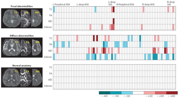
Examples of image-matrix conversions. The multiple raw MR images (e.g., T2, FA, MD) are parcellated into approximately 200 structures, from which their size, T2, FA, and MD values are then quantified. This converts the three MR images into a 4 × 200 standardized matrix. If we have the same matrices from age-matched control subjects, the amount of deviation from the normal average (z-score) can be calculated. Examples include patient brains with focal and diffuse abnormalities and controls. These standardized and quantitative matrices are directly comparable across subjects and are searchable in the database. Abbreviations: FA, fractional anisotrophy; GM, gray matter; L, left; MD, mean diffusivity; R, right; SD, standard deviation; WM, white matter.

3.4. Data Retrieval from a Neuroinformatics Database

If the text fields for clinical information are structured, physicians can search, for example, on the phrase “past cases with a diagnosis of Alzheimer’s disease,” which might return 100 images of AD patients. Although the retrieved images would be very useful for research purposes, they would not be useful for everyday clinical decisions. The searching strategy for clinical neuroinformatics is fundamentally different because a direct search of images is possible: Physicians submit an image of a new patient and search 100 past cases with similar anatomical phenotypes. The clinical reports of the 100 patients are then retrieved, and a statistical report of the diagnosis (e.g., 80% AD) and prognosis (e.g., time course of memory performance) is generated. The technology for direct image search is called content-based image retrieval (CBIR) and is similar to face recognition programs (for review, see 47). This technology has been tested for CT (48–50) and MRI (51–55) but, to date, has seldom been used in routine clinical practice or in educational resources (47). Two difficulties in applying CBIR to the human brain are the complexity of the structures and the importance of location information. Quantitative and standardized structural identification by image-matrix conversion is expected to allow images to be structured, thereby making a direct image search possible. This is the key to unlocking the vast amount of information currently stored in a PACS and using that information to make modern, evidence-based medical decisions.

3.5. Evaluation of Anatomical Phenotypes Stored in Anatomical Matrices

To simplify, consider an anatomical matrix with only one row, the volumes. This means that a 15-MB T1-weighted image is converted to a 200-element vector; each element contains the volume of a structure, and the elements collectively represent the brain shape. These volumes are a 200-dimensional representation of the anatomical phenotype. If we were interested in, for example, the neurological diseases of aging populations, it would be feasible to collect 10,000 past cases from a clinical database, which would include various types of geriatric conditions, such as ischemic lesions, frontal atrophy, and various anatomical changes caused by neurodegenerative diseases. If all these images were converted to 200-element vectors and the database also contained clinical information, we would have a neuroinformatics database of brain anatomical phenotypes, in which the image information would be structured. When examining the anatomical phenotype of a new patient, we would compare his or her anatomical matrix with the existing matrices in the database. In neuroinformatics, we are far more interested in the anatomical relationship with past patients who share similar anatomical phenotypes, rather thanin group comparisons with aggregated statistical reports, such as averages and standard deviations of each element of the anatomical matrices.

To evaluate the features of anatomical phenotypes, we can simply plot the 10,000 data points in the 200-dimensional space, which is called an anatomical landscape. Just like two values, latitude and longitude, can define a location on the earth, 200 values can define the anatomical position of a patient within the anatomical landscape. This location corresponds to anatomical information about diagnosis, prognosis, and other clinically meaningful outcomes. Interestingly, it becomes clear, as soon as this type of relational analysis is undertaken, that 200 is still a large number to evaluate easily. First, all 200 numbers are not independent. For example, the atrophy of the hippocampus is usually linked to an increased size of the inferior horn of the lateral ventricle. Therefore, two independent measures of these two structures would provide redundant information. Second, too many measured parameters with noise and redundancy can weaken the soundness of subsequent anatomy-function correlation analyses. Thus, further reduction of the granularity scale is required to represent the anatomy (Figure 1).

To evaluate the amount of information in the anatomical matrix, principal component analysis (PCA) can be performed, reducing the 200-dimensional information into a smaller number of principal components. Each principal component in the PCA represents a linear combination of the original 200 elements. In the above example, the volumes of the hippocampus and the inferior horn of the lateral ventricle should be combined into a single axis. Figure 5 shows an example of PCA, in which only the first three principal components are shown for visualization purposes. In this analysis, patients with primary progressive aphasia (PPA), a neurodegenerative clinical syndrome that causes progressive decline in language, and age-matched control subjects are plotted. These three principal axes explain 50.3% of anatomical variations in these populations. The diagnosis was based on clinical signs, not anatomical phenotypes. The anatomical phenotypes were based on the 200-element anatomical matrix, which was automatically generated from T1-weighted images, without prior knowledge of the diagnosis. The segregation of the two groups in Figure 5 is thus naturally achieved. As informative as Figure 5 is, the accuracy of the segregation is not adequate to reach a diagnosis because there is significant overlap among the two populations. If the final purpose of the quantitative analysis were to achieve a clinical diagnosis, this approach would fail. However, neuroinformatics for clinical diagnosis is not intended to replace human judgment; instead, it is meant to provide a structured past medical record and support more systematic evidence-based image reading. Radiological decisions are currently based solely on a radiologist’s expert opinion, which is ranked as the lowest level of evidence (LOE) in modern evidence-based medicine (56). Neuroinformatics for clinical diagnosis aims to increase the image reading’s LOE by providing a platform with which to quantitatively describe image features.

Figure 5.

Principal component analysis (PCA) of anatomical matrices of primary progressive aphasia (PPA) patients and age-matched controls. The first three principal component (PC) axes account for 50.3% of observed variability in the anatomical matrices. Although the two groups are segregated in this space, there is a substantial amount of overlap. This could be due to a failure of the anatomical matrices to capture clinically important anatomical features. However, close inspection of outliers, such as the case indicated by a green arrow, reveals that their anatomy is, indeed, a typical of patients with the clinical phenotype of PPA. In this way, anatomical and clinical phenotypes of individuals can be systematically compared with population data.

For example, there could be a PPA patient whose anatomical phenotype is localized within the control subjects (indicated by an arrow in Figure 5). An anatomical evaluation of this patient indicated normal-appearing anatomy; two radiologists blinded to the diagnosis described the patient’s anatomy as normal, yet the patient’s symptoms fulfill the diagnostic criteria of PPA. Thus, the 200-element anatomical matrix could not separate this patient from controls not because the matrix was unable to capture apparent brain atrophy but because the patient’s anatomy was indeed a typical of a patient with clinical symptoms of PPA. Such a patient’s pathological state must certainly be closely monitored. For example, were there any past records with similar anatomical and clinical phenotypes? If so, what were the prognoses for those patients, and what were their final diagnoses? These questions could be easily answered by searching past cases, based on the anatomical matrices, and comparing the prognoses of patients with typical and a typical anatomical features or seeking a correlation between how typical the image is and how good or poor the prognosis was. Although this is retrospective research, the LOE would already be higher than that of expert opinions alone. This type of systematic management of past anatomical and clinical descriptions of individual patients will afford a new opportunity to deepen our understanding about patients’ clinical states, prognoses, and intervention options. Neuroinformatics may also help to create a higher LOE by introducing objective inclusion or exclusion criteria for prospective cohort studies.

3.6. Extension to Machine Learning by Integrating Anatomical and Clinical Phenotypes

PCA is based purely on the anatomical matrix, in which all 200 structures have equal significance. However, when physicians evaluate MR images, they implicitly place weights on several key structures that are related to specific diseases. In Huntington’s disease, for example, the caudate and putamen are known to be two of the earliest-affected structures; in AD, temporal lobe atrophy is apparent early, often signaled via hippocampal change. Doctors learn the relationships between a specific disease and anatomical phenotypes; such knowledge is not always reproducible or specific, but it may provide an important clue about a patient’s pathological state. To achieve similar connections using an MRI brain database, machine-learning approaches, such as linear discriminant analysis (LDA) or support vector machines (57–59), can be used to index the anatomical data with diagnostic labelings from the groups; for example, in Figure 5, we entered information about clinical labels (clinically normal for PPA) and calculated the anatomical features that were associated with a specific disease. In Figure 6, the results of discriminant analysis are shown, and PPA patients are differentiated from controls with high sensitivity and specificity. Although these results seem to support LDA’s use as an automated diagnosis tool, care must be taken. Because of the high number of measured parameters (200), it is highly likely that, simply by chance, this method could identify a combination of structural volumes that could separate two groups with high accuracy. The true sensitivity and specificity must be tested using a great deal of data. Nonetheless, if there were many existing data in a neuroinformatics database, population-based analysis such as LDA could analyze the anatomical phenotypes of patients and provide probabilistic information about the diagnosis based on past cases, which could, in turn, enrich physicians’ decision-making processes.

Figure 6.

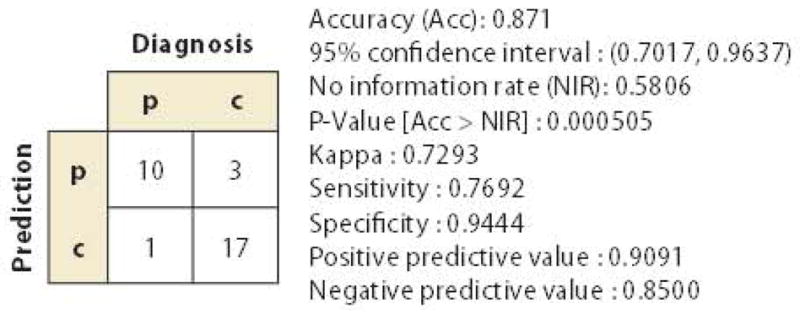
A result of partial least squares discriminant analysis based on the results shown in Figure 4. In this analysis, the anatomical features in the anatomical matrices that maximize the separation of the two groups [patients (p) and controls (c)] are extracted from a training data set (n = 38) and tested for the ability to diagnose PPA in a test data set (n = 31). It is important to note that the purpose of this analysis was not to test the accuracy of automated diagnosis based on population data but rather to provide information about individual pathology status by incorporating both anatomical and clinical information. Specifically, if a new PPA patient is categorized in the p (diagnosis)/p (anatomy-based prediction) class, this patient has typical PPA-type anatomical features. If, however, a patient is diagnosed with PPA based on clinical symptoms but does not have PPA-like anatomical features (p/c class), the physician should be aware of the potential for misdiagnosis or for a special subtype of PPA with a different time course or outcome.

3.7. Issues Related to Automated Parcellation Technologies

In sections above, we described strategies to analyze the anatomical information captured by anatomical matrices. However, there remain questions about anatomical matrices themselves, namely, the accuracy of the brain parcellation and the representativeness of the anatomical phenotypes (i.e., whether the anatomical matrices effectively represent important anatomical features). As shown in Figure 2, there are multiple criteria by which to parcellate a brain, and it is the operator, not an algorithm, who defines the criteria of interest. Usually, the criteria are entered into an automated parcellation algorithm in the form of a preparcellated atlas (Figures 2 and 3). The boundaries of defined structures are based on anatomical contrasts (e.g., gray matter versus white matter) or anatomical landmarks (e.g., the anterior limb of the internal capsule is the white matter between the caudate and the lenticular nuclei). Structures that are not visible by MRI, because of lack of either contrast or spatial resolution, cannot be reliably parcellated, which limits the definable structures. For example, the dentate nuclei of the hippocampus can be defined in an atlas, but the automated parcellation results are not reliable because they cannot be seen on conventional MR images.

The level of granularity (Figure 1) is a very important factor when considering parcellation accuracy and representativeness. Theoretically, the smallest granularity is defined by the voxel size. This minimum unit is defined by SNR and is, therefore, hardware driven. Parcellation is achieved by clustering voxels based on criteria defined by the atlas of choice. As mentioned above, parcellation is reliable if the target structures have clear contrasts and/or anatomical landmarks. In this sense, the parcellation criteria are image driven. The atlas shown in Figure 3a contains about 200 structures that can be clearly defined by T1, T2, and DTI contrasts. This 200-dimensional representation is a near 10,000-fold reduction in data and, as discussed above, must therefore be designed so as not to obliterate the highly localized abnormalities through the voxel grouping. The minimum granularity (one voxel) is hardware driven, and the parcellated structures are image driven. Still missing from this discussion are the clinically-driven demands; in other words, What granularity level is needed to support clinical practice? It is not a simple question because the required level of granularity changes dynamically, depending on the potential diseases in a physician’s knowledge and experience. Sometimes physicians look for lobar-level atrophy patterns (e.g., Is atrophy global or focused in the left temporal lobes?) or at a specific structure (e.g., Does rostral midbrain atrophy exist in this patient with a typical Parkinsonism?). In an interesting recent test, we parcellated the brains of five elderly patients and asked two radiologists and one neurologist to examine each of the 200 parcels and judge whether there was atrophy using a three-point scale [0 (normal), 1 (apparent atrophy), and 2 (severe atrophy)]. The agreement among the three physicians was rather low (r = 0.58). However, when some of the 200 parcels were combined to create an atlas with lower granularity (14 parcels), the agreement improved significantly (r = 0.84). This test indicates that the level of granularity for visual examination is, in general, lower than 200. Of course, anatomical granularity is not a simple concept because, as described above, physicians have very flexible views about it, and the incorporation of such flexibility in an atlas is one of the greatest challenges for creating image-based analysis appropriate for the clinical environment.

With these issues in mind, we must make the following assumptions: (a) Measurements of anatomical properties based on classical structural definitions can effectively represent anatomical phenotypes that are clinically important, and (b) daily radiological reading is based on anatomical phenotypes that are clearly visible on conventional MRI and can be represented with a granularity level of about 200 or less. The remaining issue is the ability to accurately define the structures.

Roughly speaking, there are two types of solutions for achieving automated brain parcellation. The first category is based on local solutions (60–69). Typically, the target of this approach is the parcellation of a single structure or multiple structures (e.g., hippocampus parcellation). This approach often requires probabilistic prior information about the location of the structure(s) of interest. The second category is based on a global solution (70–75), an approach that shares the same procedure as VBA—the mapping of all the voxels in one brain to all the voxels in another brain. When the voxel-to-voxel mapping is completed, the structural definition file (Figure 2) can be readily transferred from one brain to the other, achieving the parcellation of targeted structures or the entire brain at once (Figure 3) (13, 76–85). As the local approach extends to a larger number of target structures, the distinction between the two approaches diminishes.

Atlases defined by a single subject are the simplest form of atlas [e.g., the Talairach atlas (39), Colin 27 atlas (29), or the Eve white matter atlas (86)], but these atlases have been criticized because they do not represent population-averaged anatomy. The existence of subject-specific anatomical features can hurt the accuracy of voxel-to-voxel mapping and subsequent quantification. Obviously, the more similar the anatomies of the two brains, the more accurate the image transformation (voxel-to-voxel mapping) is. To expand the anatomical range of the operation of a single-subject atlas, the transformation method can be improved. For example, diffeomorphic transformation is designed to achieve greater accuracy even when the shape difference of two objects is large (77, 87–89). However, there is always a limit to the anatomical range of applicability. A single-subject atlas can serve as the origin of the coordinates from which the anatomies of many subjects is measured. If the atlas is derived from a young adult, it may not be optimum to investigate geriatric or pediatric populations using that atlas. To accommodate age-dependent anatomical changes, the concept of age-matched atlases has emerged (Figure 2f). Population-averaged atlases are expected to have a brain shape that represents the population of interest and provides better mapping accuracy (9, 90–93). A population-averaged atlas is typically created by iterative averaging (linear addition of images) of the populations of interest. One drawback of this approach is that the population representativeness is a moving target; as a result, to maximize the expected accuracy, an atlas must be created for each population at a given age range.

The heterogeneity of the anatomical phenotypes observed in clinical practice (Table 1) is troublesome for both single-subject and population-averaged atlases because the expected range of anatomical variability is large and unpredictable. The notion of population-representative anatomy is not very meaningful if the location and nature of anatomical phenotypes are incoherent. Similar to the age-matched atlas selections described above (Figure 2f), multiatlas brain mapping has recently emerged (73, 84, 94–103). Rather than generating a single population-averaged atlas by averaging, for example, 100 brain images with heterogeneous anatomies, we keep the original 100 unaveraged images and perform 100 brain mappings to a patient image. This is obviously a much more computationally extensive approach. Among the 100 atlases, some atlases would be anatomically closer to the patient than other atlases would be. The parcellation results from these 100 atlases could be combined either with equal weighting or with weighting based on various types of information, such as global or local anatomical similarity between the atlas and the patient. The multiatlas approach has the potential to accommodate the large anatomical variability encountered in clinical cases and to deliver a high level of parcellation accuracy.

4. FUTURE EXTENSION OF MULTIATLAS-BASED PARCELLATION WITHIN THE CONTEXT OF A NEUROINFORMATICS DATABASE

A multiatlas approach requires an array of fully parcellated atlases. For clinical applications, the inventory of these preparcellated atlases must necessarily cover the wide range of anatomical variability that would be encountered in clinical practice. One interesting extension of the clinical neuroinformatics database is to use past clinical cases for a multiatlas approach. In sections above, the structured data in the database were treated as targets of image search and retrieval, but for the multiatlas analyses, the anatomical labels are actively used to improve the parcellation of new patient data. An appropriate set of structured data could be selected based on anatomical similarity measured by, for example, distances between the target image and atlases in the dimension-reduced PCA/LDA space. The initial anatomical matrices could be derived from a single-atlas approach as a rough estimation of the patient anatomy, followed by more accurate multiatlas parcellation using existing patient data, from the database, that share similar anatomical phenotypes.

The purpose of the multiatlas approach is to use the multiple anatomical templates to achieve accurate brain parcellation, regardless of anatomical variability. However, for clinical neuroinformatics, the final goal is not accurate parcellation per se; rather, we want to obtain clinically meaningful information (e.g., diagnosis or prognosis). The process of defining appropriate atlases and achieving accurate parcellation can be considered an attempt to define the precise location of the patient within the anatomical landscape; the parcellation is thus a means by which to identify the precise location. In this sense, the image search and multiatlas structural characterization will evolve as an interactive and integrated tool for clinical neuroinformatics in the future.

5. CONCLUSION

In this review, we have detailed the future roles of neuroinformatics in clinical diagnoses. Radiologists acquire the ability to read images through education and training and then correlate anatomical phenotypes with potential pathology. Current medical record systems, such as PACS, contain a wealth of information that could potentially replicate a clinician’s knowledge, but the contents of such medical record systems have not been readily available to enrich routine diagnostic practices. One of the substantial bottlenecks for the systematic utilization of the vast amount of existing imaging information is the structurization of anatomical phenotypes. Atlas-based image parcellation, which can systematically reduce the anatomical contents to quantitative and standardized matrices, has great potential as a tool for image structurization. We have also reported several concepts to utilize the standardized image information for an image-based database search and for characterization of anatomical phenotypes of an individual, with respect to patient population data. Of course, anatomical phenotypes are valuable only when they are organically related to text-based clinical information. The usefulness of clinical neuroinformatics will therefore rely on the development of both image-based and text-based informatics from medical records, which development will mandate interdisciplinary efforts in the future.

LITERATURE CITED

- 1.Ashburner J, Friston KJ. Nonlinear spatial normalization using basis functions. Hum Brain Mapp. 1999;7:254–66. doi: 10.1002/(SICI)1097-0193(1999)7:4<254::AID-HBM4>3.0.CO;2-G. [DOI] [PMC free article] [PubMed] [Google Scholar]
- 2.Good CD, Johnsrude IS, Ashburner J, Henson RN, Friston KJ, Frackowiak RS. A voxel-based morphometric study of ageing in 465 normal adult human brains. NeuroImage. 2001;14:21–36. doi: 10.1006/nimg.2001.0786. [DOI] [PubMed] [Google Scholar]
- 3.Smith SM, Jenkinson M, Johansen-Berg H, Rueckert D, Nichols TE, et al. Tract-based spatial statistics: voxelwise analysis of multi-subject diffusion data. NeuroImage. 2006;31:1487–505. doi: 10.1016/j.neuroimage.2006.02.024. [DOI] [PubMed] [Google Scholar]
- 4.Zhang H, Yushkevich PA, Alexander DC, Gee JC. Deformable registration of diffusion tensor MR images with explicit orientation optimization. Med Image Anal. 2006;10:764–85. doi: 10.1016/j.media.2006.06.004. [DOI] [PubMed] [Google Scholar]
- 5.Verma R, Mori S, Shen D, Yarowsky P, Zhang J, Davatzikos C. Spatiotemporal maturation patterns of murine brain quantified by diffusion tensor MRI and deformation-based morphometry. Proc Natl Acad Sci USA. 2005;102:6978–83. doi: 10.1073/pnas.0407828102. [DOI] [PMC free article] [PubMed] [Google Scholar]
- 6.Chiang MC, Leow AD, Klunder AD, Dutton RA, Barysheva M, et al. Fluid registration of diffusion tensor images using information theory. IEEE Trans Med Imaging. 2008;27:442–56. doi: 10.1109/TMI.2007.907326. [DOI] [PMC free article] [PubMed] [Google Scholar]
- 7.Yushkevich PA, Zhang H, Simon TJ, Gee JC. Structure-specific statistical mapping of white matter tracts. NeuroImage. 2008;41:448–61. doi: 10.1016/j.neuroimage.2008.01.013. [DOI] [PMC free article] [PubMed] [Google Scholar]
- 8.Wright IC, McGuire PK, Poline JB, Travere JM, Murray RM, et al. A voxel-based method for the statistical analysis of gray and white matter density applied to schizophrenia. NeuroImage. 1995;2:244–52. doi: 10.1006/nimg.1995.1032. [DOI] [PubMed] [Google Scholar]
- 9.Mazziotta J, Toga A, Evans A, Fox P, Lancaster J, et al. A probabilistic atlas and reference system for the human brain: International Consortium for Brain Mapping (ICBM) Philos Trans R Soc Lond B Biol Sci. 2001;356:1293–322. doi: 10.1098/rstb.2001.0915. [DOI] [PMC free article] [PubMed] [Google Scholar]
- 10.Ashburner J. Computational anatomy with the SPM software. Magn Reson Imaging. 2009;27:1163–74. doi: 10.1016/j.mri.2009.01.006. [DOI] [PubMed] [Google Scholar]
- 11.Smith SM, Jenkinson M, Woolrich MW, Beckmann CF, Behrens TE, et al. Advances in functional and structural MR image analysis and implementation as FSL. NeuroImage. 2004;23 (Suppl 1):S208–19. doi: 10.1016/j.neuroimage.2004.07.051. [DOI] [PubMed] [Google Scholar]
- 12.Rex DE, Ma JQ, Toga AW. The LONI Pipeline Processing Environment. NeuroImage. 2003;19:1033–48. doi: 10.1016/s1053-8119(03)00185-x. [DOI] [PubMed] [Google Scholar]
- 13.Collins DL, Holmes CJ, Peters TM, Evans AC. Automatic 3-D model-based neuroanatomical segmentation. Hum Brain Mapp. 1995;3:190–208. [Google Scholar]
- 14.US Gov. Account. Off. Medicare part B imaging services. Washington, DC: 2008. GAO-08-452. [Google Scholar]
- 15.Karimaghaloo Z, Shah M, Francis SJ, Arnold DL, Collins DL, Arbel T. Automatic detection of gadolinium-enhancing multiple sclerosis lesions in brain MRI using conditional random fields. IEEE Trans Med Imaging. 2012;31:1181–94. doi: 10.1109/TMI.2012.2186639. [DOI] [PubMed] [Google Scholar]
- 16.Elliott C, Francis SJ, Arnold DL, Collins DL, Arbel T. Bayesian classification of multiple sclerosis lesions in longitudinal MRI using subtraction images. Proc MICCAI LNCS. 2010;6362:290–97. doi: 10.1007/978-3-642-15745-5_36. [DOI] [PubMed] [Google Scholar]
- 17.Alfano B, Brunetti A, Larobina M, Quarantelli M, Tedeschi E, et al. Automated segmentation and measurement of global white matter lesion volume in patients with multiple sclerosis. J Magn Reson Imaging. 2000;12:799–807. doi: 10.1002/1522-2586(200012)12:6<799::aid-jmri2>3.0.co;2-#. [DOI] [PubMed] [Google Scholar]
- 18.Miki Y, Grossman RI, Udupa JK, Samarasekera S, van Buchem MA, et al. Computer-assisted quantitation of enhancing lesions in multiple sclerosis: correlation with clinical classification. AJNR Am J Neuroradiol. 1997;18:705–10. [PMC free article] [PubMed] [Google Scholar]
- 19.Bedell BJ, Narayana PA. Automatic segmentation of gadolinium-enhanced multiple sclerosis lesions. Magn Reson Med. 1998;39:935–40. doi: 10.1002/mrm.1910390611. [DOI] [PubMed] [Google Scholar]
- 20.Miller M, Banerjee A, Christensen G, Joshi S, Khaneja N, et al. Statistical methods in computational anatomy. Stat Methods Med Res. 1997;6:267–99. doi: 10.1177/096228029700600305. [DOI] [PubMed] [Google Scholar]
- 21.Toga AW, Thompson PM, Holmes CJ, Payne BA. Informatics and computational neuroanatomy. Proc. Am. Med. Inform. Assoc. (AMIA) Fall Symposium, Section S75; Washington, DC. Oct. 26–30; Bethesda, MD: AMIA; 1996. pp. 299–303. [PMC free article] [PubMed] [Google Scholar]
- 22.Mazziotta JC, Toga AW, Evans A, Fox P, Lancaster J. A probabilistic atlas of the human brain: theory and rationale for its development: the International Consortium for Brain Mapping (ICBM) NeuroImage. 1995;2:89–101. doi: 10.1006/nimg.1995.1012. [DOI] [PubMed] [Google Scholar]
- 23.Toga AW, editor. Visualization and Warping of Multi-modality Brain Imagery Functional Neuroimaging: Technical Foundations. San Diego: Academic; 1994. [Google Scholar]
- 24.Ashburner J, Friston KJ. Voxel-based morphometry—the methods. NeuroImage. 2000;11:805–21. doi: 10.1006/nimg.2000.0582. [DOI] [PubMed] [Google Scholar]
- 25.Bookstein FL. Landmark methods for forms without landmarks: morphometrics of group differences in outline shape. Med Image Anal. 1997;1:225–43. doi: 10.1016/s1361-8415(97)85012-8. [DOI] [PubMed] [Google Scholar]
- 26.Gee JC, Reivich M, Bajcsy R. Elastically deforming 3D atlas to match anatomical brain images. J Comput Assist Tomogr. 1993;17:225–36. doi: 10.1097/00004728-199303000-00011. [DOI] [PubMed] [Google Scholar]
- 27.Thompson PM, MacDonald D, Mega MS, Holmes CJ, Evans AC, Toga AW. Detection and mapping of abnormal brain structure with a probabilistic atlas of cortical surfaces. J Comput Assist Tomogr. 1997;21:567–81. doi: 10.1097/00004728-199707000-00008. [DOI] [PubMed] [Google Scholar]
- 28.Evans AC, Collins DL, Milner B. An MRI-based stereotactic atlas from 250 young normal subjects. Soc Neurosci Abstr. 1992;18:408–92. [Google Scholar]
- 29.Holmes CJ, Hoge R, Collins L, Woods R, Toga AW, Evans AC. Enhancement of MR images using registration for signal averaging. J Comput Assist Tomogr. 1998;22:324–33. doi: 10.1097/00004728-199803000-00032. [DOI] [PubMed] [Google Scholar]
- 30.Fonov V, Evans AC, Botteron K, Almli CR, McKinstry RC, Collins DL. Unbiased average age-appropriate atlases for pediatric studies. NeuroImage. 2011;54:313–27. doi: 10.1016/j.neuroimage.2010.07.033. [DOI] [PMC free article] [PubMed] [Google Scholar]
- 31.Mori S, Wakana S, Nagae-Poetscher LM, van Zijl PC. MRI Atlas of Human White Matter. Amsterdam, The Netherlands: Elsevier; 2005. [Google Scholar]
- 32.Wakana S, Jiang H, Nagae-Poetscher LM, Van Zijl PC, Mori S. Fiber tract-based atlas of human white matter anatomy. Radiology. 2004;230:77–87. doi: 10.1148/radiol.2301021640. [DOI] [PubMed] [Google Scholar]
- 33.Catani M, Thiebaut de Schotten M. A diffusion tensor imaging tractography atlas for virtual in vivo dissections. Cortex. 2008;44:1105–32. doi: 10.1016/j.cortex.2008.05.004. [DOI] [PubMed] [Google Scholar]
- 34.Toga AW, Thompson PM, Mori S, Amunts K, Zilles K. Towards multimodal atlases of the human brain. Nat Rev Neurosci. 2006;7:952–66. doi: 10.1038/nrn2012. [DOI] [PMC free article] [PubMed] [Google Scholar]
- 35.Drury HA, Van Essen DC, Anderson CH, Lee CW, Coogan TA, Lewis JW. Computerized mappings of the cerebral cortex: a multiresolution flattening method and a surface-based coordinate system. J Cogn Neurosci. 1996;8:1–28. doi: 10.1162/jocn.1996.8.1.1. [DOI] [PubMed] [Google Scholar]
- 36.Dale AM, Fischl B, Sereno MI. Cortical surface-based analysis. I Segmentation and surface re-construction. NeuroImage. 1999;9:179–94. doi: 10.1006/nimg.1998.0395. [DOI] [PubMed] [Google Scholar]
- 37.Fischl B, Sereno MI, Dale AM. Cortical surface-based analysis. II: Inflation, flattening, and a surface-based coordinate system. NeuroImage. 1999;9:195–207. doi: 10.1006/nimg.1998.0396. [DOI] [PubMed] [Google Scholar]
- 38.Chakravarty MM, Sadikot AF, Mongia S, Bertrand G, Collins DL. Towards a multi-modal atlas for neurosurgical planning. Proc MICCAI LCNS. 2006;4191:389–96. doi: 10.1007/11866763_48. [DOI] [PubMed] [Google Scholar]
- 39.Talairach J, Tournoux P. 3-Dimensional Proportional System: An Approach to Cerebral Imaging. New York: Thieme Medical; 1988. Co-planar Stereotaxic Atlas of the Human Brain. [Google Scholar]
- 40.Collins DL, Neelin P, Peters TM, Evans AC. Automatic 3D intersubject registration of MR volumetric data in standardized Talairach space. J Comput Assist Tomogr. 1994;18:192–205. [PubMed] [Google Scholar]
- 41.Ascoli GA, De Schutter E, Kennedy DN. An information science infrastructure for neuroscience. Neuroinformatics. 2003;1:1–2. doi: 10.1385/NI:1:1:001. [DOI] [PubMed] [Google Scholar]
- 42.Shepherd GM, Mirsky JS, Healy MD, Singer MS, Skoufos E, et al. The Human Brain Project: neuroinformatics tools for integrating, searching and modeling multidisciplinary neuroscience data. Trends Neurosci. 1998;21:460–68. doi: 10.1016/s0166-2236(98)01300-9. [DOI] [PubMed] [Google Scholar]
- 43.Langlotz CP. Structured radiology reporting: Are we there yet? Radiology. 2009;253:23–25. doi: 10.1148/radiol.2531091088. [DOI] [PubMed] [Google Scholar]
- 44.Kahn CE, Jr, Langlotz CP, Burnside ES, Carrino JA, Channin DS, et al. Toward best practices in radiology reporting. Radiology. 2009;252:852–56. doi: 10.1148/radiol.2523081992. [DOI] [PubMed] [Google Scholar]
- 45.Johnson AJ, Chen MY, Zapadka ME, Lyders EM, Littenberg B. Radiology report clarity: a cohort study of structured reporting compared with conventional dictation. JACR J Am Coll Radiol. 2010;7:501–6. doi: 10.1016/j.jacr.2010.02.008. [DOI] [PubMed] [Google Scholar]
- 46.Wong ST, Hoo KS, Jr, Cao X, Tjandra D, Fu JC, Dillon WP. A neuroinformatics database system for disease-oriented neuroimaging research. Acad Radiol. 2004;11:345–58. doi: 10.1016/s1076-6332(03)00676-7. [DOI] [PubMed] [Google Scholar]
- 47.Muller H, Michoux N, Bandon D, Geissbuhler A. A review of content-based image retrieval systems in medical applications—clinical benefits and future directions. Int J Med Inform. 2004;73:1–23. doi: 10.1016/j.ijmedinf.2003.11.024. [DOI] [PubMed] [Google Scholar]
- 48.Robinson GP, Tagare HD, Duncan JS, Jaffe CC. Medical image collection indexing: shape-based retrieval using KD-trees. Comput Med Imaging Graph. 1996;20:209–17. doi: 10.1016/s0895-6111(96)00014-6. [DOI] [PubMed] [Google Scholar]
- 49.Greenspan H, Pinhas AT. Medical image categorization and retrieval for PACS using the GMM-KL framework. IEEE Trans Inf Technol Biomed. 2007;11:190–202. doi: 10.1109/titb.2006.874191. [DOI] [PubMed] [Google Scholar]
- 50.Rahman MM, Bhattacharya P, Desai BC. A framework for medical image retrieval using machine learning and statistical similarity matching techniques with relevance feedback. IEEE Trans Inf Technol Biomed. 2007;11:58–69. doi: 10.1109/titb.2006.884364. [DOI] [PubMed] [Google Scholar]
- 51.El-Kwae EA, Xu H, Kabuka MR. Content-based retrieval in picture a rchiving and communication systems. J Digit Imaging. 2000;13:70–81. doi: 10.1007/BF03168371. [DOI] [PMC free article] [PubMed] [Google Scholar]
- 52.Orphanouda kis SC, Chronaki CE, Vamvaka D. I2Cnet Content-based similarity search in geographically distributed repositories of medical images. Comput Med Imaging Graph. 1996;20:193–207. doi: 10.1016/s0895-6111(96)00013-4. [DOI] [PubMed] [Google Scholar]
- 53.Sinha U, Ton A, Yaghmai A, Taira RK, Kangarloo H. Image content extraction: application to MR images of the brain. Radiographics. 2001;21:535–47. doi: 10.1148/radiographics.21.2.g01mr18535. [DOI] [PubMed] [Google Scholar]
- 54.Unay D, Ekin A, Jasinschi RS. Local structure-based region-of-interest retrieval in brain MR images. IEEE Trans Inf Technol Biomed. 2010;14:897–903. doi: 10.1109/TITB.2009.2038152. [DOI] [PubMed] [Google Scholar]
- 55.Muller H, Rosset A, Garcia A, Vallee JP, Geissbuhler A. Informatics in radiology (infoRAD): benefits of content-based visual data access in radiology. Radiographics. 2005;25:849–58. doi: 10.1148/rg.253045071. [DOI] [PubMed] [Google Scholar]
- 56.Hadorn DC, Baker D, Hodges JS, Hicks N. Rating the quality of evidence for clinical practice guidelines. J Clin Epidemiol. 1996;40:749–54. doi: 10.1016/0895-4356(96)00019-4. [DOI] [PubMed] [Google Scholar]
- 57.Wang S, Summers RM. Machine learning and radiology. Med Image Anal. 2012;16:933–51. doi: 10.1016/j.media.2012.02.005. [DOI] [PMC free article] [PubMed] [Google Scholar]
- 58.Mwangi B, Ebmeier KP, Matthews K, Steele JD. Multi-centre diagnostic classification of individual structural neuroimaging scans from patients with major depressive disorder. Brain: J Neurol. 2012;135:1508–21. doi: 10.1093/brain/aws084. [DOI] [PubMed] [Google Scholar]
- 59.Depeursinge A, Fischer B, Muller H, Deserno TM. Prototypes for content-based image retrieval in clinical practice. Open Med Inform J. 2011;5:58–72. doi: 10.2174/1874431101105010058. [DOI] [PMC free article] [PubMed] [Google Scholar]
- 60.Hill A, Cootes TF, Taylor CJ, Lindley K. Medical image interpretation: a generic approach using deformable templates. Med Inform (London) 1994;19:47–59. doi: 10.3109/14639239409044720. [DOI] [PubMed] [Google Scholar]
- 61.Duta N, Sonka M. Segmentation and interpretation of MR brain images: an improved active shape model. IEEE Trans Med Imaging. 1998;17:1049–62. doi: 10.1109/42.746716. [DOI] [PubMed] [Google Scholar]
- 62.Pham DL, Prince JL. Adaptive fuzzy segmentation of magnetic resonance images. IEEE Trans Med Imaging. 1999;18:737–52. doi: 10.1109/42.802752. [DOI] [PubMed] [Google Scholar]
- 63.Shen D, Herskovits EH, Davatzikos C. An adaptive-focus statistical shape model for segmentation and shape modeling of 3-D brain structures. IEEE Trans Med Imaging. 2001;20:257–70. doi: 10.1109/42.921475. [DOI] [PubMed] [Google Scholar]
- 64.van Ginneken B, Frangi AF, Staal JJ, ter Haar Romeny BM, Viergever MA. Active shape model segmentation with optimal features. IEEE Trans Med Imaging. 2002;21:924–33. doi: 10.1109/TMI.2002.803121. [DOI] [PubMed] [Google Scholar]
- 65.Van Leemput K, Maes F, Vandermeulen D, Suetens P. A unifying framework for partial volume segmentation of brain MR images. IEEE Trans Med Imaging. 2003;22:105–19. doi: 10.1109/TMI.2002.806587. [DOI] [PubMed] [Google Scholar]
- 66.Priebe CE, Miller MI, Ratnanather JT. Segmenting magnetic resonance images via hierarchical mixture modelling. Comput Stat Data Anal. 2006;50:551–67. doi: 10.1016/j.csda.2004.09.003. [DOI] [PMC free article] [PubMed] [Google Scholar]
- 67.Awate SP, Zhang H, Gee JC. Fuzzy nonparametric DTI segmentation for robust cingulum-tract extraction. Proc MICCAI LCNS. 2007;4791:294–301. doi: 10.1007/978-3-540-75757-3_36. [DOI] [PubMed] [Google Scholar]
- 68.Tu Z, Narr KL, Dollar P, Dinov I, Thompson PM, Toga AW. Brain anatomical structure segmentation by hybrid discriminative/generative models. IEEE Trans Med Imaging. 2008;27:495–508. doi: 10.1109/TMI.2007.908121. [DOI] [PMC free article] [PubMed] [Google Scholar]
- 69.Patenaude B, Smith SM, Kennedy DN, Jenkinson M. A Bayesian model of shape and appearance for subcortical brain segmentation. NeuroImage. 2011;56:907–22. doi: 10.1016/j.neuroimage.2011.02.046. [DOI] [PMC free article] [PubMed] [Google Scholar]
- 70.Held K, Rota Kops E, Krause JB, Wells WM, III, Kikinis R, Müller-Gärtner HW. Markov random field segmentation of brain MR images. IEEE Trans Med Imaging. 1997;16:878–86. doi: 10.1109/42.650883. [DOI] [PubMed] [Google Scholar]
- 71.Baillard C, Hellier P, Barillot C. Segmentation of brain 3D MR images using level sets and dense registration. Med Image Anal. 2001;5:185–94. doi: 10.1016/s1361-8415(01)00039-1. [DOI] [PubMed] [Google Scholar]
- 72.Zhang Y, Brady M, Smith S. Segmentation of brain MR images through a hidden Markov random field model and the expectation-maximization algorithm. IEEE Trans Med Imaging. 2001;20:45–57. doi: 10.1109/42.906424. [DOI] [PubMed] [Google Scholar]
- 73.Fischl B, Salat DH, Busa E, Albert M, Dieterich M, et al. Whole brain segmentation: automated labeling of neuroanatomical structures in the human brain. Neuron. 2002;33:341–55. doi: 10.1016/s0896-6273(02)00569-x. [DOI] [PubMed] [Google Scholar]
- 74.Paragios N. A level set approach for shape-driven segmentation and tracking of the left ventricle. IEEE Trans Med Imaging. 2003;22:773–76. doi: 10.1109/TMI.2003.814785. [DOI] [PubMed] [Google Scholar]
- 75.Yang J, Duncan JS. 3D image segmentation of deformable objects with joint shape-intensity prior models using level sets. Med Image Anal. 2004;8:285–94. doi: 10.1016/j.media.2004.06.008. [DOI] [PMC free article] [PubMed] [Google Scholar]
- 76.Bajcsy R, Lieberson R, Reivich M. A computerized system for the elastic matching of deformed radiographic images to idealized atlas images. J Comput Assist Tomogr. 1983;7:618–25. doi: 10.1097/00004728-198308000-00008. [DOI] [PubMed] [Google Scholar]
- 77.Christensen GE, Joshi SC, Miller MI. Volumetric transformation of brain anatomy. IEEE Trans Med Imaging. 1997;16:864–77. doi: 10.1109/42.650882. [DOI] [PubMed] [Google Scholar]
- 78.Miller MI, Christensen GE, Amit Y, Grenander U. Mathematical textbook of deformable neuroanatomies. Proc Natl Acad Sci USA. 1993;90:11944–48. doi: 10.1073/pnas.90.24.11944. [DOI] [PMC free article] [PubMed] [Google Scholar]
- 79.Haller JW, Banerjee A, Christensen GE, Gado M, Joshi S, et al. Three-dimensional hippocampal MR morphometry with high-dimensional transformation of a neuroanatomic atlas. Radiology. 1997;202:504–10. doi: 10.1148/radiology.202.2.9015081. [DOI] [PubMed] [Google Scholar]
- 80.Warfield S, Robatino A, Dengler J, Jolesz F, Kikinis R. Nonlinear registration and template-driven segmentation. In: Toga A, editor. Brain Warping. San Diego: Academic; 1999. pp. 67–84. [Google Scholar]
- 81.Hogan RE, Mark KE, Wang L, Joshi S, Miller MI, Bucholz RD. Mesial temporal sclerosis and termporal lobe epilepsy: MR imaging deformation-based segmentation of the hippocampus in five patients. Radiology. 2000;216:291–97. doi: 10.1148/radiology.216.1.r00jl41291. [DOI] [PubMed] [Google Scholar]
- 82.Crum WR, Scahill RI, Fox NC. Automated hippocampal segmentation by regional fluid registration of serial MRI: validation and application in Alzheimer’s disease. NeuroImage. 2001;13:847–55. doi: 10.1006/nimg.2001.0744. [DOI] [PubMed] [Google Scholar]
- 83.Carmichael OT, Aizenstein HA, Davis SW, Becker JT, Thompson PM, et al. Atlas-based hippocampus segmentation in Alzheimer’s disease and mild cognitive impairment. NeuroImage. 2005;27:979–90. doi: 10.1016/j.neuroimage.2005.05.005. [DOI] [PMC free article] [PubMed] [Google Scholar]
- 84.Heckemann RA, Hajnal JV, Aljabar P, Rueckert D, Hammers A. Automatic anatomical brain MRI segmentation combining label propagation and decision fusion. NeuroImage. 2006;33:115–26. doi: 10.1016/j.neuroimage.2006.05.061. [DOI] [PubMed] [Google Scholar]
- 85.Pohl KM, Fisher J, Grimson WE, Kikinis R, Wells WM. A Bayesian model for joint segmentation and registration. NeuroImage. 2006;31:228–39. doi: 10.1016/j.neuroimage.2005.11.044. [DOI] [PubMed] [Google Scholar]
- 86.Oishi K, Faria A, Jiang H, Li X, Akhter K, et al. Atlas-based whole brain white matter analysis using large deformation diffeomorphic metric mapping: application to normal elderly and Alzheimer’s disease participants. NeuroImage. 2009;46:486–99. doi: 10.1016/j.neuroimage.2009.01.002. [DOI] [PMC free article] [PubMed] [Google Scholar]
- 87.Ashburner J. A fast diffeomorphic image registration algorithm. NeuroImage. 2007;38:95–113. doi: 10.1016/j.neuroimage.2007.07.007. [DOI] [PubMed] [Google Scholar]
- 88.Ceritoglu C, Oishi K, Li X, Chou MC, Younes L, et al. Multi-contrast large deformation diffeomorphic metric mapping for diffusion tensor imaging. NeuroImage. 2009;47:618–27. doi: 10.1016/j.neuroimage.2009.04.057. [DOI] [PMC free article] [PubMed] [Google Scholar]
- 89.Vercauteren T, Pennec X, Perchant A, Ayache N. Diffeomorphic demons: efficient non-parametric image registration. NeuroImage. 2009;45:S61–72. doi: 10.1016/j.neuroimage.2008.10.040. [DOI] [PubMed] [Google Scholar]
- 90.Evans AC, Collins DL, Mills SR, Brown ED, Kelly RL, Peters TM. 3D statistical neuroanatomical models from 305 MRI volumes. Nucl Sci. Symp. Med. Imaging Conf.; IEEE Conf. Record; Oct. 31-Nov. 6; 1993. pp. 1813–17. [Google Scholar]
- 91.Holmes CJ, Hoge R, Collins L, Woods R, Toga AW, Evans AC. Enhancement of MR images using registration for signal averaging. J Comput Assist Tomogr. 1998;22:324–33. doi: 10.1097/00004728-199803000-00032. [DOI] [PubMed] [Google Scholar]
- 92.Thompson PM, Woods RP, Mega MS, Toga AW. Mathematical/computational challenges in creating deformable and probabilistic atlases of the human brain. Hum Brain Mapp. 2000;9:81–92. doi: 10.1002/(SICI)1097-0193(200002)9:2<81::AID-HBM3>3.0.CO;2-8. [DOI] [PMC free article] [PubMed] [Google Scholar]
- 93.Evans AC, Janke AL, Collins DL, Baillet S. Brain templates and atlases. NeuroImage. 2012;62:911–22. doi: 10.1016/j.neuroimage.2012.01.024. [DOI] [PubMed] [Google Scholar]
- 94.Klein A, Hirsch J. Mindboggle: a scatterbrained approach to automate brain labeling. NeuroImage. 2005;24:261–80. doi: 10.1016/j.neuroimage.2004.09.016. [DOI] [PubMed] [Google Scholar]
- 95.Warfield SK, Zou KH, Wells WM. Simultaneous truth and performance level estimation (STAPLE): an algorithm for the validation of image segmentation. IEEE Trans Med Imaging. 2004;23:903–21. doi: 10.1109/TMI.2004.828354. [DOI] [PMC free article] [PubMed] [Google Scholar]
- 96.Rohlfing T, Brandt R, Menzel R, Maurer CR., Jr Evaluation of atlas selection strategies for atlas-based image segmentation with application to confocal microscopy images of bee brains. NeuroImage. 2004;21:1428–42. doi: 10.1016/j.neuroimage.2003.11.010. [DOI] [PubMed] [Google Scholar]
- 97.Aljabar P, Heckemann RA, Hammers A, Hajnal JV, Rueckert D. Multi-atlas based segmentation of brain images: atlas selection and its effect on accuracy. NeuroImage. 2009;46:726–38. doi: 10.1016/j.neuroimage.2009.02.018. [DOI] [PubMed] [Google Scholar]
- 98.Lotjonen JM, Wolz R, Koikkalainen JR, Thurfjell L, Waldernar G, et al. Fast and robust multi-atlas segmentation of brain magnetic resonance images. NeuroImage. 2010;49:2352–65. doi: 10.1016/j.neuroimage.2009.10.026. [DOI] [PubMed] [Google Scholar]
- 99.Wu M, Rosano C, Lopez-Garcia P, Carter CS, Aizenstein HJ. Optimum template selection for atlas-based segmentation. NeuroImage. 2007;34:1612–18. doi: 10.1016/j.neuroimage.2006.07.050. [DOI] [PubMed] [Google Scholar]
- 100.Yushkevich PA, Avants BB, Pluta J, Das S, Minkoff D, et al. A high-resolution computational atlas of the human hippocampus from postmortem magnetic resonance imaging at 9.4 T. NeuroImage. 2009;44:385–98. doi: 10.1016/j.neuroimage.2008.08.04. [DOI] [PMC free article] [PubMed] [Google Scholar]
- 101.Artaechevarria X, Munoz-Barrutia A, Ortiz-de-Solorzano C. Combination strategies in multi-atlas image segmentation: application to brain MR data. IEEE Trans Med Imaging. 2009;28:1266–77. doi: 10.1109/TMI.2009.2014372. [DOI] [PubMed] [Google Scholar]
- 102.Langerak TR, van der Heide UA, Kotte AN, Viergever MA, van Vulpen M, Pluim JP. Label fusion in atlas-based segmentation using a selective and iterative method for performance level estimation (SIMPLE) IEEE Trans Med Imaging. 2010;29:2000–8. doi: 10.1109/TMI.2010.2057442. [DOI] [PubMed] [Google Scholar]
- 103.van Rikxoort EM, Isgum I, Arzhaeva Y, Staring M, Klein S, et al. Adaptive local multi-atlas segmentation: application to the heart and the caudate nucleus. Med Image Anal. 2010;14:39–49. doi: 10.1016/j.media.2009.10.001. [DOI] [PubMed] [Google Scholar]
- 104.Faria AV, Zhang JY, Oishi K, Li X, Jiang HY, et al. Atlas-based analysis of neurodevelopment from infancy to adulthood using diffusion tensor imaging and applications for automated abnormality detection. NeuroImage. 2010;52:415–28. doi: 10.1016/j.neuroimage.2010.04.238. [DOI] [PMC free article] [PubMed] [Google Scholar]