

Abstract
An interaction energy decomposition analysis method based on the block-localized wavefunction (BLW-ED) approach is described. The first main feature of the BLW-ED method is that it combines concepts of valence bond and molecular orbital theories such that the intermediate and physically intuitive electron-localized states are variationally optimized by self-consistent field calculations. Furthermore, the block-localization scheme can be used both in wave function theory and in density functional theory, providing a useful tool to gain insights on intermolecular interactions that would otherwise be difficult to obtain using the delocalized Kohn–Sham DFT. These features allow broad applications of the BLW method to energy decomposition (BLW-ED) analysis for intermolecular interactions. In this perspective, we outline theoretical aspects of the BLW-ED method, and illustrate its applications in hydrogen-bonding and π–cation intermolecular interactions as well as metal–carbonyl complexes. Future prospects on the development of a multistate density functional theory (MSDFT) are presented, making use of block-localized electronic states as the basis configurations.
1. Introduction
Intermolecular interactions, particularly non-covalent interactions, play a key role in the formation of novel materials and folded structures of biological macromolecules. Of great interest is to use theoretical methods to decipher the individual energy components, which cannot be individually measured experimentally, and to elucidate the physical principles governing the overall intermolecular interactions. Although the specific definition of energy terms is far from stringent, energy decomposition analyses (EDA) can nevertheless help to provide a deeper understanding of intermolecular interactions, and to guide the development of force fields in computer simulations of nano-materials and biological systems,1 and in the rational design of inhibitors,2–5 and proteins with enhanced catalytic efficiency.6–9 In this perspective, we highlight an interaction energy decomposition analysis based on a block-localized wavefunction, called BLW-ED, and its extension to multistate density functional theory (MSDFT), along with selected applications.
A variety of interaction energy decomposition schemes have been proposed in the literature, most of which are based on a supermolecular model.10–21 Thus, if a supermolecular complex is composed of k monomers, the total binding energy (ΔEb) can be defined as the energy change from the infinitely separated monomers to the supermolecular complex:
| (1) |
where is the energy of monomer i, and ESuper is the total energy of the supermolecular complex, including counterpoise (CP) correction22 to account for the basis set superposition error (BSSE). The concept of interaction energy decomposition was developed on the basis of the Hartree–Fock (HF) theory by Morokuma, who partitioned the total interaction energy into electrostatic (ES), exchange repulsion (EX), polarization (PL), and charge transfer (CT) components.10 In the subsequent Morokuma–Kitaura approach, which is different from and should not be confused with the original Morokuma analysis,10 the energy components are derived from the change in the total energy when certain interaction matrix elements in the Fock and overlap matrices are zeroed. However, not all energy components are consistently defined,11e.g., the polarization energy does not satisfy the Pauli exclusion principle,23 resulting in a residual energy term to compensate for the fact that the sum of energy components is not exactly equal to the total interaction energy. To study intra-unit charge polarization and inter-unit electron donation in transition metal complexes, Bagus et al. proposed a constrained space orbital variations (CSOV) method which starts from the occupied and virtual molecular orbitals (MOs) of two subunits and successively allows the variation of the occupied MOs of one subunit into the virtual MOs of its own and the other unit.14 The CSOV has been generalized to open-shell cases24 and extended to density functional theory (DFT).25–27 Although the incorporation of electron correlation increases the charge transfer energy, the physical mechanisms from the CSOV analyses at both HF and DFT levels are essentially the same.25 Similarly, Stevens and Fink developed the reduced variational space self-consistent-field (RVS SCF) method where the MOs of one fragment are optimized in the field of the frozen orbitals of the other fragment.15 This approach is similar but not identical to the methods presented here. Another useful method is the natural energy decomposition analysis (NEDA),16 in which intermediate supermolecular and fragmental wave functions are constructed using natural bond orbitals.28,29 The NEDA method has also been extended to DFT.30 Focusing on the population instead of energetic variations in the interactions, notably Dapprich and Frenking developed a charge decomposition analysis in which the wave function of the complex is constructed in terms of a linear combination of the donor and acceptor fragment orbitals.31
Employing density functional theory, Ziegler and coworkers developed the extended transition state (ETS) scheme which divides the total interaction energy into electrostatic interaction, Pauli interaction, and orbital interaction energies.13,32,33 In contrast to other EDA approaches which deal with non-covalent (thus relatively weak) intermolecular interactions, the ETS energy decomposition method allows a chemical bond to be broken into fragments with unpaired electrons to explore chemical bonding interactions within a molecule.34–36 A further combination of the ETS method with the natural orbitals for chemical valence (NOCV) theory37 provided the capability of decomposing electron deformation density and bond energy into various components with chemical bonding characters such as σ, π, δ etc. bonds.38 In another variant, Wu et al.20 proposed a density-based EDA scheme using a constrained DFT formalism.39 Similarly, an EDA based on fragment-localized Kohn–Sham orbitals was developed by Reinhardt et al.19 Additional approaches focus on energy decomposition into contributions from molecular fragments or even atoms such as the molecular energy decomposition for atoms in a molecule.40–44
The second route to decomposing interaction energies is based on perturbation theory.45–48 One of the most popular schemes in this category is the symmetry-adapted perturbation theory (SAPT), which has been derived using both wave function theory and density functional theory.49–53 The SAPT method divides the total Hamiltonian into monomer Fock operators, monomer Møller–Plesset fluctuation operators and the intermolecular interaction operator. The first-order polarization and exchange corrections are usually interpreted as the electrostatic and exchange energy terms, respectively, while the second-order corrections consist of induction and dispersion contributions. Conceptually, the induction energy, as illustrated in the orbital interaction energy term of the ETS approach,13,32,33 contains both polarization and charge transfer contributions, but a major interest in energy decomposition analysis is in fact to elucidate the relative effects of polarization and charge transfer in a molecular complex. For many-body systems, within perturbation theories, the interaction energy can be decomposed into two-body, three-body, etc. contributions using many-body analysis.54,55 While two-body interaction energies make the largest contribution to the overall energy of a supermolecular complex, an understanding of many-body contributions is of great interest.
Alternatively, a plausible strategy for interaction energy decomposition analysis can be formulated based on valence bond (VB) theory56–58 by examining the individually localized states where electron transfer between different monomers is quenched. In fact, contemporary concepts of chemical bonding are greatly influenced by the Lewis electron pairing theory,56,59,60 which was later developed into valence bond (VB) theory.61,62 Usually, a molecule can be adequately represented by a single Lewis structure where electrons are localized on bonds or atoms. However, when such a Lewis structure is insufficient to describe the physical and chemical properties of a molecule, such as the resonance effect in benzene, additional Lewis structures can be included. The energy difference between the ground state of the mixed Lewis resonance states and a single primary Lewis structure highlights charge transfer (CT) effects (or resonance delocalization in conjugated systems). Indeed, many EDA methods follow this strategy, but the differences lie in the way that the wavefunction of the localized intermediate state is derived.
Starting from the ab initio VB theory,63–65 we have developed a block-localized wavefunction (BLW) method, in which the wavefunction for an intermediate, electron-localized state can be variationally optimized.66,67 The initial purpose of the BLW method was to probe the electron delocalization effects (resonance and hyperconjugation) within a single molecule.68–71 In 2000, the BLW method was used to formulate the BLW-ED approach to investigate the origin of intermolecular interactions.72–74 Subsequently, the BLW method was extended to density functional theory in 2007, called BLW-DFT75 (in short, BLDFT),76 and the method has been used in multistate density functional theory (MSDFT) to define diabatic VB configurations.75–78 Note that the BLW-ED method was recently reformulated by Khaliullin et al.,79 which was called the absolutely localized molecular orbitals energy decomposition analysis (ALMO-EDA). In the following, we highlight the theory of the BLW-ED method, along with a number of selected applications. We emphasize that although the formalisms are given in wave function theory (WFT) for convenience, they are equally applicable to the Kohn–Sham density functional theory—all that is needed is to replace the exchange integral in WFT by the exchange-correlation potential in DFT. We conclude this perspective with a summary of future prospects of the BLW-ED method.
2. Theory
In this section, we first summarize the basic concepts of valence bond theory relevant to energy decomposition analysis. Then, we introduce the block-localized wavefunction (BLW) theory and its counter part using the Kohn–Sham density functional theory along with its connection to constrained DFT. This is followed by the description of the BLW-ED method and its computational procedure.
2.1 Valence bond (VB) theory
Whereas charge transfer is closely associated with the change in chemical bonding, polarization effect reflects the response of the molecular wavefunction to the external field. In view of the current interest in developing polarizable force fields,1,80–88 it is desirable to be able to obtain quantitative estimates of polarization and charge transfer energies using electronic structural methods. The valence bond theory provides an ideal framework to analyze specific energy terms, although we emphasize that a strict discrimination between polarization and charge transfer effects is not possible, which depends on the definition of the intermediate electron-localized states, or resonance states in VB terminology.
In VB theory, a resonance state (here we assume a closed-shell of 2n electrons for clarity in the discussion and the method can easily be generalized to open-shell systems) can be expressed by a Heitler–London–Slater–Pauling (HLSP) wave function:61,62
| (2) |
where ML is the normalization constant, is the anti-symmetrization operator, and φ2i−1,2i is a function corresponding to the covalent bond between atomic orbitals φ2i−1 and φ2i (or a lone pair in which φ2i–1 = φ2i):
| (3) |
Consequently, a HLSP valence bond wave function, corresponding to a Lewis structure in which electron pairs are localized on bonds of orbitals φ2i–1 and φ2i, comprises 2n Slater determinants where n is the number of electron pairs. The overall many-electron wave function for an adiabatic state is a linear combination of all VB functions, which is typically approximated by a small number of VB configurations that make the greatest contributions. In recent years, the number of applications using the ab initio VB theory has been steadily increasing thanks to the development of several fast programs, including the Xiamen Valence Bond (XMVB) package.89–100 Extensive studies have demonstrated that ab initio VB methods can be extremely useful in the understanding of chemical reactivity and reaction mechanisms. In comparison with molecular orbital methods and the Kohn–Sham DFT, the computational efficiency of VB methods still requires further improvements, but its benefit is to gain further insights into intermolecular interactions that are not revealed in delocalized theories.
In molecular orbital (MO) theory, the bond function of two Slater determinants given in eqn (3) is written simply as one Slater determinant:
| (4) |
where the primed molecular orbitals are orthogonal and delocalized over the entire molecule, in contrast to {φi} in VB which are localized on atomic centers and are nonorthogonal. The combination of eqn (3) and (4) in eqn (2) leads to the formulation of the generalized valence bond (GVB) method,101,102 which retains the VB form for one or a few focused bonds (perfect-pairs) but accommodates the remaining electrons with orthogonal and doubly occupied MOs.
2.2 Block-localized wavefunction (BLW) and block-localized density functional theory
An alternative combination of the VB and MO theories is to represent bond orbitals with nonorthogonal doubly occupied orbitals that are fragment-localized (or group functions).103,104–115 In line with the conventional VB ideas, we have developed a block-localized wave function (BLW) method where each BLW corresponds to a unique Lewis structure, or an electron-localized diabatic state.66,67,72,75 The fundamental assumption in the BLW method is that the total electrons and primitive basis functions can be divided into subgroups called blocks or fragments. In the present context of interaction energy decomposition analysis, each subgroup corresponds to a monomer in a supermolecular complex.
Let mi be the number of basis functions {χiμ, μ = 1,2,…,mi} and ni the number of electrons in monomer i. The electron density localized within each monomer is represented by block-localized molecular orbitals that are constructed as linear combinations of the atomic orbital basis functions on atoms in that monomer only:
| (5) |
where are the orbital coefficients for monomer i. Then, the block-localized molecular wave function for the supermolecular complex is approximated by a single Slater determinant as follows:
| (6) |
Clearly, the difference between a block-localized wavefunction and that of the Hartree–Fock theory is that the molecular orbitals in the latter approach are expanded over basis functions of the entire complex, whereas they are constrained within each monomer block only in the BLW approach. Furthermore, we note that orbitals in the same subspace (block) are subject to the orthogonality constraint, which retains computational efficiency of molecular orbital theory, but orbitals belonging to different subspaces are nonorthogonal, which is a characteristic feature in valence bond theory. Thus, the BLW method combines the advantages of both MO and VB methods. Note that in eqn (6), k is the number of monomers in the supermolecular complex.
The energy of the block-localized wave function is determined as the expectation value of the Hamiltonian H,
| (7) |
where h and F are, respectively, the usual one-electron and Fock matrices, and the density matrix D is given by D = C(CTSC)−1CT with S being the overlap matrix of the basis functions and C the matrix of occupied orbital coefficients. The use of nonorthogonal fragmental orbitals, firstly in the form of hybrid atomic orbitals, has been described a long time ago by a number of researchers.106,107,110–115 The optimization of orbitals in BLW can be accomplished using successive Jacobi rotation66 or an algorithm presented by Gianinetti et al.,113–116 similar to that of Stoll and coworkers. The latter generates coupled Roothaan-like equations and each equation corresponds to a block.75,76
Analytical gradients of the BLW energy with respect to nuclear coordinates {qi} can be easily determined in exactly the same fashion as in the conventional HF theory:113
| (8) |
where hμν, dμν, and Sμν are the corresponding matrix elements, and Wμν is a Lagrangian variable. Though analytical second-order derivatives can be formulated and implemented, for the time being they are computed numerically. As such, the geometry of the primary Lewis structure can be optimized.67 The geometry optimization capability of the BLW strategy allows us to probe the impact of electron transfer effect both on energy and structure. Note that the optimal Lewis structure corresponds to a hypothetical van der Waals complex.
Due to the low computational cost and incorporation of electron correlation,32,117–119 DFT has become a method of choice for studying potential energy surfaces, dynamics, various response functions and spectroscopy, and excited states.120,121 In DFT, the self-consistent Kohn–Sham (KS) procedure is analogous to the Hartree–Fock–Roothaan SCF method, except that the HF exchange integral is replaced by a DFT exchange-correlation (XC) potential in the Fock matrix
| (9) |
where the elements of the exchange-correlation matrix KXCα of the α spin electron can be evaluated by a one-electron integral involving the local electron spin densities (LSD methods), or by an integral involving electron densities and their gradients (GGA methods). The block-localized DFT method (BLW-DFT) was established in 2007,75,76 which has been shown to be a strictly constrained density functional theory (CDFT)39 in that the total electron density can be rigorously partitioned into the sum of fragment densities:75,76
| (10) |
where the integration of the fragmental density for monomer i satisfies the charge constraint by construction of the non-orthogonal block-localized Kohn-Sham orbitals:
| (11) |
In contrast, the electronic constraint in other CDFT approaches relies on the definition of an arbitrarily chosen reference integration region, or on densities that neglect the overlap contributions.122,123 It is clear from eqn (11) that the electron density for the electron-localized state of a given fragment in the bath of all other monomers, derived from an antisymmetric wave function, consists of both orthogonal and nonorthogonal contributions, a feature distinct from other applications of CDFT reported in the literature,122,123 but of characteristic to VB theory.63–65
2.3 Energy decomposition analysis based on the BLW method
With the definition of the intermediate or block-localized states using BLW where electron transfer among monomers is quenched, we now can decompose the intermolecular interaction energy into a series of five successive but hypothetical steps, characteristic of the electronic reorganization among the interacting monomers. The concept of energy terms in the BLW-ED analysis is analogous to the Morokuma energy decomposition scheme, but our method for evaluating polarization and charge transfer terms is different. There are similarities with the CSOV14 and RVS SCF15 models, although the BLW-ED method yields variationally optimized block-localized states that satisfy the Pauli Principle.
In the first step, we define a monomer structural deformation energy, corresponding to the energy cost for geometrical changes of all monomers in going from their equilibrium configuration of the isolated species into the distorted geometries, {Ri}, in the optimal structure of the supermolecule , where R denotes the molecular geometry and the superscript “o” specifies that the molecular wave function or geometry is optimized in the absence of other monomers. Necessarily, the deformation energy ΔEdef is destabilizing or zero, which is given below:
| (12) |
where and are, respectively, the energy of monomer i at the geometry in the complex and in isolation, both of which are computed in the absence of all other monomers. The rest of the computational steps utilize the monomer geometries in the complex {Ri}. Thus, for clarity of notation, the symbol specifying molecular geometries is omitted.
Secondly, we bring the distorted monomers together to form the supermolecule with fixed monomer geometries and electron densities. The only contribution to the interaction energy among the monomers in this process is electrostatic in nature, and we express this “Coulomb” state by a Hartree product Θ of the monomer wavefunctions:
| (13) |
The energy variation in this step is thus defined as the electrostatic (or coulombic) energy
| (14) |
In the third stage, we enforce the antisymmetry requirement for the molecular wavefunction, but still we keep the monomer orbitals (and thus the monomer electron density) unchanged as that in isolation. This results in the initial unpolarized block-localized wave function as follows:
| (15) |
The energy difference between the antisymmetrized BLW and the Hartree product coulombic state corresponds to the Pauli exchange repulsion energy, which is given by
| (16) |
In our BLW-ED analysis, both definitions of the electrostatic and exchange energies are identical to that in the Morokuma–Kitaura approach11 as well as other energy decomposition schemes such as the ETS-EDA implemented in ADF,32,124,125 and the approach described by Gordon and Chen implemented in GAMESS.17 The exchange correlation interaction is a quantum mechanical effect and strongly repulsive as the electron densities of two molecules are in close proximity. The exchange energy is typically represented by an exponential term or an r−12 term as in the Lennard-Jones potential. Since the “pure” electrostatic energy is described by a Hartree product function (eqn (14)) that does not satisfy the Pauli Principle, we often combine the electrostatic and exchange interaction energies into a single term, called the Heitler–London energy ΔEHL
| (17) |
The fourth step corresponds to the response of the electron density within each monomer fragment due to the external field imposed by the other monomers. The polarization of the molecular wave function is an energy-lowering process for the complex, but there is no mutual penetration of electron densities between different monomers within the basis set approximation. The block-localized wavefunction at this stage is variationally optimized (eqn (6)), and the corresponding energy change is defined as the polarization energy ΔEpol
| (18) |
By restricting the relaxation of block-localized MOs in only one monomer, we can further define the individual polarization energies for the monomers as well. In this case, the sum of individual polarization energies will not be exactly equal to the total polarization energy ΔEpol in eqn (18) since polarization interactions are many-body effects. The polarization energy can be further decomposed into an electronic distortion term and the gain in interaction energy as a result of the reorganization of molecular wave function, and this analysis has been used in combined quantum mechanical and molecular mechanical simulations to understand solvation effects and protein–ligand interactions.126–130
Finally, in the fifth step, we extend the electron distribution from block-localized orbitals into the basis space of the whole supermolecule. This process may be characterized as electronic delocalization or simply charge transfer, which further lowers the total energy of the complex relative to the block-localized state. We note that although there is a distinction between intramolecular electron delocalization effects and intermolecular charge transfer, they are not further distinguished in the present context. In addition, as the initial block-localized MOs are now replaced by MOs which expand in the whole basis space of the supermolecule, the BSSE is introduced. Consequently, we assign the BSSE correction to the charge transfer energy term:
| (19) |
At this stage, the BLW-ED method is described both at the HF and DFT levels, where electron correlation is either completely or partially ignored. This can be remedied by performing high-level quantum mechanical calculations that include both dynamic and static correlation effects and the change in interaction energy over that from HF calculations can be designated as the dispersion energy ΔEdisp due to the overall electron correlation. In such a way, we decompose the overall intermolecular interaction energy into a set of physically meaningful contributions that can be expressed by the corresponding wave functions as
| (20) |
The block-localized wavefunction and block-localized density functional theory along with the BLW-ED method have been implemented into the GAMESS software,131 and all computations were carried out using GAMESS at the HF and DFT (B3LYP) levels.
3. Applications
3.1 Hydrogen-bonding systems
Hydrogen bonding interactions play critical roles in essentially all processes in condensed phase chemistry and biology, and the study of these interactions has been a focus of early applications of EDA methods.12 The magnitude of hydrogen-bonding interaction energies ranges from a few to tens of kilojoules per mole, and there have been extensive experimental and computational investigations.23,132,133 Although the origin of hydrogen bonding interactions has been debated in the past, i.e., either purely electrostatic61,132,133 or partially covalent nature,134–137 the current consensus is that it is predominantly electrostatic origin, with minor contributions of covalent character.138 In recent years, several strong hydrogen bonding interactions, including charge assisted hydrogen bonds (CAHBs),139,140 low barrier hydrogen bonds (LBHBs),141–143 dihydrogen bonds (DHBs)136,144–147 and resonance-assisted hydrogen bonds (RAHBs),139,148–151 have also been recognized.
Experimentally, hydrogen bonds can be characterized by NMR chemical shifts and vibrational spectroscopy. Although the strength of hydrogen bonding interactions predominantly originates from electrostatic factors, the minor energetic contribution from charge-transfer effects can have a significant impact on the molecular structure.12,152 Charge transfer from a hydrogen-bond acceptor Y to the antibonding orbital of a donor bond σXH* gives rise to an increase in the X–H bond distance and a decrease in the bond order. Consequently, the formation of a hydrogen bond X–H…Y is typically accompanied by a decrease in the X–H stretch frequency (red shift). However, in the case of nonconventional hydrogen bonds,133,153 including C–H…O154 and C–H…π complexes, where the proton donor is a C–H group, the vibrational frequency is blue-shifted, accompanied by a contraction of the C–H bond.155–157 The correlation between vibrational frequency shifts and the amount of charge transfer was investigated by Thompson and Hynes based on an empirical two-state VB model,158 whereas the cause for blue-shifts has been proposed to be due to Pauli repulsions on the basis that the vibrational frequency change can be adequately reproduced at the HF level of theory.156,159 Joseph and Jemmis proposed a unified explanation for all types of vibrational spectral shifts in hydrogen bonded systems.160 The BLW method, as we illustrate below, can provide a unique, direct and robust tool to quantitatively explore the origins of stretching frequency shift.
The present non-orthogonal, block-localized wavefunction (BLW) and density functional theory (BLDFT) provide the ability to derive electronically localized states that are variationally optimized, allowing us not only to differentiate energetic contributions from electrostatic and covalent interactions to a hydrogen bond, but also to probe the significance of other electronic structural effects such as resonance within the bonding monomers. For example, the elucidation of the cooperative effects between the π-electron delocalization and hydrogen bonding interaction in situations where the hydrogen bond donor and acceptor atoms are connected through π-conjugated double bonds is especially important in the understanding of the resonance-assisted hydrogen bond in DNA base-pairing and proton-coupled electron transfer. The BLW-ED has been applied to a variety of systems to investigate the mechanism of synergistic interplay between π delocalization and hydrogen-bonding interactions, including DNA base pairs, a variety of homodimers of formic acid, formamide, 4-pyrimidinone, 2-pyridinone, 2-hydroxpyridine, and 2-hydroxy-cyclopenta-2,4-dien-1-one, and a model system for β-diketone enols.161,162 The BLW-ED computational results show that the enhanced interactions mostly originate from classical dipole–dipole (i.e., electrostatic) attraction as resonance redistribution of the electron density increases the dipole moments of the individual monomers, whereas there is little change in covalency of the hydrogen bond. Here, we make use of the double hydrogen-bonded system, namely the formic acid dimer, as an example to illustrate the component analysis using BLW-ED.
Following the sequence of physical processes introduced in Section 2.3 with well-defined intermediate wave functions that constrain specific types of electronic interactions in BLW-ED analysis, we consider two key steps as depicted in Fig. 1. The first involves the approach of two formic acid monomers to form a Coulomb complex by localizing molecular orbitals (or Kohn–Sham orbitals in DFT) within each monomer; in this process, there is no electron transfer taking place (Fig. 1), but contributions both from electrostatic (including Pauli exchange repulsion) and from polarization interactions are included. Since only the latter affects the molecular wave function, the computed vibrational frequency change in this step can be attributed to polarization effects. The second step corresponds to the expansion of the block-localized molecular orbitals into the basis space of the entire complex, which is accomplished by optimizing the dimer geometry and wave function of the fully delocalized system. Such an electronic delocalization effect is designated as charge transfer energy, and the additional vibrational frequency shifts are due to electron transfer between the two monomers.
Fig. 1.
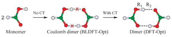
Schematic depiction of two of the computational steps used in the energy decomposition analysis for the formic acid dimer. In the first step, molecular geometries are optimized using block-localized density functional theory (BLDFT-Opt) in which charge densities are constrained within each monomer, whereas charge transfer (CT) effects are included in the second step in which the dimer geometry is fully optimized using the standard delocalized density functional theory (DFT-Opt).
Computed energetic and geometrical results using the BLW-ED method with the hybrid B3LYP DFT are given in Tables 1 and 2, in which three different basis sets were used to examine the dependence of the energy decomposition results on the size of basis functions. The three basis sets are denoted as BS1 for 6-31G(d), BS2 for 6-311+G(d,p), and BS3 for cc-pVTZ. Table 2 shows that there is a small basis set dependence on the optimized donor and acceptor distances, which also contributes to the energy difference with different basis functions in Table 1. Overall, the effect of basis functions on the energy components is small for the formic acid dimer as that found in other complexes.68,70,72,75,163,164 If the same geometries were used in the BLW-ED analysis with different basis sets, the energy variation would have been even smaller.
Table 1.
Computed energy components (kJ mol−1) at the molecular geometries optimized using block-localized density functional theory for the charge-constrained Coulomb complex (BLDFT-Opt), and using the standard density functional theory for the fully delocalized formic acid dimer (DFT-Opt). All calculations are performed using the hybrid B3LYP functional with the 6-31G(d) (BS1), 6-311+G(d,p) (BS2), and cc-pVTZ (BS3) basis sets, respectively
| BLDFT-Opt |
DFT-Opt |
|||||
|---|---|---|---|---|---|---|
| Energy term | BS1 | BS2 | BS3 | BS1 | BS2 | BS3 |
| Δ E def | 1.4 | 1.8 | 1.8 | 12.8 | 10.4 | 13.9 |
| Δ E HL | −23.7 | −27.1 | −24.6 | 6.1 | 6.9 | 18.5 |
| Δ E pol | −11.4 | −12.5 | −13.1 | −32.0 | −32.2 | −41.0 |
| Δ E CT | / | / | / | −50.2 | −44.4 | −53.2 |
| Δ E b | −33.7 | −37.8 | −35.9 | −63.3 | −59.4 | −61.8 |
Table 2.
Optimized donor (R1) and acceptor (R2) hydrogen bond distances (Å), and O–H stretching vibrational frequencies (cm−1) along with the corresponding intensities (kM mol−1) for the charge-constrained Coulomb complex (BLDFT-Opt), for the fully delocalized formic acid dimer (DFT-Opt), and for the monomer. All calculations are performed using the hybrid B3LYP functional with the 6-31G(d) (BS1), 6-311+G(d,p) (BS2), and cc-pVTZ (BS3) basis sets, respectively
| Monomer |
Coulomb complex (BLDFT-Opt) |
Dimer (DFT-Opt) |
|||||||
|---|---|---|---|---|---|---|---|---|---|
| Property | BS1 | BS2 | BS3 | BS1 | BS2 | BS3 | BS1 | BS2 | BS3 |
| R 1 | 0.978 | 0.971 | 0.970 | 0.979 | 0.975 | 0.973 | 1.005 | 0.998 | 1.003 |
| R 2 | / | / | / | 2.014 | 2.047 | 2.024 | 1.691 | 1.704 | 1.659 |
| ν(O–H) | 3700 | 3769 | 3758 | 3646, 3707 | 3674, 3732 | 3668, 3731 | 3127, 3226 | 3163, 3276 | 3077, 3177 |
| Intensity | 0.98 | 1.51 | 1.37 | 4.43, 6.92 | 4.77, 8.24 | 5.22, 9.08 | 2.19, 43.12 | 3.66, 47.04 | 2.41, 50.16 |
Table 1 shows that the coulombic complex of the formic acid dimer would be considerably stable with a binding energy of about −35 kJ mol−1 from BLDFT calculations without electron transfer delocalization between the monomers. The stabilization energy may be attributed to the local dipole–dipole attractions between the two monomers, of which −24 to −27 kJ mol−1 originate from the permanent (unpolarized) charge distribution and −11 to −13 kJ mol−1 from mutual polarization. The hydrogen bond distance, H⋯O (R2), between the two monomers shows a modest dependence on the basis set, varying from 2.014Å to 2.047Å. The O–H stretching frequency shows a red shift of 24–66 cm−1 (note that there are two absorption peaks for the dimer as a result of symmetric and antisymmetric coupling), and the computed absorption intensity is noticeably increased relative to that of the monomer.
Electronic delocalization between the two monomers in the formic acid dimer has a dramatic impact on the optimized hydrogen bond distance in full DFT calculations, with the acceptor H⋯O distance shortened by more than 0.3Å (Table 2), whereas the effect on the donor distance (R1) is rather small. Although we have not investigated if the geometrical changes are artefacts due to the specific functional used, the structural change is nevertheless reflected by marked increases in deformation energy of the individual formic acid, in the Pauli repulsion between the monomers, resulting in a net positive Heitler–London energy term (Table 1). However, they are more than offset by the enhanced polarization and the inclusion of charge transfer stabilization. Table 2 shows that the electronic delocalization from the carbonyl oxygen atom in one monomer to the σOH* in the other greatly weakens the donor O–H bond order, resulting in a remarkable red shift in the O–H stretching frequency by 500–600 cm−1 in comparison with the value of the monomer. Furthermore, the absorption intensity is also significantly increased.
To visualize the effects of polarization and electron transfer on a molecular wave function in intermolecular interactions, we illustrate the change in electron density induced by mutual polarization, and then, by electron transfer. The electron density difference (EDD) isosurfaces are shown in Fig. 2 for the formic acid dimer. The EDD map due to polarization effect is obtained by taking the difference between the total electrons densities of the unpolarized monomer wave function (ψBLW0) and the optimal BLW (ψBLW), both at the geometry of the Coulomb complex optimized using BLDFT (Fig. 1). Similarly, the effect of electron transfer on the molecular wave function is depicted by the difference between the total electron density from the fully delocalized Kohn–Sham orbitals in the standard DFT method and that from the block-localized DFT calculations. Fig. 2a shows that polarization results in electron density shifts predominantly from the hydroxyl hydrogen atom to the carbonyl oxygen atom within each monomer, apparently through π-conjugation. The polarization electron density variation is an important mechanism through which electron transfer is shown in Fig. 2b to occur across the hydrogen bonds in the direction from the carbonyl oxygen atom in one monomer to the hydroxyl hydrogen atom in the other monomer.
Fig. 2.
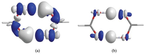
Electron density difference (EDD) isosurfaces showing (a) polarization effects within each monomer in the presence of the electric field of the interacting partner, and (b) electron transfer between the formic acid monomers as a result of delocalization from the block-localized to the fully extended Kohn–Sham orbitals in density functional theory calculations at the B3LYP/6-311+G(d,p) level. Contour levels are shown at 0.001 a.u. (electron per cubic bohr) with white surfaces representing an increase in electron density and black a decrease in electron density. Note that the EDD isosurface is used for qualitative purpose and the size of the density isosurface should not be used as a measure of the magnitude of the density change, akin to the inadequacy of weighing a lead ball and a mushroom by inspection.
The above application of the BLW-ED to the formic acid dimer shows that the BLW-ED approach, making use of block-localized density functional theory, not only can provide quantitative results on the individual energy components, but also can yield unique and rich information on structural and physical properties for the intermediate state where the electron transfer is quenched.
3.2 Cation–π interactions
Because of the exceptionally strong non-covalent interactions, cation–π complexes have long been recognized to play a critical role in biomolecular recognition.165,166 In fact, a variety of cations have been found in close proximity of aromatic sidechains,167–170 suggesting that proteins may use cation–π interactions to bind cationic substrates.171 An understanding of the origin of cation–π interactions is valuable to dissecting the mechanisms of enzymatic catalysis involving ionic substrates172–174 and ion transport.175,176 We have modeled the cation–π interaction in δ-opioid receptor–ligand binding by considering a series of nonbonded complexes involving N-substituted piperidines and substituted monocyclic aromatics.177 Of significance is that the BLW-ED analysis revealed a linear relationship between the total interaction energy and its energy components for these complexes. This finding helps to explain the dilemma that on the one hand simple electrostatic models without the explicit treatment of polarization and charge transfer can model biomolecules with reasonable success, but on the other hand it is well recognized that both polarization and charge-transfer terms play significant roles in cation–π interactions.
Benzene is a prototypical model to illustrate cation–π interactions, which has no net charge and molecular dipole moment. Thus, electrostatic interactions in a cation–π complex have been assumed to be primarily due to quadrupole moment of the aromatic system.171,178–180 Additional many-body terms, including induction, dispersion and charge transfer also make important contributions to cation–π interactions.181 It has been shown that molecular mechanics models with the inclusion of explicit polarization terms can yield better agreement with experiment on cation–π complexes than pair-wise potentials.182,183 The BLW-ED method at the DFT level has been applied to a series of cation–π interactions between cations (Li+, Na+, K+, NH4+ and N(CH3)4+) and benzene (Scheme 1), where the electrostatic and Pauli repulsion energies have been grouped into a single Heitler–London energy term.75 In this article, we employ HF/6-311G(d,p) to further analyze the individual contributions of the electrostatic and Pauli energy terms in these five typical cation–π systems.
Scheme 1.
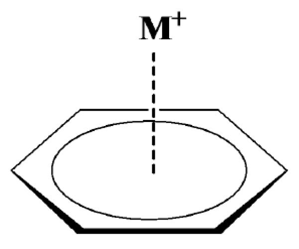
Table 3 lists the computed energy components along with the optimized distances between the cation and benzene centers; in addition, dispersion energy is included at the MP2/6-311G(d,p) level (except for the N(CH3)4+−C6H6 complex in which 6-31G(d) is employed). Geometries and binding energies for the alkali metal ion complexes with benzene have been addressed by Nicholas et al. at various levels,184 and our optimizations yield similar results. In particular, cation–benzene separations are found to be 1.89 (1.87), 2.47 (2.42) and 2.98 (2.81)Å for Li+, Na+ and K+ at the HF/6-311G(d,p) (MP2/6-311G(d,p)) level, respectively, whereas the distances from the nitrogen atom for NH4+ and N(CH3)4+ are 3.12 (2.89) and 4.58 (4.23)Å, respectively. In all cases, inclusion of electron correlation reduces the M+–benzene separation, notably in the cases of K+, NH4+ and N(CH3)4+; the importance of dispersion effects follows the order Li+ < Na+ < K+ < NH4+ < N(CH3)4+.
Table 3.
Optimized ion–benzene separations (angstroms), energy components, and the total binding energies (kJ mol−1), along with experimental enthalpy of binding for benzene–cation complexes from block-localized density functional theory using HF/6-311G(d,p). The dispersion correlation energies are determined at the MP2/6-311G(d,p) level for all complexes except that for the tetramethylammonium ion in which the 6-31G(d) basis is used
| Cation | R | Δ E def | Δ E ele | Δ E ex | Δ E pol | Δ E CT | Δ E disp | Δ E b | ΔH (exp) |
|---|---|---|---|---|---|---|---|---|---|
| Li+ | 1.89 | 1.1 | −88.0 | 50.5 | −85.0 | −39.3 | −2.7 | −163.4 | −160.2a |
| Na+ | 2.47 | 1.2 | −73.0 | 28.8 | −43.4 | −10.7 | −3.0 | −100.1 | −117.2b |
| K+ | 2.98 | 1.0 | −54.7 | 22.8 | −25.7 | −8.2 | −14.6 | −79.4 | −80.3c |
| NH4+ | 3.12 | 1.8 | −52.5 | 25.3 | −23.8 | −10.8 | −17.9 | −77.9 | −80.8d |
| N(CH3)4+ | 4.58 | 0.6 | −21.0 | 7.3 | −5.4 | −5.6 | −18.0 | −42.1 | −39.3e |
Table 3 lists both Coulomb attraction and Pauli exchange repulsion terms. Although the Coulomb interactions are strongly attractive, in the order of Li+ > Na+ > K+ ≈ NH4+ > N(CH3)4+, as the distance between the cation and the benzene plane increases, they are largely offset by short range repulsions as a result of orthogonalization of the block-localized orbitals to satisfy the Pauli Principle. Consequently, the Heitler–London energy, which consists of the Coulomb and Pauli energy terms, follows the order of NH4+ < N(CH3)4+ < K+ < Li+ < Na+ which accounts for 23% (Li+), 44% (Na+), 40% (K+), 35% (NH4+) and 32% (N(CH3)4+) the overall binding energy in each complex. The non-uniform correlation between the electrostatic component and the total binding energy makes it difficult to design a simple pair-wise potential that includes only Coulomb terms to simultaneously yield good agreement in binding energy and geometry in comparison with ab initio results.182
Table 3 reveals that the most significant contribution to benzene–cation binding is polarization in the alkali metal complexes, which dominantly originates from the distortion of the molecular wave function of benzene. For the three alkali cation–benzene complexes, the polarization energy contributes 52%, 43% and 32% to the total binding energies for Li+, Na+ and K+, respectively. It is interesting to note that the polarization effect decreases roughly exponentially with increasing cation–benzene distance. This finding supports previous arguments that the explicit inclusion of polarization in molecular interaction potential is essential to modeling cation–π interactions.182,183,190,191 Without the inclusion of the polarization effect, even the modified OPLS potential that reproduces the quadrupole moment of benzene still just yields a binding enthalpy of −98 kJ mol−1 for the Li+−benzene complex.182 Cubero et al.190 estimated a polarization stabilization energy of −41 kJ mol−1 for the interaction of Na+ with benzene, which is in good agreement with the BLW-ED analysis (−43 kJ mol−1).
To elucidate the origin of polarization effects, the individual contributions from the cation, the in-plane σ bonds and the perpendicular π orbitals of benzene are considered. Each individual polarization contribution is obtained by optimizing the corresponding orbitals, while the remaining block-localized orbitals are kept frozen. In addition, we have partitioned the cation–π system into three blocks, called BLW(3), corresponding to the cation, the σ-framework, and the π-conjugated system to account for the mutual polarization effects, but excluding σ–π coupling. The sums of the three separate contributions are −32.8, −13.1, −6.4, −5.7, and −1.2 kJ mol−1 for the five complexes of Li+, Na+, K+, NH4+, and N(CH3)4+, respectively, which are close to the results from BLW(3) calculations (Table 4). The small difference reflects the mutual polarization effects from the three (cation, σ, and π orbitals) independent components. However, if the σ and π orbitals are grouped in the same fragment to be polarized by a cation, a major enhancement in polarization effect is obtained (the difference between the last two columns in Table 4), ranging from −54.1 for Li+(C6H6) to −3.2 kJ mol−1 for the distant hydrophobic cation N(CH3)4+ (C6H6) complex. The large energy contributions from σ–π coupling in the electronic polarization of benzene is essential to the understanding of cation–π interactions, which cannot be properly modeled by empirical potentials based on dipole polarizability models.
Table 4.
Individual polarization energies for cation and benzene (kJ mol−1)
| Complex | M+ | π(C6H6) | σ(C6H6) | BLW-DFT(3) | C6H6 |
|---|---|---|---|---|---|
| Li+ (C6H6) | −0.04 | −6.32 | −26.40 | −30.63 | −84.73 |
| Na+ (C6H6) | −0.08 | −2.30 | −10.67 | −12.93 | −43.14 |
| K+ (C6H6) | −0.21 | −1.00 | −5.15 | −6.61 | −24.89 |
| NH4+ (C6H6) | −0.38 | −0.96 | −4.35 | −6.02 | −22.64 |
| N(CH3)4+ (C6H6) | −0.42 | −0.08 | −0.71 | −1.38 | −4.60 |
The σ–π coupling in the electronic polarization of benzene can be visualized in the EDD isosurfaces. Shown in Fig. 3a is the change in electron density due to polarization of benzene in the electrical field of Li+. Electronic polarization is evidently due to σ→π* transition, and the overall change is seen as a mushroom cloud effect as the electron density of benzene flushes from the hydrogen atoms through the σCH orbitals into the highly polarized, delocalized π* orbitals of carbon atoms. Other cations have similar effects, although the external field effect decreases as the cation–benzene distance increases. The difference among the cations can also be confirmed by the natural population analysis.192 The electrical field of the alkali cations shifts 0.258e (Li+), 0.186e (Na+) and 0.138e (K+) 0.132e (NH4+) and 0.006e (N(CH3)4+) from the benzene hydrogen atoms into carbon atoms.
Fig. 3.
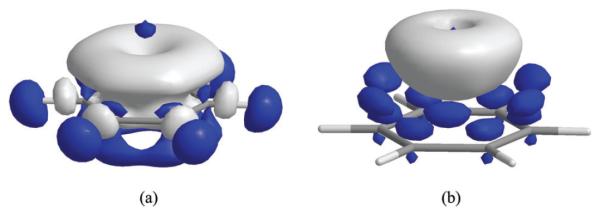
Electron density difference (EDD) isosurface for the Li+(C6H6) complex, depicting (a) polarization effects (contour level at 0.002 a.u.) and (b) charge transfer effects (contour level at 0.001 a.u.) from the BLW-ED analysis at the HF/6-311G(d,p) level.
Interestingly, Fig. 3b reveals that the electron density accumulated on the side of the benzene ring facing the cations is transferred into the cation site. Thus, the overall picture of electronic reorganization in a cation–π complex is the transfer of electron density from the in-plane hydrogen atoms into the perpendicularly positioned cation through σ–π coupling of the benzene orbitals. In this case, polarization and charge transfer effects operate in the same direction to enhance electron density migration.
The BLW-ED analysis demonstrates that charge transfer effects are important and not negligible in cation–π interactions (Table 3 and Fig. 3), particularly for the small ion Li+, in which charge transfer stabilizes the Li+⋯benzene complex by −39.3 kJ mol−1 (compared with −37.2 kJ mol−1 at the DFT level),75 which accounts for 24% of the binding energy. For other cations, charge transfer effect is not as large as in Li+(C6H6), but still makes sizable contribution of more than 10% to the total binding energy. Population analysis reveals that benzene transfers 0.028e, 0.014e, 0.010e, 0.014e and 0.008e to Li+, Na+, K+, NH4+ and N(CH3)4+, respectively. It is interesting to note that although the energetic contributions from charge transfer effects are significant, the net amount of charge transferred from benzene to the cations, in fact, is negligibly small from natural population analysis.
3.3 Transition metal complexes
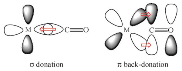
The BLW-ED method provides an excellent venue for studying chemical bonding in metal complexes such as the metal π–ligand bond,34,193 which is found in a wide range of materials, catalysts and fuel cells. Here, we illustrate an application to a series of metal–carbon monoxide complexes. The metal–CO bonding interactions have been extensively investigated and the experimental observations of the CO vibrational frequency shifts and variations in metal–ligand bond distance can be well explained by the Dewar–Chatt–Duncanson model.194–199 Based on this theory, there are two synergic interactions (Scheme 2); one is the σ dative bond from the lone pair electrons of C to the transition metal, and the other is the back-donation from a d orbital of the metal center into the virtual π* orbital of the ligand. Because of the opposite directions in electron flow in σ bonding and dπ back-donation, both interactions are mutually enhanced in the process. It is of great interest to evaluate these two kinds of interactions separately, along with the coupling of the forward and backward electronic flow. Typically, the back-donation from the metal center dominates the mutual interactions, resulting in net electron transfer from the metal to the ligand,200,201 resulting in a reduced CO bond order and an increase in bond length, evidenced by the observation of a red-shift in the C–O stretching frequency. However, in other complexes, the C–O stretch frequencies have been found to be close or blue-shifted relative to that of an isolated carbon monoxide. Bagus et al. used the CSOV method to estimate the energy contributions from various types of bonding to the metal–carbonyl bond.14,202,203 It was found that the CO σ donation contributes just about one third of the bonding interactions compared with that due to dπ back-donation. This differs from the analysis by Blyholder and Lawless who separated the total energy into monatomic and diatomic energy terms at the semi-empirical level, resulting in a conclusion that σ bonding is more important.199
Scheme 2.
We have used the BLW-ED method to probe the properties of chemical bonding in transition metal–CO complexes, including the neutral MCO (M = Ni, Pd, Pt) and cationic M+CO (M+ = Cu+, Ag+, Au+) species using block-localized density functional theory with the B3LYP functional and the SBKJC valence double-zeta basis with compact relativistic effective core potentials (SBKJC/ECP) for the transition metals204 and the 6-311+G(d) basis set for C and O.205 Structural and energetic results are summarized in Tables 5–7.206 Head-Gordon, Bell and coworkers have also investigated some of these transition metal–CO complexes.207
Table 5.
Optimized bond distances (Å) and vibrational frequencies of CO (cm−1) for the MCO complexes, (M = Ni, Pd, Pt, Cu+ , Ag+ and Au+), using delocalized and block-localized density functional theories. In BLW-DFT calculations, the complex is partitioned into two blocks, corresponding to a transition metal and carbon monoxide, respectively. The SBKJC split valence basis with an effective core potential is used for transition metals and the 6-311+G(d) basis is used for carbon and oxygena
| DFT |
BLW-DFT |
|||||||
|---|---|---|---|---|---|---|---|---|
| M | R MC | R CO | ν CO | Δ ν CO b | R MC | R CO | ν CO | Δ ν CO a |
| Ni | 1.672 | 1.151 | 2079 | −133 | 2.044 | 1.120 | 2293 | +81 |
| Pd | 1.879 | 1.142 | 2112 | −100 | 2.406 | 1.123 | 2257 | +45 |
| Pt | 1.791 | 1.146 | 2120 | −92 | 2.360 | 1.121 | 2280 | +68 |
| Cu+ | 1.884 | 1.116 | 2316 | +104 | 2.177 | 1.114 | 2342 | +130 |
| Ag+ | 2.199 | 1.116 | 2314 | +102 | 2.570 | 1.117 | 2307 | +95 |
| Au+ | 1.968 | 1.116 | 2310 | +98 | 2.517 | 1.116 | 2320 | +108 |
The equilibrium distance and stretching vibrational frequency for CO are 1.127 Å and 2212 cm−1, respectively, from B3LYP/SBJKC-ECP optimization, which may be compared with the experimental values of 1.128 Å208 and 2143 cm−1.209
Frequency shifts are computed relative to that (2212 cm−1) of a free CO.
Table 7.
Individual polarization energies (ΔEpol) from M and CO, and charge transfer stabilization energies due to σ dative bond ΔECT(σ) and dπ back-donation ΔECT(π)). Energies are given in kJ mol−1
| M | ΔEpol(M) | ΔEpol(CO) |
|
ΔECT(σ) | ΔECT(π) |
|
||
|---|---|---|---|---|---|---|---|---|
| Ni | −48.5 | −39.3 | 2.9 | −94.6 | −204.2 | −12.6 | ||
| Pd | −128.9 | −7.9 | −14.6 | −87.0 | −148.5 | −5.4 | ||
| Pt | −226.4 | −27.2 | −28.0 | −198.3 | −220.1 | −44.4 | ||
| Cu+ | −31.0 | −62.8 | −11.3 | −71.5 | −32.2 | −1.3 | ||
| Ag+ | −15.1 | −37.2 | −4.6 | −63.6 | −14.2 | −0.4 | ||
| Au+ | −68.2 | −50.2 | −17.2 | −172.4 | −53.6 | −13.4 |
.
.
Table 5 shows that without electronic delocalization between the transition metal and CO in BLDFT geometry optimizations, the M–C distances are significantly longer than the equilibrium structure from standard (delocalized) DFT calculations, implicating the key roles of σ-donation and dπ-back bonding interactions. Furthermore, electrostatic polarization of the C=O bond in the presence of the external field of the transition metal enhances the C=O bond order, resulting in a reduction in bond length and a blue-shift of the C–O vibrational frequency in the range of 45 to 130 cm−1 both for the so-called classical and non-classical transition metal–CO complexes. For the neutral species, the exchange repulsion is the dominant force (HL term in Table 6), which is significantly greater than the corresponding polarization stabilization. Thus, electrostatic interactions without covalent bonding interactions through charge delocalization are not sufficient to bring a neutral transition metal and CO together to form a stable complex other than a van der Waals complex. On the other hand, for monocationic complexes, the exchange repulsion is significantly reduced (Table 6), which may be attributed to a more compact electron distribution of the cation, while polarization effects of the CO group are more critical. Surprisingly, Table 6 shows that the polarization energy of the CO group is somewhat greater in the neutral complex than that in the cationic metal center.
Table 6.
Computed energy components in the total binding energies (kJ mol−1) for the transition metal–carbon monoxide complexes using block-localized density functional theory in BLW-ED analysis
| M | Δ E def | Δ E HL | Δ E pol | Δ E CT | Δ E b |
|---|---|---|---|---|---|
| Ni | 3.3 | 113.8 | −84.9 | −311.3 | −279.1 |
| Pd | 1.3 | 232.2 | −151.5 | −241.4 | −159.4 |
| Pt | 2.1 | 438.9 | −281.6 | −462.8 | −303.4 |
| Cu+ | 0.8 | 47.7 | −105.0 | −105.0 | −161.5 |
| Ag+ | 0.8 | 37.2 | −56.9 | −78.2 | −97.1 |
| Au+ | 0.8 | 189.1 | −135.6 | −239.3 | −185.0 |
Relaxation of the block-localized Kohn–Sham orbitals to the fully delocalized, unconstrained DFT calculation drastically increases the covalent character in the M–CO bond, resulting in metal–ligand bond shortening by as large as 0.6 Å and a stabilization energy of more than 460 kJ mol−1 due to charge transfer in the PtCO complex. Interestingly, the overall electronic delocalization effects can be separated into σ donation and dπ back-bonding contributions by specifically block-localizing the corresponding orbitals in BLDFT calculations. The advantage of our BLW-ED analysis is that the energies due to forward and backward electronic donation are variationally optimized as opposed to a perturbative Roothaan step calculation by Khaliullin et al.207 Table 7 reveals that the electronic delocalization stabilization due to orbital mixing between the dπ orbital of the metal with the 2π* orbital of CO ΔECT(π) is noticeably greater for the neutral complexes than the σdonation from the carbon lone pair in CO to the metal dσ orbitals ΔECT(σ). However, not surprisingly, induction effects through σbonding donation from the ligand to the metal center are the main factor in the cationic complexes. The reversal of electronic structural interactions between σdonation and dπ back-bonding in the neutral and cationic complexes makes a qualitative difference in the computed CO stretching vibrational frequency shifts. In the neutral complexes, the strong electron back-donation to the 2π* orbital of carbon monoxide significantly weakens the C–O bond, sufficient to overcome the opposite effect due to electronic polarization, leading to an increase in the C–O bond length and −92 to −133 cm−1 red-shifts in the C–O vibrational frequency relative to a free CO. In contrast, back donation is weak in the cationic, “nonclassical metal carbonyl” species and the CO stretching vibrational frequency shifts remain positive in good agreement with experiment.210
In concluding this section, we note that the BLW-ED analysis offers a clear and unified picture for the different trends in the neutral MCO (M = Ni, Pd, Pt) and cationic MCO+ (M+ = Cu+, Ag+, Au+) complexes. While the CO polarization induced by the metals enhances the C–O bond and increases the C–O vibrational frequencies, the π back-donation tends to weaken the C–O bond and decrease the C–O vibrational frequencies. For neutral complexes, the latter is more prominent than the former, thereby resulting in significant red-shifts in the C–O vibrational frequencies. In contrast, σ induction in the direction towards the cation center is most significant, whereas the dπ back-donation is minimal in MCO+ complexes. Consequently, the C–O bonds in the cationic complexes retain higher bond orders thanks to electronic polarization effects and blue-shifted vibrational frequencies relative to the free CO.
4. Prospects
The advantage of the BLW method, expressed both in terms of wave function theory and density functional theory, lies in the definition and self-consistent optimization of the wave function of the intermediate, electron-localized states where polarization and charge transfer among interacting species can be deactivated. While the present energy decomposition approach divides the total intermolecular interaction into a number of physically intuitive terms, including structural deformation, electrostatic, Pauli repulsion, and polarization energy terms, the difference between the optimal results from standard (delocalized) DFT and block-localized DFT computations manifests the changes in structure and physical properties due to charge transfer/delocalization effects among the monomers. Note that our block-localization approach is a general concept, not only applicable to individual molecular fragments, but also to atomic orbitals on the same element such that specific σ and π electronic effects can be analyzed.
The BLW method has been implemented both in the Hartree–Fock theory and in density functional theory. DFT treats dynamic correlations extremely well for compact molecular structures, a major advantage over WFT in computational costs. However, the current functionals developed for the Kohn–Sham DFT are less successful for systems that have a high degree of degeneracy in the electronic structure; here, WFT is more effective in treating static correlations. Although recent advances in DFT-D schemes, in which molecular mechanics terms are introduced to model dispersion interactions, have significantly enhanced the accuracy for treating hydrogen-bonding and van der Waals complexes,211,212 an exploration of methods that go beyond the current Kohn–Sham density functional theory can be useful.
To this end, we have described a multistate density functional theory (MSDFT) in which BLDFT is used to define charge localized, VB-like states, which are used in configuration interaction or multiconfiguration self-consistent field (MCSCF) approaches to obtain the adiabatic ground state energy.1,76 The MSDFT method is an extension of the mixed molecular orbital and valence bond (MOVB) theory that has been extensively used for chemical reactions in solution previously.126–129
Starting from eqn (6), we first define a charge transfer state between monomers a and b by combining these two monomers into a single block:1
| (21) |
where Φab represents a product of molecular orbitals that are constructed using the basis functions of both monomers a and b, is a charge transfer state of the two monomers indexed by the subscript in the electrostatic field of the rest of the system, and N(ab) is a normalization factor. Clearly, there are k − 1 blocks in eqn (21), whereas there are k monomer blocks in eqn (6). Thus, the energy difference between the state specified by eqn (21) and that by eqn (6) can be categorized as the CT energy between monomers a and b in the presence of all other monomers.
| (22) |
To a good approximation, the BLW energy (eqn (7)) plus the sum of all pair-wise CT energies (eqn (22)) provides a first order estimate of the total energy of the supermolecular complex,106 which can be generalized to trimer corrections and higher order terms.1 An advantage of the block-localization followed by pair-wise CT energy corrections is that it divides a large supermolecular calculation into k smaller monomer fragmental calculations,72–74,106 which naturally leads to a linear-scaling approach as the number of monomer blocks increases.213–217
The resonance of all dimeric charge transfer states defined by eqn (21), which accounts for the overall charge delocalization effects in the entire supermolecular complex, can be represented by the following multistate wave function:1
where the subscript X2 specifies that the configurational basis functions are the dimeric charge transfer states. Obviously, the extension to many-body CT states is straightforward.1
Two computational approaches have been described.77 In the first method, each CT diabatic state is first variationally optimized and then used in configuration interaction calculations. Here, only the configurational coefficients are optimized and this procedure is called the variational diabatic configuration (VDC) method.77,126–128 Alternatively, in the second method, both configurational and orbital coefficients in all states are consistently optimized in the same fashion as in MCSCF theory. The latter approach is called the consistent diabatic state (CDC) method.77
In MOVB, either using VDC or CDC, the configurational matrix elements are given as follows:
| (24) |
where the subscripts u and w specify, respectively, a given CT state defined by eqn (21), and J and K are matrices of the Coulomb and Exchange integrals. Importantly, eqn (24) is equally applicable to MSDFT, with the only exception that the exchange integral K is replaced by the exchange-correlation potential, Exc[ρuw(r)]:76
| (25) |
where the density, both for the same state (u = w) and exchange transition state (u≠w), is given generally as follows:
| (26) |
where Cu and Cw are the coefficient matrices of occupied orbitals for state functions and .
The expression in eqn (23) is a multistate generalization of the single determinant Kohn–Sham theory, which is used to define and generate the electron densities for the individual block-localized states. The difference, however, is that the total electron density specified by eqn (23) is not directly used to determine the adiabatic ground state energy; rather, the latter is obtained by a multistate self-consistent field procedure. This differs conceptually and computationally from the ensemble DFT218 and the works of Filatov and Shaik219,220 and Baerends and coworkers221 in that the coupling of different configurational states is included. In fact, the generalization of eqn (25) to density functional theory is a key result of MSDFT. An advantage of MSDFT is that the difficult task of imposing the necessary constraints to a single determinant to obtain the exact ground state electron density is separated into constraining densities corresponding to VB-like configurational states. Consequently, MSDFT takes advantages of both the excellent performance of KSDFT in the treatment of dynamic correlation and the convenience of multistate configuration interaction to model static correlation.
A number of issues remain to be addressed. The current functionals developed for the Kohn–Sham DFT approach may not be suited for such a multistate density functional approach since the adiabatic ground state energy is not computed from a single, optimized ground state density, as opposed to the KSDFT algorithm. However, the KSDFT approach is used to determine the energies and matrix elements of block-localized configurational states. Thus, these functionals are in principle applicable to BLDFT calculations, which has been shown to be a rigorously defined constrained DFT (CDFT).76 The use of a multiconfigurational approach within density functional theory has the suspicion that there is a double counting of electron correlation effects. This is a subject that still requires careful examination and testing. Nevertheless, the block-localization procedure constrains electron distribution corresponding to a given Lewis structure, which naturally introduces nodes into the wave function. Thus, it is expected that static electron correlations due to configuration mixing are also reduced or removed from such a constrained DFT approach, which are subsequently recovered from the configuration interaction or MCSCF procedure.
In concluding this perspective, we use the minimum energy configuration of the water trimer complex to illustrate an application of MSDFT, in comparison with the results using MOVB in WFT, to elucidate the origin of the trimer interaction energy. Table 8 lists the computed relative energies for the strictly monomer-localized state , for the pair-wise charge transfer states , and for the resonance delocalized configuration (ΘX2) corresponding to the adiabatic ground state. Both WFT and DFT are examined; we note that the multistate approach using WFT is called the mixed molecular orbital and valence bond theory (MOVB) which has been used in a variety of applications and applied to the explicit polarization (X-Pol) method as a generalized (GX-Pol) theory,126–129 whereas it is called MSDFT76 using density functional theory to define block-localized states. In the latter method, the popular PBE0 and B3LYP functionals are employed.217,222
Table 8.
Computed relative energies (kJ mol−1 ) for the minimum energy structure of a water trimer using MOVB and MSDFT with PBE0 and B3LYP functionals. All calculations are performed using the aug-cc-pCVDZ basis set at the HF/6-31+G(d) geometry
| Method | MOVBa | MSDFT/PBE0b | MSDFT/B3LYPb | |
|---|---|---|---|---|
|
|
0.00 | 0.0 | 0.0 | |
|
|
−36.2 | −40.8 | −34.0 | |
|
|
−4.7 | −8.0 | −8.5 | |
|
|
−4.1 | −6.7 | −7.1 | |
|
|
−4.6 | −7.7 | −8.2 | |
|
|
−49.5 | −63.2 | −57.7 | |
| Δ E HF/DFT | −49.2 | −63.1 | −57.5 | |
| VDC (3) | −43.5 | −53.2 | −47.1 | |
| CDC (3) | −58.7 | −63.1 | −57.3 |
This work.
The Hartree–Fock, PBE0, and B3LYP total energies of the three isolated water molecules are, respectively, −228.12879, −229.08669, −229.23051 a.u., using the cc-pCVDZ basis set.
The energy of the monomeric block-localized configuration relative to the three separated water molecules is the total electrostatic interaction energy, including mutual polarization without charge transfer, which are determined to be −36.2, −40.8, and −34.0 kJ mol−1 using HF and DFT with the PBE0 and B3LYP functions, respectively. The states yield the three pair-wise charge transfer energies in the water trimer complex, which amounts to −4.1 to −4.7 kJ mol−1 in the HF theory, and −6.7 to −8.5 kJ mol−1 in DFT. CT makes significant contributions to the total interaction energy of the water trimer complex. Noticeably, the numerical results from the present energy decomposition analysis show that there is a greater CT effect using DFT than using WFT. The total interaction energies ΔEHF/DFT are −49.2, −63.1, and −57.5 kJ mol−1 at the HF, DFT/PBE0 and DFT/B3LYP levels of theory, respectively, in which the inclusion of electron correlation in the latter two methods greatly enhances binding interactions. Remarkably, the sum of the total electrostatic and the three pair-wise CT energies yields nearly an identical result as that from calculations of the full system for all three methods, suggesting a powerful decomposition procedure in which the total interaction energy of a full system may be estimated, to a high degree of accuracy, by summing up the monomer and dimer block-localized energies in the presence of the remainder of the system.156
The resonance delocalization energy of the dimeric CT states, , can be obtained either through the VDC or through the CDC procedure, accounting for the coupling effects among the three VB-like diabatic states. Clearly, it is critical to relax the charge densities of different states in the multiconfiguration, multistate optimizations, without which only about 56% of the total charge transfer effects are obtained in the three-configuration VDC(3) calculations. On the other hand, the interaction energy from the multistate MOVB/CDC(3) approach is significantly enhanced; the amount of energy exceeding the full Hartree–Fock results may be assigned to correlation effects, which is −9.5 kJ mol−1 in the water trimer structure. It is of interest to note that the MSDFT results with three CT states, using the PBE0 and B3LYP functionals, essentially reproduced the full DFT interaction energies. This is a further affirmation that the likelihood of double counting of electron correlation effects is minimal in the MSDFT method, making use of the current approximate functionals in KSDFT to define the block-localized configuration states. In this regard, it is important to notice that the dimeric “CT” energies from DFT calculations in Table 2, in fact, have contributions both from the charge delocalization effect as that illustrated in the MOVB theory and from the recovery of electron correlation from the three-block constrained state to a two-block constrained configuration. If we use the difference between the DFT dimeric CT energy and that of the HF-MOVB CT energy as a rough estimate of the correlation energy in the state relative to the fully monomer constrained , the sum of the dimer-correlation energies are −9.0 and −10.4 kJ mol−1, a value very similar to the correlation energy (−9.5 kJ mol−1) from MOVB/CDC(3) estimate. As a result, the total interaction energies from the MOVB/CDC(3) and the MSDFT calculations are found to be in good agreement (the last row in Table 8), yet, the origin of the energy terms from these methods are quite different. The results show that the MSDFT method can provide valuable insights that would otherwise be extremely difficult to infer from the delocalized KSDFT model.
Acknowledgements
This work has been partially supported by the National Institutes of Health (Grant GM46736) and the National Science Foundation (Grant CHE09-57162).
Biographies
 Yirong Mo
Yirong Mo received his PhD in Physical Chemistry in 1992 from Xiamen University, China. His PhD work concerns the development of the ab initio VB theory. He was a DAAD Visiting Fellow and a Humboldt Research Fellow in Germany in 1996–1997, when he started to develop the BLW method. Later he worked with Professor Jiali Gao on the combined QM(MOVB)/MM method and MD simulations of enzymatic catalysis. After one-year tenure at Xencor Inc., he joined the Western Michigan University in 2002. His research interests include the electron transfer theory and the modeling and engineering of biological systems.
 Peng Bao
Peng Bao received a B.S. in Chemistry from Tsinghua University in 1996 and a M.S. in Organic Chemistry from Lanzhou University in 1999. After doing new drug synthesis in a Pharmaceutical Company, he realized his interests are in theoretical and computational chemistry. He studied at the Institute of Chemistry, Chinese Academy of Sciences (ICCAS), and obtained a Ph.D. in 2007 under the direction of Prof. Zhongheng Yu. After graduation, he joined the faculty at ICCAS and became Associate Professor in 2009. Currently, he is a postdoctoral associate with Prof. Jiali Gao at University of Minnesota. His research interests include theoretical studies of intermolecular and intramolecular interactions, and the modeling of macromolecular systems.
 Jiali Gao
Jiali Gao obtained a B.S. degree from Beijing University and a Ph.D. in 1987 at Purdue University. He was on the faculty of Chemistry at the State University of New York, Buffalo, from 1990 through 1999. He moved to the University of Minnesota in 2000, where he is currently the Lee I. Smith Professor of Chemistry. His research interests include development and applications of quantum chemical methods for macromolecular systems. He developed the first fragmental block-localized quantum mechanical method in 1997, called the explicit polarization (X-Pol) theory, to treat condensed phase and macromolecular systems as a next-generation force field. Recently, he proposed the concept of analytical coarse graining (ACG) of macromolecular particles for modeling processes in biological cells.
References
- 1.Gao J, Cembran A, Mo Y. J. Chem. Theor. Comput. 2010;6:2402–2410. doi: 10.1021/ct100292g. [DOI] [PubMed] [Google Scholar]
- 2.Halperin I, Ma BY, Wolfson H, Nussinov R. Proteins: Struct., Funct., Genet. 2002;47:409–443. doi: 10.1002/prot.10115. [DOI] [PubMed] [Google Scholar]
- 3.Jorgensen WL. Science. 2004;303:1813–1818. doi: 10.1126/science.1096361. [DOI] [PubMed] [Google Scholar]
- 4.Colizzi F, Perozzo R, Scapozza L, Recanatini M, Cavalli A. J. Am. Chem. Soc. 2010;132:7361–7371. doi: 10.1021/ja100259r. [DOI] [PubMed] [Google Scholar]
- 5.Hao GF, Yang GF, Zhan CG. J. Phys. Chem. B. 2010;114:9663–9676. doi: 10.1021/jp102546s. [DOI] [PMC free article] [PubMed] [Google Scholar]
- 6.Bolon DN, Mayo SL. Proc. Natl. Acad. Sci. U. S. A. 2001;98:14274–14279. doi: 10.1073/pnas.251555398. [DOI] [PMC free article] [PubMed] [Google Scholar]
- 7.Alexandrova AN, Rothlisberger D, Baker D, Jorgensen WL. J. Am. Chem. Soc. 2008;130:15907–15915. doi: 10.1021/ja804040s. [DOI] [PMC free article] [PubMed] [Google Scholar]
- 8.Jiang L, Althoff EA, Clemente FR, Doyle L, Röthlisberger D, Zanghellini A, Gallaher JL, Betker JL, Tanaka F, Barbas CF, Hilvert D, Houk KN, Stoddard BL, Baker D. Science. 2008;319:1387–1391. doi: 10.1126/science.1152692. [DOI] [PMC free article] [PubMed] [Google Scholar]
- 9.Siegel JB, Zanghellini A, Lovick HM, Kiss G, Lambert AR, St Clair JL, Gallaher JL, Hilvert D, Gelb MH, Stoddard BL, Houk KN, Michael FE, Baker D. Science. 2010;329:309–313. doi: 10.1126/science.1190239. [DOI] [PMC free article] [PubMed] [Google Scholar]
- 10.Morokuma K. J. Chem. Phys. 1971;55:1236–1244. [Google Scholar]
- 11.Kitaura K, Morokuma K. Int. J. Quantum Chem. 1976;10:325–340. [Google Scholar]
- 12.Morokuma K. Acc. Chem. Res. 1977;10:294–300. [Google Scholar]
- 13.Ziegler T, Rauk A. Theor. Chem. Acc. 1977;46:1–10. [Google Scholar]
- 14.Bagus PS, Hermann K, Bauschlicher CW., Jr J. Chem. Phys. 1984;80:4378–4386. [Google Scholar]
- 15.Stevens WJ, Fink WH. Chem. Phys. Lett. 1987;139:15–22. [Google Scholar]
- 16.Glendening ED, Streitwieser A. J. Chem. Phys. 1994;100:2900–2909. [Google Scholar]
- 17.Chen W, Gordon MS. J. Phys. Chem. 1996;100:14316–14328. [Google Scholar]
- 18.van der Vaart A, Merz KM., Jr J. Phys. Chem. A. 1999;103:3321–3329. [Google Scholar]
- 19.Reinhardt P, Piquemal J-P, Savin A. J. Chem. Theor. Comput. 2008;4:2020–2029. doi: 10.1021/ct800242n. [DOI] [PubMed] [Google Scholar]
- 20.Wu Q, Ayers PW, Zhang YK. J. Chem. Phys. 2009;131:164112. doi: 10.1063/1.3253797. [DOI] [PubMed] [Google Scholar]
- 21.Su P, Li H. J. Chem. Phys. 2009;131:014101. doi: 10.1063/1.3159673. [DOI] [PubMed] [Google Scholar]
- 22.Boys SF, Bernardi F. Mol. Phys. 1970;19:553–566. [Google Scholar]
- 23.Scheiner S. Hydrogen Bonding: A Theoretical Perspective. Oxford University Press; New York: 1997. [Google Scholar]
- 24.Bagus PS, Illas F. J. Chem. Phys. 1992;96:8962–8970. [Google Scholar]
- 25.Márquez AM, López N, García-Hernández M, Illas F. Surf. Sci. 1999;442:463–476. [Google Scholar]
- 26.Piquemal J-P, Márquez A, Parisel O, Giessner-Prettre C. J. Comput. Chem. 2005;26:1052–1062. doi: 10.1002/jcc.20242. [DOI] [PubMed] [Google Scholar]
- 27.Gourlaouen C, Piquemal J-P, Saue T, Parisel O. J. Comput. Chem. 2006;27:142–156. doi: 10.1002/jcc.20329. [DOI] [PubMed] [Google Scholar]
- 28.Reed AE, Curtiss LA, Weinhold F. Chem. Rev. 1988;88:899–926. [Google Scholar]
- 29.Reed AE, Weinhold F. Isr. J. Chem. 1991;31:277–285. [Google Scholar]
- 30.Glendening ED. J. Phys. Chem. A. 2005;109:11936–11940. doi: 10.1021/jp058209s. [DOI] [PubMed] [Google Scholar]
- 31.Dapprich S, Frenking G. J. Phys. Chem. 1995;99:9352–9362. [Google Scholar]
- 32.Bickelhaupt FM, Baerends EJ. In: Rev. Comp. Chem. Lipkowitz KB, Boyd DB, editors. vol. 15. Wiley-VCH; New York: 1999. p. 1. [Google Scholar]
- 33.te Velde GT, Bickelhaupt FM, Baerends EJ, Guerra CFS, Van Gisbergen JA, Snijders JG, Ziegler T. J. Comput. Chem. 2001;22:931–967. [Google Scholar]
- 34.Frenking G, Frohlich N. Chem. Rev. 2000;100:717–774. doi: 10.1021/cr980401l. [DOI] [PubMed] [Google Scholar]
- 35.Bickelhaupt FM, Baerends EJ. Angew. Chem., Int. Ed. 2003;42:4183–4188. doi: 10.1002/anie.200350947. [DOI] [PubMed] [Google Scholar]
- 36.Kovács A, Esterhuysen C, Frenking G. Chem.-Eur. J. 2005;11:1813–1825. doi: 10.1002/chem.200400525. [DOI] [PubMed] [Google Scholar]
- 37.Michalak A, Mitoraj M, Ziegler T. J. Phys. Chem. A. 2008;112:1933–1939. doi: 10.1021/jp075460u. [DOI] [PubMed] [Google Scholar]
- 38.Mitoraj MP, Michalak A, Ziegler T. J. Chem. Theor. Comput. 2009;5:962–975. doi: 10.1021/ct800503d. [DOI] [PubMed] [Google Scholar]
- 39.Dederichs PH, Bluegel S, Zeller R, Akai H. Phys. Rev. Lett. 1984;53:2512–2515. doi: 10.1103/PhysRevLett.56.2407. [DOI] [PubMed] [Google Scholar]
- 40.Allen LC. Chem. Phys. Lett. 1968;2:597–601. [Google Scholar]
- 41.Francisco E, Martín Pendás A, Blanco MA. J. Chem. Theor. Comput. 2006;2:90–102. doi: 10.1021/ct0502209. [DOI] [PubMed] [Google Scholar]
- 42.Korchowiec J, Uchimaru T. J. Chem. Phys. 2000;112:1623–1633. [Google Scholar]
- 43.Mayer I, Hamza A. Int. J. Quantum Chem. 2005;103:798–807. [Google Scholar]
- 44.Liu S, Govind N. J. Phys. Chem. A. 2008;112:6690–6699. doi: 10.1021/jp800376a. [DOI] [PubMed] [Google Scholar]
- 45.Diner S, Malrieu JP, Claverie P. Theor. Chem. Acc. 1969;13:1–17. [Google Scholar]
- 46.Diner S, Malrieu JP, Jordan F, Gilbert M. Theor. Chem. Acc. 1969;15:100–110. [Google Scholar]
- 47.Hayes IC, Stone AJ. Mol. Phys. 1984;53:83–105. [Google Scholar]
- 48.Stone AJ. The Theory of Intermolecular Forces. Oxford University Press; New York: 1996. [Google Scholar]
- 49.Szalewicz K, Jeziorski B. Mol. Phys. 1979;38:191–208. [Google Scholar]
- 50.Chalasiński G, Szczesniak MM. Mol. Phys. 1988;63:205–224. [Google Scholar]
- 51.Jeziorski B, Moszynski R, Szalewicz K. Chem. Rev. 1994;94:1887–1930. [Google Scholar]
- 52.Williams HL, Chabalowski CF. J. Phys. Chem. A. 2001;105:646–659. [Google Scholar]
- 53.Heßelmann A, Jansen G. Chem. Phys. Lett. 2002;357:464–470. [Google Scholar]
- 54.Wells BH, Wilson S. Chem. Phys. Lett. 1983;101:429–434. [Google Scholar]
- 55.Xantheas SS. J. Chem. Phys. 1996;104:8821–8824. [Google Scholar]
- 56.Angeli C, Cimiraglia R, Malrieu JP. J. Chem. Educ. 2008;85:150–158. [Google Scholar]
- 57.Guihéry N, Malrieu JP, Evangelisti S, Maynau D. Chem. Phys. Lett. 2001;349:555–561. [Google Scholar]
- 58.Malrieu JP, Guihéry N, Calzado CJ, Angeli C. J. Comput. Chem. 2006;28:35–50. doi: 10.1002/jcc.20546. [DOI] [PubMed] [Google Scholar]
- 59.Lewis GN. J. Am. Chem. Soc. 1916;38:762–785. [Google Scholar]
- 60.Special Issue. J. Comput. Chem. 2007;28(1):1–466. [Google Scholar]
- 61.Pauling LC. The Nature of the Chemical Bond. 3rd edn Cornell University Press; Ithaca, NY: 1960. [Google Scholar]
- 62.Wheland GW. Resonance in Organic Chemistry. Wiley & Sons; New York: 1955. [Google Scholar]
- 63.Cooper DL. Valence Bond Theory. Elsevier; Amsterdam: 2002. [Google Scholar]
- 64.Gallup GA. Valence Bond Methods: Theory and Applications. Cambridge University Press; New York: 2002. [Google Scholar]
- 65.Shaik SS, Hiberty PC. A Chemist's Guide to Valence Bond Theory. Wiley-Interscience; New York: 2007. [Google Scholar]
- 66.Mo Y, Peyerimhoff SD. J. Chem. Phys. 1998;109:1687–1697. [Google Scholar]
- 67.Mo Y. J. Chem. Phys. 2003;119:1300–1306. [Google Scholar]
- 68.Mo Y, Schleyer P. v. R. Chem.–Eur. J. 2006;12:2009–2020. [Google Scholar]
- 69.Mo Y, Song L, Wu W, Cao Z, Zhang Q. J. Theor. Comput. Chem. 2002;1:137–151. [Google Scholar]
- 70.Mo Y, Gao J. Acc. Chem. Res. 2007;40:113–119. doi: 10.1021/ar068073w. [DOI] [PubMed] [Google Scholar]
- 71.Mo Y. Nat. Chem. 2010;2:666–671. doi: 10.1038/nchem.721. [DOI] [PubMed] [Google Scholar]
- 72.Mo Y, Gao J, Peyerimhoff SD. J. Chem. Phys. 2000;112:5530–5538. [Google Scholar]
- 73.Mo Y, Gao J. J. Phys. Chem. A. 2001;105:6530–6536. [Google Scholar]
- 74.Mo Y, Gao J. J. Phys. Chem. B. 2006;110:2976–2980. doi: 10.1021/jp057017u. [DOI] [PubMed] [Google Scholar]
- 75.Mo Y, Song L, Lin Y. J. Phys. Chem. A. 2007;111:8291–8301. doi: 10.1021/jp0724065. [DOI] [PubMed] [Google Scholar]
- 76.Cembran A, Song L, Mo Y, Gao J. J. Chem. Theor. Comput. 2009;5:2702–2716. doi: 10.1021/ct9002898. [DOI] [PMC free article] [PubMed] [Google Scholar]
- 77.Song L, Gao J. J. Phys. Chem. A. 2008;120:12925–12935. doi: 10.1021/jp803050e. [DOI] [PMC free article] [PubMed] [Google Scholar]
- 78.Valero R, Song L, Gao J, Truhlar DG. J. Chem. Theor. Comput. 2009;5:1–22. doi: 10.1021/ct800318h. [DOI] [PMC free article] [PubMed] [Google Scholar]
- 79.Khaliullin RZ, Cobar EA, Lochan RC, Bell AT, Head-Gordon M. J. Phys. Chem. A. 2007;111:8753–8765. doi: 10.1021/jp073685z. [DOI] [PubMed] [Google Scholar]
- 80.Banks JL, Kaminski GA, Zhou RH, Mainz DT, Berne BJ, Friesner RA. J. Chem. Phys. 1999;110:741–754. [Google Scholar]
- 81.Chelli R, Procacci P. J. Chem. Phys. 2002;117:9175–9189. [Google Scholar]
- 82.Yang ZZ, Wu Y, Zhao DX. J. Chem. Phys. 2004;120:2541–2557. doi: 10.1063/1.1640345. [DOI] [PubMed] [Google Scholar]
- 83.Anisimov VM, Lamoureux G, Vorobyov IV, Huang N, Roux B, MacKerell AD. J. Chem. Theor. Comput. 2005;1:153–168. doi: 10.1021/ct049930p. [DOI] [PubMed] [Google Scholar]
- 84.Kaminski GA, Ponomarev SY, Liu AB. J. Chem. Theor. Comput. 2009;5:2935–2943. doi: 10.1021/ct900409p. [DOI] [PMC free article] [PubMed] [Google Scholar]
- 85.Borodin O. J. Phys. Chem. B. 2009;113:11463–11478. doi: 10.1021/jp905220k. [DOI] [PubMed] [Google Scholar]
- 86.Zhao DX, Liu C, Wang FF, Yu CY, Gong LD, Liu SB, Yang ZZ. J. Chem. Theor. Comput. 2010;6:795–804. doi: 10.1021/ct9006647. [DOI] [PubMed] [Google Scholar]
- 87.Wu JC, Piquemal J-P, Chaudret R, Reinhardt P, Ren P. J. Chem. Theor. Comput. 2010;6:2059–2070. doi: 10.1021/ct100091j. [DOI] [PMC free article] [PubMed] [Google Scholar]
- 88.Gao J, Pavelites JJ, Habibollahzadeh D. J. Phys. Chem. 1996;100:2689–2697. [Google Scholar]
- 89.van Lenthe JH, Balint-Kurti GG. Chem. Phys. Lett. 1980;76:138–142. [Google Scholar]
- 90.van Lenthe JH, Balint-Kurti GG. J. Chem. Phys. 1983;76:5699–5713. [Google Scholar]
- 91.Cooper DL, Gerratt J, Raimondi M. Nature. 1986;323:699–701. [Google Scholar]
- 92.Cooper DL, Gerratt J, Raimondi M. Chem. Rev. 1991;91:929–964. [Google Scholar]
- 93.Hiberty PC. THEOCHEM. 1997:398–399. 35–43. [Google Scholar]
- 94.Thorsteinsson T, Cooper DL. J. Math. Chem. 1998;23:105–126. [Google Scholar]
- 95.Wu W, Wu A, Mo Y, Lin M, Zhang Q. Int. J. Quantum Chem. 1998;67:287–297. [Google Scholar]
- 96.Mcweeny R. Int. J. Quantum Chem. 1999;74:87–96. [Google Scholar]
- 97.Dijkstra F, van Lenthe JH. J. Chem. Phys. 2000;113:2100–2108. [Google Scholar]
- 98.Song L, Mo Y, Zhang Q, Wu W. J. Comput. Chem. 2005;26:514–521. doi: 10.1002/jcc.20187. [DOI] [PubMed] [Google Scholar]
- 99.Hiberty PC, Shaik S. J. Comput. Chem. 2007;28:137–151. doi: 10.1002/jcc.20478. [DOI] [PubMed] [Google Scholar]
- 100.Song L, Song J, Mo Y, Wu W. J. Comput. Chem. 2009;30:399–406. doi: 10.1002/jcc.21065. [DOI] [PubMed] [Google Scholar]
- 101.Goddard WAI. Phys. Rev. 1967;157:73–80. [Google Scholar]
- 102.Bobrowicz FW, Goddard WA., III . In: Methods of Electronic Structure Theory. Schaefer HF III, editor. Plenum; New York: 1977. pp. 79–127. [Google Scholar]
- 103.McWeeny R. Proc. R. Soc. London, Ser. A. 1959;253:242–259. [Google Scholar]
- 104.Mulliken RS, Parr RG. J. Chem. Phys. 1951;19:1271–1278. [Google Scholar]
- 105.Sovers OJ, Kern CW, Pitzer RM, Karplus M. J. Chem. Phys. 1968;49:2592–2599. [Google Scholar]
- 106.Stoll H, Preuss H. Theor. Chim. Acta. 1977;46:11–21. [Google Scholar]
- 107.Stoll H, Wagenblast G, Preuss H. Theor. Chim. Acta. 1980;57:169–178. [Google Scholar]
- 108.Kollmar H. J. Am. Chem. Soc. 1979;101:4832–4840. [Google Scholar]
- 109.Daudey JP, Trinquier G, Barthelat JC, Malrieu JP. Tetrahedron. 1980;36:3399–3401. [Google Scholar]
- 110.Mehler EL. J. Chem. Phys. 1977;67:2728–2739. [Google Scholar]
- 111.Mehler EL. J. Chem. Phys. 1981;74:6298–6306. [Google Scholar]
- 112.Fülscher MP, Mehler EL. J. Comput. Chem. 1981;12:811–828. [Google Scholar]
- 113.Famulari A, Gianinetti E, Raimondi M, Sironi M. Int. J. Quantum Chem. 1998;69:151–158. [Google Scholar]
- 114.Gianinetti E, Raimondi M, Tornaghi E. Int. J. Quantum Chem. 1996;60:157–166. [Google Scholar]
- 115.Gianinetti E, Vandoni I, Famulari A, Raimondi M. Adv. Quantum Chem. 1998;31:251–266. [Google Scholar]
- 116.Famulari A, Specchio R, Gianinetti E, Raimondi M. In: Valence Bond Theory. Cooper DL, editor. vol. 10. Elsevier; Amsterdam: 2002. p. 313. [Google Scholar]
- 117.Kohn W. Rev. Mod. Phys. 1998;71:1253–1266. [Google Scholar]
- 118.Kohn W, Sham LJ. Phys. Rev. Sect. A. 1965;140:1133–1138. [Google Scholar]
- 119.Zhao Y, Schultz NE, Truhlar DG. J. Chem. Theor. Comput. 2006;2:364–382. doi: 10.1021/ct0502763. [DOI] [PubMed] [Google Scholar]
- 120.Parr RG, Yang W. Density-Functional Theory of Atoms and Molecules. Oxford University Press; New York: 1989. [Google Scholar]
- 121.Frenking G. J. Comput. Chem. 1999;20(1):1–183. [Google Scholar]
- 122.Dułak M, Kaminski JW, Wesolowski TA. J. Chem. Theor. Comput. 2007;3:735–745. doi: 10.1021/ct600367t. [DOI] [PubMed] [Google Scholar]
- 123.Behler J, Delley B, Reuter K, Scheffler M. Phys. Rev. B: Condens. Matter. 2007;75:115409. [Google Scholar]
- 124.Lein M, Szabo A, Kovacs A, Frenking G. Faraday Discuss. 2003;124:365–378. doi: 10.1039/b300066b. [DOI] [PubMed] [Google Scholar]
- 125.Erhardt S, Frenking G. Chem.–Eur. J. 2006;12:4620–4629. doi: 10.1002/chem.200500580. [DOI] [PubMed] [Google Scholar]
- 126.Mo Y, Gao J. J. Comput. Chem. 2000;21:1458–1469. [Google Scholar]
- 127.Mo Y, Gao J. J. Phys. Chem. A. 2000;104:3012–3020. [Google Scholar]
- 128.Gao J, Garcia-Viloca M, Poulsen TD, Mo Y. Adv. Phys. Org. Chem. 2003;38:161–181. [Google Scholar]
- 129.Song L, Mo Y, Gao J. J. Chem. Theor. Comput. 2009;5:174–185. doi: 10.1021/ct800421y. [DOI] [PMC free article] [PubMed] [Google Scholar]
- 130.Gao J, Xia X. Science. 1992;258:631–635. doi: 10.1126/science.1411573. [DOI] [PubMed] [Google Scholar]
- 131.Schmidt MW, Baldridge KK, Boatz JA, Elbert ST, Gordon MS, Jensen JJ, Koseki S, Matsunaga N, Nguyen KA, Su S, Windus TL, Dupuis M, Montgomery JA. J. Comput. Chem. 1993;14:1347–1363. [Google Scholar]
- 132.Jeffrey GA. An Introduction to Hydrogen Bonding. Oxford University Press; New York: 1997. [Google Scholar]
- 133.Desiraju GR, Steiner T. The Weak Hydrogen Bond in Structural Chemistry and Biology. Oxford University Press; New York: 2001. [Google Scholar]
- 134.Isaacs ED, Shukla A, Platzman PM, Hamann DR, Barbiellini B, Tulk CA. Phys. Rev. Lett. 1999;82:600–603. [Google Scholar]
- 135.Tapan KG, Viktor NS, Patrick RK, Ernest RD. J. Am. Chem. Soc. 2000;122:1210–1214. [Google Scholar]
- 136.Grabowski SJ, Sokalski WA, Leszczynski J. J. Phys. Chem. A. 2005;109:4331–4341. doi: 10.1021/jp0444215. [DOI] [PubMed] [Google Scholar]
- 137.Pakiari AH, Eskandari K. THEOCHEM. 2006;759:51–60. [Google Scholar]
- 138.Gilli G, Gilli P. J. Mol. Struct. 2000;552:1–15. [Google Scholar]
- 139.Gilli P, Bertolasi V, Pretto L, Ferretti V, Gilli G. J. Am. Chem. Soc. 2004;126:3845–3855. doi: 10.1021/ja030213z. [DOI] [PubMed] [Google Scholar]
- 140.Gora RW, Grabowski SJ, Leszczynski J. J. Phys. Chem. A. 2005;109:6397–6405. doi: 10.1021/jp044072e. [DOI] [PubMed] [Google Scholar]
- 141.Cleland WW, Kreevoy MM. Science. 1994;264:1887–1890. doi: 10.1126/science.8009219. [DOI] [PubMed] [Google Scholar]
- 142.Frey PA, Whitt SA, Tobin JB. Science. 1994;264:1927–1930. doi: 10.1126/science.7661899. [DOI] [PubMed] [Google Scholar]
- 143.Cleland WW, Frey PA, Gerlt JA. J. Biol. Chem. 1998;273:25529–25532. doi: 10.1074/jbc.273.40.25529. [DOI] [PubMed] [Google Scholar]
- 144.Lough AJ, Park S, Ramachandran R, Morris RH. J. Am. Chem. Soc. 1994;116:8356–8357. [Google Scholar]
- 145.Lee JC, Jr, Peris E, Rheingold AL, Crabtree RH. J. Am. Chem. Soc. 1994;116:11014–11019. [Google Scholar]
- 146.Richardson TB, de Gala S, Crabtree RH, Siegbahn PEM. J. Am. Chem. Soc. 1995;117:12875–12876. [Google Scholar]
- 147.Custelcean R, Jackson JE. Chem. Rev. 2001;101:1963–1980. doi: 10.1021/cr000021b. [DOI] [PubMed] [Google Scholar]
- 148.Gilli G, Bellucci F, Ferretti V, Bertolasi V. J. Am. Chem. Soc. 1989;111:1023–1028. doi: 10.1021/ja00269a047. [DOI] [PubMed] [Google Scholar]
- 149.Bertolasi V, Gilli P, Ferretti V, Gilli G. J. Am. Chem. Soc. 1991;113:4917–4925. [Google Scholar]
- 150.Gilli P, Bertolasi V, Ferretti V, Gilli G. J. Am. Chem. Soc. 2000;122:10405–10417. [Google Scholar]
- 151.Gilli P, Bertolasi V, Pretto L, Lyčka A, Gilli G. J. Am. Chem. Soc. 2002;124:13554–13567. doi: 10.1021/ja020589x. [DOI] [PubMed] [Google Scholar]
- 152.Gordon MS, Jensen JH. Acc. Chem. Res. 1996;29:536–543. [Google Scholar]
- 153.Egli M, Sarkhel S. Acc. Chem. Res. 2007;40:197–205. doi: 10.1021/ar068174u. [DOI] [PubMed] [Google Scholar]
- 154.Pierce AC, Sandretto KL, Bemis GW. Proteins: Struct., Funct., Genet. 2002;49:567–576. doi: 10.1002/prot.10259. [DOI] [PubMed] [Google Scholar]
- 155.Hobza P, Havlas Z. Chem. Rev. 2000;100:4253–4264. doi: 10.1021/cr990050q. [DOI] [PubMed] [Google Scholar]
- 156.Li X, Liu L, Schlegel HB. J. Am. Chem. Soc. 2002;124:9639–9647. doi: 10.1021/ja020213j. [DOI] [PubMed] [Google Scholar]
- 157.van der Veken BJ, Herrebout WA, Szostak R, Shchepkin DN, Havlas Z, Hobza P. J. Am. Chem. Soc. 2001;123:12290–12293. doi: 10.1021/ja010915t. [DOI] [PubMed] [Google Scholar]
- 158.Thompson WH, Hynes JT. J. Am. Chem. Soc. 2000;122:6278–6286. [Google Scholar]
- 159.Pejov L, Hermansson K. J. Chem. Phys. 2003;119:313–324. [Google Scholar]
- 160.Joseph J, Jemmis ED. J. Am. Chem. Soc. 2007;129:4620–4632. doi: 10.1021/ja067545z. [DOI] [PubMed] [Google Scholar]
- 161.Mo Y. J. Mol. Model. 2006;12:665–672. doi: 10.1007/s00894-005-0021-y. [DOI] [PubMed] [Google Scholar]
- 162.Beck JF, Mo Y. J. Comput. Chem. 2007;28:455–466. doi: 10.1002/jcc.20523. [DOI] [PubMed] [Google Scholar]
- 163.Mo Y. J. Phys. Chem. A. 2009;113:5163–5169. doi: 10.1021/jp808941h. [DOI] [PubMed] [Google Scholar]
- 164.Mo Y, Hiberty PC, Schleyer P. v. R. Theor. Chem. Acc. 2010;127:27–38. [Google Scholar]
- 165.Ma JC, Dougherty DA. Chem. Rev. 1997;97:1303–1324. doi: 10.1021/cr9603744. [DOI] [PubMed] [Google Scholar]
- 166.Sussman JL, Harel M, Frolow F, Oefner C, Goldman A, Toker L, Silman I. Science. 1991;253:872–879. doi: 10.1126/science.1678899. [DOI] [PubMed] [Google Scholar]
- 167.Daopin S, Sauer U, Nicholson H, Matthews BW. Biochemistry. 1991;30:7142–7153. doi: 10.1021/bi00243a015. [DOI] [PubMed] [Google Scholar]
- 168.Hendsch ZS, Tidor B. Protein Sci. 1994;3:211–226. doi: 10.1002/pro.5560030206. [DOI] [PMC free article] [PubMed] [Google Scholar]
- 169.Waldburger CD, Schildbach JF, Sauer RT. Nat. Struct. Biol. 1995;2:122–128. doi: 10.1038/nsb0295-122. [DOI] [PubMed] [Google Scholar]
- 170.Cabarcos OM, Weinheimer CJ, Lisy JM. J. Chem. Phys. 1998;108:5151–5154. [Google Scholar]
- 171.Dougherty DA. Science. 1996;271:163–168. doi: 10.1126/science.271.5246.163. [DOI] [PubMed] [Google Scholar]
- 172.Stauffer DA, Barrans JRE, Dougherty DA. Angew. Chem., Int. Ed. Engl. 1990;29:915–918. [Google Scholar]
- 173.McCurdy A, Jiménez L, Stauffer DA, Dougherty DA. J. Am. Chem. Soc. 1992;114:10314–10321. [Google Scholar]
- 174.Shi Z, Butel CJ, Griffin JH. Proc. Natl. Acad. Sci. U. S. A. 1994;91:7370–7274. doi: 10.1073/pnas.91.15.7370. [DOI] [PMC free article] [PubMed] [Google Scholar]
- 175.Kumpf RA, Dougherty DA. Science. 1993;261:1708–1710. doi: 10.1126/science.8378771. [DOI] [PubMed] [Google Scholar]
- 176.Mecozzi S, West AP, Dougherty DA. Proc. Natl. Acad. Sci. U. S. A. 1996;93:10566–10571. doi: 10.1073/pnas.93.20.10566. [DOI] [PMC free article] [PubMed] [Google Scholar]
- 177.Mo Y, Subramanian G, Ferguson DM, Gao J. J. Am. Chem. Soc. 2002;124:4832–4837. doi: 10.1021/ja0174433. [DOI] [PubMed] [Google Scholar]
- 178.Mecozzi S, West AP, Dougherty DA. J. Am. Chem. Soc. 1996;118:2307–2308. [Google Scholar]
- 179.Gentle IR, Ritchie GLD. J. Phys. Chem. 1989;93:7740–7744. [Google Scholar]
- 180.Craven IE, Hesling MR, Laver DR, Lukins PB, Ritchie GLD, Vrbancich J. J. Phys. Chem. 1989;93:627–631. [Google Scholar]
- 181.Kim KS, Lee JY, Lee SJ, Ha T-H, Kim DH. J. Am. Chem. Soc. 1994;116:7399–7400. [Google Scholar]
- 182.Caldwell JW, Kollman PA. J. Am. Chem. Soc. 1995;117:4177–4178. [Google Scholar]
- 183.Eriksson MAL, Morgantini PY, Kollman PA. J. Phys. Chem. B. 1999;103:4474–4480. [Google Scholar]
- 184.Nicholas JB, Hay BP, Dixon DA. J. Phys. Chem. A. 1999;103:1394–1400. [Google Scholar]
- 185.Taft RW, Anvia F, Gal JF, Walsh S, Capon M, Holmes MC, Hosn K, Olumi G, Vasanwala R, Yazdani S. Pure Appl. Chem. 1990;62:17–23. [Google Scholar]
- 186.Guo BC, Purnell JW, Castleman AW. Chem. Phys. Lett. 1990;168:155–160. [Google Scholar]
- 187.Sunner J, Nishizawa K, Kebarle P. J. Phys. Chem. 1981;85:1814–1820. [Google Scholar]
- 188.Deakyne CA, Meot-Ner M. J. Am. Chem. Soc. 1985;107:474–479. [Google Scholar]
- 189.Meot-Ner M, Deakyne CA. J. Am. Chem. Soc. 1985;107:469–474. [Google Scholar]
- 190.Cubero E, Luque FJ, Orozco M. Proc. Natl. Acad. Sci. U. S. A. 1998;95:5976–5980. doi: 10.1073/pnas.95.11.5976. [DOI] [PMC free article] [PubMed] [Google Scholar]
- 191.Cubero E, Orozco M, Luque FJ. J. Phys. Chem. A. 1999;103:315–321. [Google Scholar]
- 192.Reed AE, Weinstock RB, Weinhold F. J. Chem. Phys. 1984;83:735–746. [Google Scholar]
- 193.Scherer W, Eickerling G, Shorokhov D, Gullo E, McGrady GS, Sirsch P. New J. Chem. 2006;30:309–312. [Google Scholar]
- 194.Dewar MJS. Bull. Soc. Chim. Fr. 1951;18:C71–C79. [Google Scholar]
- 195.Chatt JT, Duncanson LA. J. Chem. Soc. 1953:2939–2947. [Google Scholar]
- 196.Mason R. Nature. 1968;217:543–545. [Google Scholar]
- 197.Blyholder G. J. Phys. Chem. 1964;68:2772–2777. [Google Scholar]
- 198.Blyholder G. J. Mol. Catal. A: Chem. 1997;119:11–17. [Google Scholar]
- 199.Blyholder G, Lawless M. J. Am. Chem. Soc. 1992;114:5828–5832. [Google Scholar]
- 200.Bagus PS, Nelin CJ, Bauschlicher CW., Jr Phys. Rev. B: Condens. Matter. 1983;28:5423–5438. doi: 10.1103/physrevb.35.441. [DOI] [PubMed] [Google Scholar]
- 201.Lupinetti AJ, Frenking G, Strauss SH. Angew. Chem., Int. Ed. 1998;37:2113–2116. doi: 10.1002/(SICI)1521-3773(19980817)37:15<2113::AID-ANIE2113>3.0.CO;2-2. [DOI] [PubMed] [Google Scholar]
- 202.Bagus PS, Hermann K, Bauschlicher CW., Jr J. Chem. Phys. 1984;81:1966–1974. [Google Scholar]
- 203.Bauschlicher CW, Jr, Bagus PS, Roos BO. J. Chem. Phys. 1986;85:354–364. [Google Scholar]
- 204.Stevens WJ, Krauss M, Basch H, Jasien PG. Can. J. Chem. 1992;70:612–630. [Google Scholar]
- 205.Krishnan R, Binkley JS, Seeger R, Pople JA. J. Chem. Phys. 1980;72:650–654. [Google Scholar]
- 206.Nakashima K, Zhang X, Xiang M, Lin Y, Lin M, Mo Y. J. Theor. Comput. Chem. 2008;7:639–654. [Google Scholar]
- 207.Khaliullin RZ, Bell AT, Head-Gordon M. J. Chem. Phys. 2008;128:184112. doi: 10.1063/1.2912041. [DOI] [PubMed] [Google Scholar]
- 208.Gilliam OR, Johnson CM, Gordy W. Phys. Rev. 1950;78:140–144. [Google Scholar]
- 209.Huber KP, Herzberg G. Molecular Spectra and Molecular Structure, Constants of Diatomic Molecules 4. Van Nostrand-Reinhold; New York: 1979. [Google Scholar]
- 210.Hurlburt PK, Rack JJ, Luck JS, Dec SF, Webb JD, Anderson OP, Strauss SH. J. Am. Chem. Soc. 1994;116:10003–10014. [Google Scholar]
- 211.Wu Q, Yang W. J. Chem. Phys. 2002;116:515–524. [Google Scholar]
- 212.Grimme S. J. Comput. Chem. 2006;27:1787–1799. doi: 10.1002/jcc.20495. [DOI] [PubMed] [Google Scholar]
- 213.Gao J. J. Phys. Chem. B. 1997;101:657–663. [Google Scholar]
- 214.Gao J. J. Chem. Phys. 1998;109:2346–2354. [Google Scholar]
- 215.Xie W, Gao J. J. Chem. Theor. Comput. 2007;3:1890–1900. doi: 10.1021/ct700167b. [DOI] [PMC free article] [PubMed] [Google Scholar]
- 216.Xie W, Orozco M, Truhlar DG, Gao J. J. Chem. Theor. Comput. 2009;5:459–467. doi: 10.1021/ct800239q. [DOI] [PMC free article] [PubMed] [Google Scholar]
- 217.Perdew JP, Burke K, Ernzerhof M. Phys. Rev. Lett. 1996;77:3865–3868. doi: 10.1103/PhysRevLett.77.3865. [DOI] [PubMed] [Google Scholar]
- 218.Mermin ND. Phys. Rev. Sect. A. 1965;137:A1441–A1443. [Google Scholar]
- 219.Filatov M, Shaik S. Chem. Phys. Lett. 1998;288:689–697. [Google Scholar]
- 220.Filatov M, Shaik S. J. Phys. Chem. A. 2000;104:6628–6636. [Google Scholar]
- 221.Schipper PRT, Gritsenko OV, Baerends EJ. Theor. Chem. Acc. 1998;99:329–343. [Google Scholar]
- 222.Adamo C, Barone V. J. Chem. Phys. 1999;110:6158–6170. [Google Scholar]