Resting-state fMRI in the Human Connectome Project

Stephen M Smith; Jesper Andersson; Edward J Auerbach; Christian F Beckmann; Janine Bijsterbosch; Gwenaëlle Douaud; Eugene Duff; David A Feinberg; Ludovica Griffanti; Michael P Harms; Michael Kelly; Timothy Laumann; Karla L Miller; Steen Moeller; Steve Petersen; Jonathan Power; Gholamreza Salimi-Khorshidi; Abraham Z Snyder; An Vu; Mark W Woolrich; Junqian Xu; Essa Yacoub; Kamil Ugurbil; David Van Essen; Matthew F Glasser; the WU-Minn HCP Consortium

doi:10.1016/j.neuroimage.2013.05.039

. Author manuscript; available in PMC: 2014 Oct 15.

Published in final edited form as: Neuroimage. 2013 May 20;80:144–168. doi: 10.1016/j.neuroimage.2013.05.039

Resting-state fMRI in the Human Connectome Project

Stephen M Smith ^1,^*, Jesper Andersson ¹, Edward J Auerbach ², Christian F Beckmann ³, Janine Bijsterbosch ¹, Gwenaëlle Douaud ¹, Eugene Duff ¹, David A Feinberg ⁴, Ludovica Griffanti ^1,⁵, Michael P Harms ⁶, Michael Kelly ¹, Timothy Laumann ⁶, Karla L Miller ¹, Steen Moeller ², Steve Petersen ⁶, Jonathan Power ⁶, Gholamreza Salimi-Khorshidi ¹, Abraham Z Snyder ⁶, An Vu ^2,⁴, Mark W Woolrich ⁷, Junqian Xu ^2,⁸, Essa Yacoub ², Kamil Ugurbil ², David Van Essen ⁶, Matthew F Glasser ⁶; the WU-Minn HCP Consortium

PMCID: PMC3720828 NIHMSID: NIHMS484858 PMID: 23702415

Abstract

Resting-state functional magnetic resonance imaging (rfMRI) allows one to study functional connectivity in the brain by acquiring fMRI data while subjects lie inactive in the MRI scanner, and taking advantage of the fact that functionally related brain regions spontaneously co-activate. rfMRI is one of the two primary data modalities being acquired for the Human Connectome Project (the other being diffusion MRI). A key objective is to generate a detailed in vivo mapping of functional connectivity in a large cohort of healthy adults (over 1,000 subjects), and to make these datasets freely available for use by the neuroimaging community. In each subject we acquire a total of one hour of whole-brain rfMRI data at 3 Tesla, with a spatial resolution of 2×2×2mm and a temporal resolution of 0.7s, capitalizing on recent developments in slice-accelerated echo-planar imaging. We will also scan a subset of the cohort at higher field strength and resolution. In this paper we outline the work behind, and rationale for, decisions taken regarding the rfMRI data acquisition protocol and pre-processing pipelines, and present some initial results showing data quality and example functional connectivity analyses.

Introduction

The term “connectome” (Sporns et al., 2005) refers to the mapping of connectivity throughout the brain using such imaging modalities as resting-state functional magnetic resonance imaging (rfMRI) and diffusion MRI. rfMRI is used to study connectivity in the brain by acquiring fMRI data from a subject lying “at rest” in the scanner, and utilising the fact that the spontaneous timeseries from functionally related brain regions are correlated (Biswal et al., 1995, Greicius et al., 2003; De Luca et al., 2005; Fox et al., 2005, Fox and Raichle, 2007). Given sufficient quantity and quality of rfMRI data, one is able over time to generate maps of all major functional networks in the brain, as each spontaneously fluctuates in its activation levels (Smith et al., 2009). The simplest analysis methods, based on strength of correlation between the timecourses of any two brain regions, allow one to infer whether the regions are functionally “connected”, although such simple measures are not quantitative.¹ More complex (and, importantly, multivariate) analysis methods such as independent component analysis (ICA - McKeown et al., 1998; Kiviniemi et al., 2003) allow, from a single data-driven analysis, the simultaneous estimation of multiple distinct components, with control over the level of spatial granularity (level of component sub-splitting). However, none of these methods reveal whether connectivity is direct or indirect (Marrelec et al., 2006); indeed, a major problem for rfMRI-based network modelling (and graph theory) occurs if inferences are made that rely on the assumption that correlation between two nodes’ timecourses is unambiguously indicative of a direct connection.

Emerging from the background of general connectivity estimation techniques such as seed-based correlation and ICA, “connectome” mapping often includes two stages: first the identification of a set of “nodes” (through a parcellation of the brain's grey matter), and secondly, estimation of the set of connections or “edges” between these nodes, based on the fMRI timeseries associated with the nodes. In some approaches, the directionality of these connections is estimated, in an attempt to infer how information flows through the network (see detailed discussion and refs in Smith, 2012).

Mapping the connectome is often assumed to begin with the parcellation of grey matter into (often non-overlapping) regions, for example, on the basis of the rfMRI data itself (Flandin et al., 2002; Cohen et al., 2008; Craddock et al., 2011). Ideally, the regions are functionally specialized parcels, within each of which connectivities are relatively homogeneous - all locations within a parcel are assumed to have a similar general pattern of connectivity to locations in the brain outside the parcel. While acknowledging that there can be variations in connectivity across a parcel (van den Heuvel and Hulshoff Pol, 2010; de Reus and van den Heuvel, 2013), one would hope that such variations are smaller than the differences in connection patterns between different parcels, thus rendering the parcellation (and the functional borders implied) meaningful and reproducible. Although researchers contributing to the WU-Minn Human Connectome Project (in this paper referred to simply as “HCP”) accept that any given parcellation of the brain is an oversimplification, it is still a useful tool by which to reduce the data. As a result, brain connectivity can be represented by the manageable “parcellated connectome” (a parcels × parcels matrix), as opposed to the much larger original “dense connectome” (for example, the voxels × voxels matrix). The HCP will make both forms of the estimated connectome available to the research community (along with various versions of the timeseries data, from different stages of our processing pipeline), but we anticipate that it may be the parcellated connectome that will be of most use to neuroscientists, at least until more sophisticated representations of connectivity are developed by the community. It is likely that the HCP will produce more than one parcellation, as we investigate a range of techniques using data from different combinations of imaging modalities.

The goal of the HCP is to generate the most detailed in vivo mapping of functional connectivities in the healthy adult human brain achieved to date in a large cohort (over 1000 subjects, drawn from families with twins and non-twin siblings; Van Essen et al., 2013). We are acquiring a total of one hour of 3T rfMRI data for each subject, with an isometric spatial resolution of 2mm and a temporal resolution of 0.7s, relying on recent developments in multiband accelerated echo-planar imaging. In the following sections we outline the work behind, and rationale for, decisions taken regarding the rfMRI data acquisition protocol and pre-processing pipelines. We briefly describe the spatial pre-processing pipelines (see Glasser et al., 2013 for full details) and then discuss temporal pre-processing in more depth. We present some initial example results showing data quality and example functional connectivity analyses, and end by discussing important outstanding issues. Most of the results shown in this paper use data acquired from 20 of the earliest subjects (all unrelated to each other) scanned during the first quarter (Q1) after the HCP scanning protocol was finalized (“HCP Phase 2”, where “Phase 1” refers to the methods optimization and piloting efforts).

Acquisition protocol for multiband-accelerated rfMRI data

In this section we review and attempt to explain the major decisions taken in setting up the acquisition protocols for the HCP rfMRI data. For more detail on the pulse sequences, see (Ugurbil et al., 2013). The majority of the HCP data is being acquired at 3 Tesla, which we considered to be the field strength currently most suitable for acquiring high quality data reliably from a large cohort of subjects. A subset of 200 HCP subjects will also be scanned at higher field strength. Acquisitions are based on blood oxygen level dependent (BOLD) contrast (Ogawa et al., 1990), using gradient-echo echo-planar imaging (GE EPI - Mansfield, 1977), as this generates, in general, the highest-quality, most robust fMRI data at 3T.

These primary decisions were therefore “safe” choices; however, the HCP decided to follow a more leading-edge approach with respect to the use of “multiband” accelerated EPI. This technique acquires (excites and then reads out) multiple 2D slices simultaneously, in the same time that a single slice is acquired in standard EPI. The slices are then separated from one another during k-space reconstruction, using the different spatial sensitivities of the multiple receive coils (Larkman et al., 2001; Moeller et al., 2010; Setsompop et al., 2012). HCP investigators had shown early on that reducing TR from 3s to 0.4s increased the sensitivity of detection of resting-state signal fluctuation by up to 60% (Feinberg et al., 2010). This result was initially surprising, because the basic single-voxel timeseries detection power is minimally affected by reduction in TR (at least in the range ~0.5-3s), as the simple statistical gain from the increased number of data points is balanced by the loss in signal level (as TR falls below T₁). However, within the achievable acceleration limits, various factors combine to make accelerating fMRI acquisitions highly advantageous, including: the denser temporal sampling of physiological confounds; the importance of temporal degrees-of-freedom for many analysis techniques (such as high-dimensional ICA, or the use of partial correlation in network modelling); and the value of richer temporal characterisation of resting-state fluctuations. Ultimately, high accelerations are limited in SNR by noise introduced by the unaliasing of simultaneously acquired slices (“g-factor noise”) and incomplete slice separation (“L-factor slice leakage”) (Moeller et al., 2012; Ugurbil et al., 2013).

Early HCP piloting utilised a combination of two accelerations – the multiband method described above, and “simultaneous image refocused” (SIR) (Feinberg et al., 2002), the combined technique being referred to as “multiplexed” EPI (Feinberg et al., 2010). SIR excites multiple slices in rapid succession, and their echoes are refocused in a longer single echo train in which gradient switching (and fat saturation) is shared for increased efficiency. By applying distinct shifts in k-space, the echoes remain separated from each other in k-space, and hence images can be separated from each other easily without resorting to parallel imaging. Because the multiband and SIR acceleration techniques are relatively independent of each other, they can be combined, multiplying their respective acceleration factors to achieve much faster imaging. However, the SIR technique requires longer readout times to encode the multiple slices in a single echo train, leading to increased EPI artefacts, including geometric distortions and signal dropouts in regions of high magnetic field inhomogeneity, and to resolution loss in the phase encode direction. These artefacts become worse if higher spatial resolution imaging is targeted; the undesirable prolongation of the echo train length becomes even more pronounced by the necessity to cover additional k-space points to achieve high resolution. This can be counteracted with the use of in-plane accelerations along the phase encode direction, but at the expense of achievable slice acceleration factor (compromising overall TR reduction). Both the slice and in-plane accelerations rely on parallel imaging through the spatial encoding properties of the receive array coil; consequently, they are not independent of each other and the simultaneous use of both reduces the maximum accelerations achievable with either alone. Furthermore, unlike slice accelerations, the use of in-plane acceleration substantially reduces the image SNR due to undersampling penalties. Recently, it has become possible to attain higher slice acceleration factors without the use of the SIR technique. Controlled aliasing (CAIPIRINHA - Breuer et al., 2005) principles can be applied to slice accelerated multiband EPI, following the slice-gradient “blipping” strategy of Nunes et al., (2006), while minimizing the detrimental accrual of phase dispersion along the slice thickness leading to a voxel tilt. Using this new “blipped-CAIPIRINHA” approach (Setsompop et al., 2012) with a further modification to attain full alignment at the center k-space point (Xu et al., 2012), higher spatial resolution rfMRI using multiband EPI was piloted in the HCP. The results suggested that higher spatial resolution fMRI acquisitions were feasible with high accelerations using multiband EPI alone, without the use of in-plane acceleration, and provided advantages over more conventional lower resolution studies. This approach was then adapted for the HCP data acquisition.

Extensive piloting was carried out while the 3T Connectome scanner was at UMinn, to optimise multiband acquisition. In addition, the reconstruction algorithms were improved, to robustly separate (unalias) the simultaneously-acquired slices. A primary question was how much acceleration could be achieved before significant slice-cross-talk occurred, or undesirable artefacts arose in the multiband reconstruction due to interactions with head motion. An initial round of piloting indicated that acceleration between x4 and x8 was optimal, with encouraging results (including reconstruction simulations) up to x8 (Ugurbil et al., 2013).

Another important issue involves the trade-offs between spatial and temporal resolution. There was consensus that voxels should be isometric (cubic), primarily because sampling of fMRI data onto the thin and highly-folded cortical grey matter is only as accurate as the lowest-resolution dimension. We wanted spatial resolution to be as high as possible, subject to two constraints: 1) the smaller the voxels, the (much!) worse the SNR; 2) the smaller the voxels, the worse the temporal resolution (all other things being equal). The drive for higher spatial resolution arises largely from the priority we placed on cortical surface-based analyses of fMRI data, rather than focusing on conventional 3D volumetric analyses. Surface-based analysis reduces blurring across distinct functional areas within individuals when smoothing is required, and results in better cross-subject alignment of functional areas. Accurate 3D-volume to 2D-surface mapping is aided when fMRI data has similar or better resolution than the thickness of the cortical grey matter by reducing partial volume effects with non-grey-matter tissues. Higher resolution also reduces the geometrically induced correlation between neighbouring (touching) banks of a sulcus (or across thin gyral blades of white matter) caused by voxels shared by surface vertices that are close together in 3D, but distant along the surface. This geometric effect is substantially reduced with 2mm data (Glasser et al., 2013).

Pilot studies using a range of resolutions and EPI accelerations indicated that reducing voxel size to less than 2mm was not beneficial at 3T, in terms of the spatial detail discernible in the rfMRI resting-state correlation structure. This was not only due to the reduction in SNR with increased spatial resolution, but also the relatively large point spread function of the BOLD effect at 3T (Parkes et al., 2005), which was measured to be ~3.5mm at full-width-at-half-maximum (FWHM) caused by the dominant draining vein contribution at this field strength (Uludag et al., 2009). Higher spatial resolutions are feasible at higher field strengths, such as 7T, because of increases in image SNR (Vaughan et al., 2001), and in BOLD-based susceptibility contrast (Yacoub et al., 2001); further, at higher fields, the relative contribution of the microvascular-based BOLD signal becomes more significant (Yacoub et al., 2001; Uludag et al., 2009; Ogawa et al., 1993), significantly reducing the point spread function of the BOLD response; an upper limit of 2mm FWHM was measured at 7T (Shmuel et al., 2007). Because of the improved point spread function at 7T, it is likely that there will be further reductions in cross-sulcal and cross-gyral cross-talk with 2mm or higher resolution voxels (although T₂* blurring can become an increasing concern at higher field strength).

Because of concerns regarding possible interactions of multiband acceleration with head motion, a separate piloting study was carried out on the 3T Siemens Verio at FMRIB. This is similar hardware to the HCP 3T Siemens “Connectome Skyra” scanner, the primary difference being less powerful gradient-coils and gradient-amplifier (a difference of much greater significance for diffusion MRI). We acquired resting and task fMRI data in 6 subjects with 4 acquisition protocols, comparing unaccelerated fMRI (3×3×3mm and 2×2×2mm) against multiband x4 and x8 (2×2×2mm).² These four datasets were acquired for each subject twice - once with “normal” amounts of head motion (i.e., asking the subjects to lie as still as possible), and once with “bad” amounts of frequent deliberate head motion, both in terms of amplitude and speeds of motion. The reconstructed “bad motion” data showed increased motion-related artefacts (in both the accelerated and unaccelerated EPI data), but ICA-based artefact removal (see below) was successful in cleaning the bad-motion datasets such that the final resting-state connectivity results were almost indistinguishable from the low-motion results (see Figs S1 and S2). For both task and resting fMRI, effects of interest could be found with at least as high statistical sensitivity in the 2mm accelerated data as with the 3mm unaccelerated data, despite the much smaller voxel volume. The 2mm unaccelerated data resulted in very poor detection of activation and resting-state networks. Multiband x4 and x8 gave similar results (to each other) for simple analyses such as univariate analysis of task data, and low-dimensional ICA; however, as already shown in Feinberg et al., (2010), analyses that depend more strongly on temporal degrees of freedom (e.g., high-dimensional ICA, and network modelling approaches such as partial correlation) see a significant benefit in the increased number of timepoints obtained via the x8 acceleration, compared with x4.

Fig 1 (A) shows estimations of temporal-SNR (tSNR) for the various acquisition protocols tested in the FMRIB multiband motion piloting, using just the “normal head motion” runs. For each resting-fMRI run, and for each protocol, the temporal-SNR image was generated (after motion correction and highpass filtering, but with no spatial smoothing); this was eroded at the brain edge by 3 voxels to exclude edge effects, and the median (across voxels) SNR value computed. This process was repeated after artefact cleanup (using an early version of the ICA-based cleanup described below). The raw tSNR results indicate that both decreasing the voxel size and increasing the acceleration substantially reduce SNR. However, in terms of the effect on simple univariate timeseries statistics, once the increased number of timepoints is taken into account,³ it is clear that the acceleration is of great statistical value, and approximately counters the loss in SNR caused by the increase in spatial resolution; see Fig 1 (B).

Additional evaluations and discussions within the HCP led to the conclusion that using a multiband acceleration factor of x8 on the Connectome Skyra, with a maximal field-of-view (FoV) shift (controlled aliasing factor) of 1/3 along the phase encode direction, across the simultaneously excited and acquired slices, would robustly provide high-quality data allowing accurate reconstruction (including avoiding substantial cross-talk between slices). In the finalised protocol this acceleration is used to acquire 2×2×2mm data with a temporal resolution of 0.72s. While a larger voxel size would result in even faster imaging and better SNR, this choice provides a good overall balance in which both spatial and temporal resolution are a significant improvement compared with conventional rfMRI datasets.

The loss in SNR associated with the relatively high spatial resolution is also ameliorated by the decision to acquire one hour's worth of data from each subject – much more data than is normally acquired in rfMRI studies. In addition to the resulting gain in statistical sensitivity, longer sessions enable analysis of a greater range of spontaneously fluctuating modes of function in “resting” brain networks. The data is acquired in four 15-minute runs split across two imaging sessions. The run duration of 15 minutes was driven in part by practical limitations of raw data size and online image reconstruction at the scanner, but also in order to reduce the probability of subjects inadvertently falling asleep.

The short TR means that the image obtained at each timepoint has very poor grey-white tissue contrast (in addition to the relatively low SNR), due to T₁ saturation. We were therefore concerned that accuracy and robustness of head motion correction and registration to the subject's structural image might suffer. To avoid this problem, we utilize the single-band reference image (“SBRef”) that is acquired at the beginning of each data run to improve image registrations; this has no slice acceleration and no T₁ saturation (its primary purpose is for calibration of the coil sensitivity profiles needed for multiband unaliasing). Because it has improved tissue contrast and SNR, the SBRef image is used as the target image for head motion correction and as the representative fMRI image used to align the fMRI data to the structural data (Glasser et al., 2013). The SBRef is acquired with interleaved slice ordering. No apparent banding artefacts (alternating high and low signal intensity) were observed with the sinc excitation pulse chosen at the Ernst angle of the short TR. Fig 3 shows an example of a raw multiband image and an SBRef reference image.

Fig 3 — Example SBRef and single-timepoint fMRI images, before and after corrections for distortion. Top: SBRef images acquired with L-R phase encoding (left) and R-L phase encoding (right). The central columns are the raw images in native 2mm space; the outer columns are the images after distortion corrections. Middle: equivalent example single-timepoint images from the 4D fMRI timeseries; these are in the same space as the SBRef images, having the same dropout and distortion, but with lower SNR and tissue contrast. The red dilated-brain-edges are the same in all cases, being derived from the average L-R and R-L corrected SBRef images, to allow for easier comparisons across different images. The orange arrows indicate example areas of signal dropout, which are different in L-R and R-L, and are not removed by the distortion corrections. The blue arrows indicate example areas of distortion, which are well corrected by the distortion corrections. Bottom: distortion-corrected SBRef images after alignment to the structural images, with the white-grey boundary (estimated by FreeSurfer from the structural images) overlaid in green. The left-right and right-left phase encoding direction SBRef images are shown separately; there is no obvious residual distortion that is different between these two images. The same corrections are applied to the fMRI timeseries data, which have the same distortions as the SBRef images, but we show just the latter here as the better SNR and tissue contrast make it easier to see the high quality of the alignment to the structural data. The cortical surface overlay views and all surface renderings in following figures were created using the Connectome Workbench display tool (humanconnectome.org/connectome/connectome-workbench.html).

Echo-time (TE) was, after much discussion and evaluation, set to 33ms. Again, this choice is a trade-off; long TE increases BOLD contrast, but decreases overall signal level and increases signal dropout in areas of B₀ inhomogeneity. The TE for optimal functional CNR is equal to T₂* when thermal noise dominates; however, T₂* varies spatially, meaning that no single TE can be optimal throughout the entire brain. Acquiring multiple echoes in a single EPI readout train, or in separate acquisitions with multiple TEs, was not acceptable due to significantly prolonged readout duration and/or TR. Thus, the shortest TE that could be achieved without the use of partial Fourier or in-plane accelerations was selected, to minimize signal dropout. At 2mm resolution, with the Connectome scanner gradients, this TE was 33ms, given the excitation pulse width (~7ms) required to achieve the (Ernst) flip angle (52°) for multiband x8. The use of partial Fourier to reduce TE resulted in larger signal dropouts than acquiring a full Fourier coverage of k-space with longer TEs (likely caused by local phase ramps in regions of B₀ inhomogeneity shifting signal outside the acquired k-space region); hence partial Fourier was not utilised. The EPI echo train length is 52.2ms for the final HCP fMRI protocol. The additional blurring along the phase encode direction due to apparent transverse relaxation (T2* ≈ 45ms) in grey and white matter (Wansapura et al., 1999) in the final HCP fMRI protocol is generally not significant,⁴ except in regions where the T2* is much shorter than the average. We carried out limited piloting to test whether adding small amounts (b ≈ 50s/mm²) of isotropic diffusion weighting (Boxerman et al., 1995; Wong et al., 1995) might reduce contributions from larger draining veins, but the improvements were not significant enough to warrant a longer consequential TE and subsequent reduction in SNR.

EPI phase encoding is commonly applied in the anterior-posterior (A-P) or posterior-anterior (P-A) direction. However, for the HCP, we elected to do phase encoding in the left-right/right-left (L-R/R-L) direction. This was partly to minimise the FoV in the phase-encoding direction, hence minimising the number of lines of k-space (90 lines, echo spacing 0.58ms) and therefore the distortion and blurring. The L-R/R-L phase encoding also enabled a shorter TE because of a reduced echo train length. Additional advantage is achieved through the acquisition of two of the 15-minute runs L-R and the other two R-L, so that regions of dropout differ in the two cases. Consequently, the combined data has fewer areas of more complete signal loss, so a greater total fraction of grey matter can be usefully mapped. Optimal methodology for combining analyses across L-R vs. R-L runs is a matter for further research, but in the short-term, connectivity metrics can simply be averaged (or, for example, timeseries from the different runs concatenated). We determined that distortion-corrected L-R and R-L datasets are, in general, anatomically well aligned with each other, even in regions of different dropout – it is only the dropout that differs.

Accurate EPI distortion correction is very important, given the emphasis on spatial fidelity and resolution in the HCP. We implemented an approach, developed initially for diffusion MRI, which uses spin-echo EPI acquisitions, with the same EPI echo train (i.e., echo spacing, echo train length, slice-gradient blips, etc.) as in gradient-echo EPI. Two such images are collected, in opposite phase-encoding directions, to simultaneously model the non-distorted data (Sotiropoulos et al., 2013). Hence, for fMRI, we acquire six spin-echo images, three with L-R and three with R-L phase-encoding, and feed these into FSL's “Topup” tool, in order to estimate a single fieldmap image (Glasser et al., 2013). We found that this gave equivalently good distortion correction accuracy as with a regular field map, but these images are much faster to acquire than traditional fieldmaps (a few seconds instead of tens of seconds), making this approach less susceptible to within-scan head motion. Examples of the distortion correction can be seen in Fig 3.

The FoV was set to 208mm in the read direction (anterior-posterior), 180mm in the phase encoding direction (L-R or R-L; a 104×90 matrix) and 144mm in the inferior-superior direction (72 slices, meaning that 9 groups of 8 simultaneously-acquired slices were obtained). The four 15-minute rfMRI runs are acquired in the two separate fMRI sessions, following the general counter-balanced ordering: 1) in the first session, 15-minutes R-L phase encoding rfMRI, 15-minutes L-R, and then various task-fMRI runs; 2) in the second session, 15-minutes L-R, 15-minutes R-L, and then task-fMRI. The subjects are asked to lie with eyes open, with “relaxed” fixation on a white cross (on a dark background), think of nothing in particular, and not to fall asleep. The scanner room is darkened. Previous rfMRI studies indicate differences in functional connectivity for eyes-open vs. eyes-closed, but do not indicate one approach as being definitively better than the other (Greicius et al., 2003; Van Dijk et al., 2010). We chose eyes-open in order to minimise the risk of subjects falling asleep during two successive runs. To measure cardiac and respiratory signals, a pulse oximeter and respiratory bellows were fitted to participants prior to the fMRI sessions. Those signals, along with the sync pulse from the scanner, were recorded by the scanner host computer at a sampling rate of 400 Hz. The physiological recordings are synchronized with the onset of the first sync pulse.

Data pre-processing and dissemination – general strategy

HCP rfMRI data will be made publicly available in several forms. The raw timeseries data will be made available (along with associated images, such as those needed to carry out B₀ distortion correction), as some researchers may prefer to apply their own pre-processing. However, we also carry out optimised spatial pre-processing of the raw data, which corrects for various distortions and head motion, and aligns the timeseries data to the structural data and into standard space. The outputs from that spatial (“minimal”) pre-processing will be made publicly available, as a more convenient form of the data than the raw, native-acquisition-space, timeseries data. Finally, we will also apply further pre-processing (“temporal”), which will aim to remove confounds such as the slowest temporal drifts, and structured non-neuronal artefacts. Again, the data output by this final pre-processing will be made available for download, and will be the recommended (default) version for researchers wanting the timeseries data. This version of the data (i.e., spatially and temporally pre-processed) will be fed into future HCP-generated connectome analyses, such as group-averaged dense connectomes, parcellation, and parcellated-connectome generation (for an overview, see Fig 2). In following sections we give a summary of the spatial pre-processing (in brief, as this is covered in much more detail in Glasser et al., 2013), and then a more detailed description of the temporal pre-processing. These pre-processing pipelines are primarily based on tools from FSL, FreeSurfer, and Connectome Workbench's command-line functions.

Fig 2 — Simplified graphical overview of HCP rfMRI data organization and analysis flow, including example generation of dense and parcellated connectomes at the group level. Each subject's 15-minute rfMRI dataset is spatially and temporally pre-processed, resulting in two versions of the pre-processed timeseries data – volumetric (in 3D MNI152 space) and grayordinates (surface vertices plus subcortical and cerebellar grey matter voxels). Either of these standard-space versions of the data can be combined across runs and subjects, but the grayordinate version is more compact (it contains only grey-matter data) and should provide better alignment across subjects than the volumetric version. A simple group-level analysis might concatenate all subjects’ datasets in time; from this, the “dense connectome” of average correlations could be estimated. This can be fed into a parcellation, and from this (via the parcels’ associated mean timeseries estimated from the group timeseries data) one can estimate the “parcellated connectome”.

Spatial pre-processing

The goal of spatial (or “minimal”) pre-processing is to remove spatial artefacts from the data without removing other potentially useful information. Briefly, the functional data are: corrected for spatial distortions caused by gradient nonlinearity; corrected for head motion by registration to the single band reference image; corrected for B₀ distortion; and registered to the T1w structural image. All of the preceding transforms are concatenated, together with the structural-to-MNI nonlinear warp field, and this single resulting warp (per timepoint) is applied to the original timeseries to achieve a single resampling into 2mm MNI space. Finally, global intensity normalization (of the entire 4D dataset by a single scaling factor) is applied, and non-brain voxels are masked out. From this resulting volume timeseries, the data are mapped onto the native mesh cortical surface using a ribbon-constrained approach, which excludes locally noisy voxels as measured by the coefficient of variation. Timeseries are resampled from the original FreeSurfer surface mesh onto a lower resolution registered standard mesh of 2mm average vertex spacing, and regularized with 2mm FWHM surface smoothing. Subcortical grey matter voxels are resampled using a 2mm FWHM Gaussian neighbourhood from individual FreeSurfer derived subcortical parcels to a standard atlas set of subcortical parcels with 2mm voxels. Cortical surface time series and subcortical volume time series are combined into a standard grayordinates space in a CIFTI dense time series file. For full details of the spatial pre-processing pipeline, including overview flowcharts, see (Glasser et al., 2013). For example SBRef and single-timepoint rfMRI images, before and after corrections for distortion, see Fig 3.

Fig 4 shows group-averaged structural and functional images, using data from 20 HCP Phase 2 subjects (20 structural images and 80 rfMRI runs). Images are in MNI152 space, after all of the spatial pre-processing steps described above. The mean SBRef EPI data shows excellent alignment to the mean structural image. SBRef L-R vs. R-L averages show asymmetry in dropout, but very little residual distortion. The multiband-accelerated EPI mean-timeseries images are also shown. The asymmetry in dropout is quantified and shown in the colour overlay, having a maximum difference of approximately 60%. Finally, mean temporal-SNR images are shown, derived from data after the spatial pre-processing and temporal highpass filtering has been applied, and without vs. with ICA-based artefact cleanup (as described below). Fig 5 also shows the group-averaged EPI mean-timeseries, but now averaged in grayordinate space and displayed on the cortical surface. The lowest mean intensity is 20% of the highest, and the 5^th and 95^th percentile intensities are 46% and 96% of the maximum, respectively.

Fig 5 — The multiband-accelerated EPI mean-timeseries images, averaged across 20 subjects (80 rfMRI runs). This is similar to the mean EPI images shown in the previous figure, except that the timeseries are averaged across subjects in grayordinate space and only the cortical surface data are shown. The intensity display is arbitrary units; the highest mean intensity is 5 times greater than the lowest.

Temporal pre-processing and artefact removal

A variety of “temporal” pre-processing steps could be applied after the above approaches for spatial pre-processing. These options include: slice timing correction; simple filtering out of low and/or high temporal frequencies; removal/regression of global mean timeseries (averaged over whole-brain, or grey-matter only, or a combination of white matter and cerebro-spinal fluid); removal of spatio-temporal artefacts such as residual motion artefacts, scanner artefacts (including potential artefacts related to the multiband reconstruction) and non-neuronal physiological artefacts (including cardiac and breathing effects); and frame censoring techniques such as motion scrubbing (Power et al., 2011). Temporal pre-processing is particularly important for resting-state analyses, which rely fundamentally on correlations between different voxels’ timeseries, as these can be corrupted by artefacts that span across multiple voxels. In contrast, task fMRI has the advantage of fitting a pre-specified fixed temporal model, which provides greater robustness against artefactual influences. Hence our overall approach is to attempt to be thorough in removing aspects of the data that can be identified as artefact with reasonably strong specificity, while taking a more minimalist approach to removal of more ambiguous / mixed aspects of the data; for example, we do not apply temporal lowpass filtering (see below), as the highest frequencies cannot be considered to only contain artefact.

Slice-timing correction is a pre-processing step that temporally resamples all timeseries, shifting the timing such that all slices appear as if they were acquired at exactly the same point in time. While this can be valuable for improving the estimation of correlation between functionally connected voxels in different slices, particularly for long TR data, the necessary temporal interpolation unavoidably results in the loss of some high-frequency signal. Furthermore, temporal filtering could make it more difficult to use model-based physiological correction techniques. For the low-TR HCP data, we considered such a correction to be unnecessary, and it is not applied in the temporal pre-processing pipeline.

The HCP pre-processing pipeline is very unaggressive with respect to temporal frequency filtering. Minimal highpass filtering is applied (using the -bptf option in FSL's fslmaths tool), with a “cutoff” of 2000s (i.e., FWHM=2355s; note that data length is 864s/run) and a slow rolloff of the power (of retained frequencies) below that point. The effect of this filter is very similar to simply removing linear trends in the data. Similarly, no lowpass filtering is applied, as there is evidence (van Oort et al., 2013; Feinberg et al., 2010) that valid and useful neuronal-related resting-state signal is present up to at least 0.2Hz, and possibly even up to 0.5Hz (albeit potentially dominated by thermal noise, depending on SNR). The resting-state literature has regularly used the term “low-frequency” (or “1/f”) to describe resting-state signals; however, the higher power seen at lower frequencies (~0.01Hz) compared to higher frequencies (~0.1Hz) is likely caused by the smoothing effects of the haemodynamic responses to neural activation; there is no sharp frequency cut-off beyond which point BOLD fluctuations cease. Simple attempts to deconvolve the effects of the haemodynamics result in a relatively flat frequency response (albeit increasingly noisy at higher frequencies), in the range 0.01-0.2Hz (Niazy et al., 2011). Despite this, some analyses may nonetheless benefit from increasing the effective CNR by lowpass temporal filtering - for example, correlation between two voxels’ timeseries, where effective CNR is low because there has been no averaging of either timeseries across multiple voxels. However, analyses in which multiple voxels’ timeseries are averaged together are less prone to the effects of thermal noise, and hence may be degraded, rather than improved, by any lowpass temporal filtering. Such analyses include: seed-based connectivity where the seed is an extended ROI and the data has been extensively spatially smoothed; ICA; dual-regression; or parcellated connectivity analysis. A final reason for our decision not to apply lowpass temporal filtering, and to apply only very weak highpass temporal filtering, was that it is easy for researchers using HCP pre-processed data to apply more aggressive temporal filtering themselves, before their own resting-state connectivity analyses.

We investigated the use of ICA-based artefact removal, to remove non-neural spatiotemporal components from each (highpass filtered) 15-minute run of rfMRI data. ICA is a powerful approach for decomposition of fMRI data as a summation of “good” and “bad” components, where each component comprises a weighted set of voxels (the component's spatial map), along with a single timeseries that is common to those voxels identified (Beckmann and Smith, 2004). The identification of artefacts ideally should be carried out for each run separately, if the artefacts are not spatially consistent across different runs or subjects. This is particularly true where each run contains enough data to support a relatively high-dimensional ICA decomposition (i.e., a large number of components), such as our 1200 timepoint resting state runs. Once ICA has identified a number of artefactual components, the data can be “cleaned” by subtracting these components from the data.

Until recently, ICA-based artefact removal has not been widely applied; there have not been many methods proposed for accurate automated classification of components into “good” vs. “bad” – necessary in order to know which components to remove from the data. Previous methods (Perlbarg et al., 2007; De Martino et al., 2007; Tohka et al., 2008) used a two-stage approach. The first stage generates, for each component, a feature vector, with each element in the vector being the value of a different “feature” (spatial, temporal or spatiotemporal quantities encoding various aspects of the component), for example, how much of that component's spatial map is concentrated at the edge of the brain, or what fraction of the temporal power spectrum lies in the higher frequencies. In the second stage, the set of features is passed into a multivariate classifier (such as a support vector machine), which predicts the “class” (e.g., good vs. bad) for each component. The classifier needs training, which means that a reasonable number of example ICA components must be hand-labelled as good or bad.

A major limitation of existing approaches is the use of a relatively small set of features. Given the spatial resolution and number of timepoints in conventional rfMRI datasets, a larger number of richer features might not be supported by the overall data quality/quantity. We set out to generate a large number of features (currently 185), covering many kinds of “cues” from components’ spatial maps and timecourses that could help the classifier make accurate decisions. We also developed a more complex classifier approach, using several different classifiers, all fed into a “meta-classifier” - an approach known as stacking. The overall approach is referred to as FIX (FMRIB's ICA-based X-noisifier); the FIX approach and initial results of classification accuracy are described in detail in (Salimi-Khorshidi, in preparation), and the effects of the ICA+FIX cleanup (and optimal methods to remove the bad components from the data) are evaluated in detail in (Griffanti, in preparation).

For HCP data, we implemented the following overall approach. First, apply unaggressive temporal highpass filtering as described above. Next, ICA is run using MELODIC with automatic dimensionality estimation (MELODIC estimates how many components the given quality and quantity of data will support being separated from each other); this dimensionality is limited to a maximum of 250. These components are fed into FIX, which classifies components into “good” vs. “bad”. Bad components are then removed from the data. All of this is run using the volumetric data, rather than the grayordinate version of the data, because many artefacts are inherently 3D and do not respect tissue boundaries. The same set of artefactual processes is then removed from the (already created) grayordinates version of the data, by first applying the same highpass temporal filtering, and then regressing the bad components’ timeseries out. For both volume and surface cleanup, the cleanup is done in a “non-aggressive” manner - both the good and bad component timeseries are regressed into the data, and then the resulting bad spatial maps are multiplied by the associated timeseries and subtracted from the original dataset. Thus, in this non-aggressive approach, only the unique variance associated with the bad components is removed from the data. Applying “aggressive” cleanup means removing all variance associated with the bad components, and not just the unique part, when also taking into account the non-artefact component timeseries. We have taken the more conservative non-aggressive approach to avoid removing variance of interest from the data, with the understanding that our cleanup will be less effective for more global types of noise whose variance is shared across good and bad components (this decision will be revisited in future cleanup investigations). As part of this cleanup, we also used 24 confound timeseries derived from the motion estimation (the 6 rigid-body parameter timeseries, their backwards-looking temporal derivatives, plus all 12 resulting regressors squared - Satterthwaite et al., 2013). The motion parameters have the temporal highpass filtering applied to them and are then regressed out of the data aggressively, as they are not expected to contain variance of interest.

Data from 25 HCP subjects (100 rfMRI runs) were hand-labelled, to train FIX.⁵ The average number of components per 15-minute run estimated by ICA was 229; of these, on average 24 components were hand-classified as “good” and the remainder as “bad”.⁶ Leave-one-subject-out testing of the classifier (i.e., leaving one subjects’ 4 runs out, training FIX on the other 19 subjects, and testing on the 4 runs left out) resulted in a mean accuracy of 99.3% in identifying “good” components correctly, and 99% accuracy in identifying “bad” components correctly (with corresponding median values being 100% and 99.3%). The balance between these two accuracies can be adjusted through the setting of a single controlling parameter; one has the option to choose to give greater importance to the accuracy of identification of good or of bad components. It is likely that an important factor in the very high accuracy of FIX classification is the high HCP data quality (and quantity – number of voxels and timepoints in each run), meaning that ICA is able to do a good job of separating multiple signal and noise components. Examples of good and bad components are shown in Figs 6 and 7, and results showing the effects of the cleanup can be seen in Figs 1, 4, 12, 13, S1 and S2. The cleanup reduces the resting-state network timeseries amplitude by ~30%, but, despite that reduction, does not reduce the effective group-level results (as judged by group-level statistics applied to both RSN spatial maps and network matrices).

Fig 6 — Examples of “bad” (above) and “good” (below) components from ICA applied to a single 15-minute resting-state fMRI session. The component spatial maps are shown (in red/blue, overlaid on the raw fMRI data), as well as the component timecourse and its power spectrum. Insets show expanded views of 3 slices from the spatial maps. The classifications of these particular components are quite clear from looking at the spatial maps and the timecourses, whereas in this case the spectrum of the bad component is not obviously artefactual. This is an example of why different features are important for accurate classification in different components. The display tool (“Melview”, an in-house program developed specifically for this purpose) is a convenient way to visualise and hand-label components, for feeding into the FIX classifier training.

Fig 7 — The hand classification of the 25 HCP subjects was carried out using Connectome Workbench with combined surface and volume visualisation. The volume views looked very similar to those of the “Melview” program. Two examples of Connectome Workbench surface views of two single-run ICA components’ spatial maps are shown. One component is clearly artefactual (above), and the other non-artefactual (below). The combined volume and surface approach was found to be useful for several reasons. 1) Cortical signal of interest is generated from the cortical grey matter ribbon and thus always maps onto the surface as strong and distinct patches of activation. 2) Artifacts often don't map onto the surface or do so irregularly (e.g., more on gyri than sulci). Thus comparison of volume and surface maps is often enough to distinguish good signal from bad. 3) Projection to the surface can make certain artefactual patterns easier to spot (such as artefacts in the axial slice plane).

Fig 12 — Mixed-effects cross-subject group-level spatial maps estimated in volumetric (top) and in grayordinates space (middle and bottom), in both cases thresholded at Z>7. The grayordinates map is shown in the bottom row overlaid on the “midthickness” cortical surface that runs halfway between the outer and inner grey matter boundaries. The same map is shown in the middle row on the “very inflated” cortical surface.

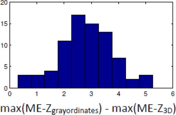
Fig 13 — The increase in peak mixed-effects Z-statistics when carrying out cross-subject group-level analysis in grayordinate space instead of in volumetric MNI standard space. For each RSN from the 100-dimensional group-ICA, the maximum Z-statistic (across space) was computed for both analyses, and the difference between the two maxima computed. The histogram shows the distribution of this difference across RSNs. There is no RSN having a larger mixed-effects Z-statistic peak value in volumetric space. The mean difference (reflecting the extent to which grayordinate-based cross-subject modelling is superior) is 2.8.

Further possible pre-processing steps, such as corrupted-timepoint removal, or global timecourse regression, are still under consideration, and are discussed below. To summarise, the main steps in the temporal pre-processing are:

Data is provided from spatial (“minimal”) pre-processing, in both volumetric and grayordinate forms.
Weak highpass temporal filtering (>2000s FWHM) is applied to both forms, achieving slow drift removal.
MELODIC ICA is applied to volumetric data; artefact components are identified using FIX.
Artefact and motion-related timecourses are regressed out of both volumetric and grayordinate data.
Optionally (and depending on further investigations), possibly also some combination of:
- ○ further motion cleanup / scrubbing;
- ○ further removal of physiological confounds based on physiological monitoring data;
- ○ removal of globally-related signals.

Example connectivity results

Fig 8 shows an example RSN (parts of the DMN – the default mode network) identified by ICA applied to a single 15-minute run from a single subject. ICA was run on the volumetric data, and this non-artefactual component is shown at the top, overlaid onto the single-band reference scan. The ICA timecourses were then regressed into the grayordinate timeseries version of the same dataset, resulting in corresponding spatial maps in grayordinate space; the map matching this component is shown, overlaid on the 20-subject group-average inflated cortical surfaces. In both cases the spatial map is a Z-statistic, mixture-model-corrected⁷ and thresholded at abs(Z)>3. No spatial smoothing was applied to the volumetric data, and apart from the very limited 2mm FWHM spatial smoothing applied to the grayordinate data in the spatial pre-processing pipeline, no further spatial smoothing was applied to the grayordinate data. The level of fine spatial detail and restriction of activation to the grey matter is apparent.

Fig 9 shows a single column from the “dense connectome” - the correlation map from the single seed point (grayordinate) chosen within the default mode network shown in the previous figure. The correlations from this seed to every other point on the cortex are shown for a single-run, a single subject (4 runs concatenated) and 20 subjects (80 runs concatenated). The subject chosen was a “typical” subject, as defined on the basis of parcellated-connectome full correlation matrices at dimensionality of 100 (see below). The group-average matrix was computed, and the subjects ordered according to how similar their within-subject matrix was to the group-average; the median subject was chosen for the examples in this figure.

In Fig 10 we show the detailed spatial specificity of grayordinate-based functional connectivity maps from both a single subject (left) and group average (20 subjects, right). One seed (top row) is a vertex in the retrosplenial cortex, areas 29 and 30. This seed shows strong connectivity throughout the entire retrosplenial cortex and to area POS2 on the anterior bank of the partieto-occipital sulcus (both areas are also defined by their distinct higher myelin content in Glasser and Van Essen (2011) in both hemispheres in both the individual and group average data. The second seed (middle row) is in the neighbouring posterior cingulate cortex (which is more lightly myelinated, Glasser and Van Essen, 2011) and shows connectivity to the default mode network. These very distinct patterns of connectivity are separated by a connectivity gradient in both the individual and group average (bottom row), which has previously been shown to be precisely co-localized with an architectonic gradient in myelin content (Glasser et al., 2011)

Figs 11 and S3 show the group-level ICA spatial maps found by FSL's MELODIC, run on all 20 subjects (80 runs), with ICA dimensionality of 30 and 100 respectively. In both cases (A) shows the original spatial maps from the group-ICA, carried out on the artefact-cleaned grayordinate versions of the fMRI datasets. (B) shows the spatial maps in volumetric MNI152 space, created by regressing the group-ICA grayordinate spatial maps into the individual grayordinate datasets (each run separately) to derive 30 component timeseries; those timeseries are then regressed into the volumetric 4D data (again, each run separately) to derive 30 volumetric spatial maps. The individual run Z-statistic maps were then combined across all 80 runs (with an averaging statistic very similar to a fixed-effects analysis) to create the Z-statistic images shown here.

Fig 11 — Spatial maps of the ICA components found by MELODIC group-ICA, run on all 20 subjects (80 runs), with an ICA dimensionality of 30. 8 components were excluded (being judged as either artefactual or highly inconsistent across subjects), leaving the 22 components shown. All colour overlays show Z-statistic versions of the spatial maps, thresholded at Z>5. (A) shows the original spatial maps from the group-ICA, carried out on the grayordinate versions of the fMRI datasets. (B) shows representative axial slices (3 per component) from the spatial maps in volumetric MNI152 space.

We now present results relating to cross-subject RSN consistency in conventional 3D volumetric compared with grayordinate space. The 100-dimensional group-ICA components were dual-regressed into both the volumetric and grayordinate single-run datasets, and then mixed-effects Z-statistics were produced across all runs (i.e., a one-group T-test). This therefore reflects both the strength of the group-average effects and the variability. A single RSN example is shown in Fig 12, covering auditory areas in the general region of Heschl's gyrus. The mixed-effects Z-statistics are more compact, and stronger, with a higher maximum value, in the case of the grayordinates. More quantitatively, Fig 13 shows the distribution, across components, of the difference between the maximum (across space) grayordinates ME-Z value and the maximum 3D ME-Z value. The grayordinates-based peak values are higher for every component, with an average increase in peak Z of 2.8 (a paired t-test, of the differences of the peak values gives p<10^-20). In order to test whether the comparison between volumetric and grayordinate versions of the data was biased by the fact that the original group-ICA was carried out using the grayordinate data, we also ran the evaluation by starting with group-ICA on the volumetric data. The resulting group-ICA maps were then regressed into both the volumetric and grayordinate single-subject datasets, and the ME-Z across subjects re-calculated. It was still the case that the peak ME-Z values were higher when derived from grayordinate data (mean difference 0.9, p=10^-4).

Figs 14 and 15 show correlation matrices derived from the timeseries associated with the 22 (and, respectively, 78) group-ICA components as described above. Full correlation is shown below the diagonal; it was estimated for each run separately, with correlation values turned into Z-statistics, averaged across the 4 runs for each subject, and finally a one-group T-test was applied across the 20 subjects to give a matrix of mixed-effects Z-statistic values. The strengths of the values are therefore a measure of both the strength of the group mean effect and the cross-subject consistency. Above the diagonal is shown the same type of analysis (mixed-effects group-level Z-statistics), but computed from within-run partial correlation matrices. Each row or column is the set of correlations between a single network matrix “node” (ICA component in this case) and all other nodes; the nodes have been reordered from the original ICA component ordering, according to a hierarchical clustering algorithm (depicted at the top) that attempts to form clusters of nodes with similar timeseries, seen as blocks along the diagonal (more clearly seen with the larger number of components in the second figure).

Fig 14 — 22×22 correlation matrices derived from the timeseries associated with the 22 group-ICA components. Below the diagonal is shown the full correlation; above the diagonal is shown the partial correlation matrix. Each row or column is the set of correlations between a single network “node” and all other nodes; the nodes have been reordered from the original ordering, according to a hierarchical clustering algorithm applied to the full correlation matrix (depicted at the top), that attempts to form clusters of nodes, seen as blocks along the diagonal of the full correlation matrix (more clearly seen with the larger number of components in the following figure). See the main text for discussion of the network edges marked as A-E. The figure is generated using the FSLNets package (fsl.fmrib.ox.ac.uk/fsl/fslwiki/FSLNets).

Fig 15 — Correlation matrices and node clustering derived from the 100-dimensional group-ICA, resulting in 78 non-artefactual components; see previous figure caption for further details.

The colouring of the dendrogram helps indicate “clusters” of nodes, although the threshold that defines the colouring cut-off is arbitrary (and hence also is the apparent number of clusters, as judged from the colouring). Nevertheless, it is clear in the 22-node case that there are broadly two gross “super-clusters”. From left to right: the first contains clusters covering mostly-visual, sensory-motor and “task-positive” (or dorsal visual attention) networks, and the second contains several cognitive networks, including those related to the default mode network. Strong anti-correlations between default-mode (e.g., 12 and 15) and task-positive (e.g., 8) nodes can be seen in the full correlation matrix (marked “A”); interestingly, of these, only the 8-12 anti-correlation remains strong in the partial correlation matrix (marked “B”), suggesting that the “direct connection” is between 8 and 12, and that the 8-15 connection (“C”) is more indirect. Also, while the task-positive (dorsal-visual-attention) network correlates strongly with the 4 visual networks (marked “D”), the only one of these network edges that remains strong and positive in the partial correlation matrix is between the task-positive and the higher-level-primary-visual-areas (“E”), as one might predict. Where correlations are close to zero in the full correlation matrix and strongly non-zero in the partial, this scenario may be a case of “Berkson's paradox” (e.g., see Smith, 2012), where two nodes that have no true direct connection causally feed into a third node.

The rationale for computing partial (rather than full) correlation is that in theory this should be a better approximation to the set of direct functional connections, whereas full correlation is more sensitive to both direct and indirect connections (Marrelec et al., 2006). However, it will be important to evaluate such hypotheses carefully, for example by comparisons with cortico-cortical connectivity principles identified in the macaque (Markov et al., 2013). The partial correlation matrix can either be estimated simply via the correlation between each pair of timeseries after both have had all other (N-2) timeseries regressed out, or, equivalently and more conveniently, by estimating the negative of the inverse of the full correlation matrix. In addition to the analyses shown here, the partial correlation matrices were also re-calculated using the L1-norm-based “ICOV” method (evaluated in Smith et al., 2011), with a regularization of lambda=1; this gave almost identical results to the non-regularised partial correlation, most likely due to the large number of timepoints in each run (1200 - the large temporal degrees-of-freedom therefore resulting in a well-conditioned correlation matrix inversion). This is one indication of the statistical value of the accelerated acquisitions.

Figs 16 and 17 show example results of the effect of the artefact cleanup on resting-state timeseries amplitudes, spectra and spatial maps. In Fig 16 we show spectra and amplitudes of the resting-state timeseries found from regression of group-ICA spatial maps into individual runs (in grayordinates). This was done separately for the uncleaned and cleaned single-run datasets. All results are shown only for the d=30 group-ICA, because the d=100 results were almost identical. It is clear that the spectra after cleaning (via ICA+FIX plus motion parameter confound regressors) are indeed much “cleaner”, with the main obvious differences being the absence of the motion-related peak at the very lowest frequencies, and of a hump around 0.3Hz attributable to non-neuronal physiological confounds. The reduction in overall timeseries amplitude as a result of the artefact removal is approximately 30%. In Fig 17 we show example maps derived from one component from the 30-dimensional group-ICA, a sensory-motor component, without and with artefact cleanup. Individual runs’ Z-statistic maps were created by dual-regressing (Filippini et al., 2009) the group-ICA maps into the volumetric 4D data and then combining these across all 80 runs using fixed-effects averaging. While there appears to be little difference between the cleaned and uncleaned Z-statistics when judged by histograms or scatter-plots (not shown), the value of the cleanup is qualitatively very clear here (in some other components, this difference is more subtle). The strongest cortical signal is more focal, and stronger, in the cleaned data.

Fig 16 — Spectra and amplitudes of the RSN timeseries found from regression of group-ICA spatial maps into individual runs (in grayordinates). The boxplots show the distribution of the timeseries amplitudes across all runs and all components (red crosses mark outlier values). The spectra are averaged across all runs and all components.

Fig 17 — Group Z-statistic maps for one component from the 30-dimensional group-ICA, without and with artefact cleanup. Top: Slices concentrating on the superior cortical parts of the RSN, thresholded at abs(Z)>7 and brightest yellow/blue corresponding to Z=±40. Bottom: The same RSN, but with slices intersecting the cerebellum; as the signal is weaker here than in cortex, the maps are thresholded at abs(Z)>5, with brightest yellow/blue corresponding to Z=±15.

Ongoing issues and discussion

To date, the majority of the effort in the HCP has gone into developing and optimising the data acquisition methods and protocols, and in the development of optimised robust data analysis pre-processing pipelines. That acquisition and analysis work, described above and in the other HCP papers in this special issue, was essential as a prelude to beginning systematic Phase 2 data acquisitions on the 1200 subjects, and to start to publicly disseminate the timeseries data – all of which is now well underway. However, much further work remains to be done, to finish optimising data processing approaches so that the HCP can also generate and disseminate higher-level analysis outputs, such as group-level brain parcellations and associated network matrices (the “parcellated connectome”), and also begin to combine these with the other data modalities and higher field-strengths. We now discuss some of the main outstanding issues that need considerable further thought and investigation.

The ICA+FIX artefact cleanup appears to be working very well in the HCP rfMRI acquisitions, both in terms of the accurate identification of which ICA components are artefact, and with respect to the quality of the cleaned data. However, only limited analyses have been carried out so far regarding whether the data can now be considered “sufficiently” free of remaining artefacts, such as residual effects of head motion. Head motion can create quite complex effects in the data, including complex temporal patterns (partly due to spin-history T₁ effects) and effects that nonlinearly interact with other signals. ICA-based cleanup is fundamentally a linear approach (as with many other artefact removal approaches) that assumes an artefact is additive. Because confounds such as motion-related artefacts tend to span across space, they are particularly damaging in rfMRI (Power et al., 2011). Preliminary analyses of measures of motion-related artefacts indicate that the ICA-FIX process greatly reduces but does not, in some datasets, totally eliminate motion artefacts that are frame-specific and non-spatially-specific. In coming months we will investigate further whether there is value in additional cleanup stages, most likely to be added into the pipeline after the ICA+FIX denoising. One approach that is simple but effective is “motion scrubbing”, in which one identifies the timepoints that are “irreversibly” damaged by motion, and simply excises those from the timeseries analysis (Power et al., 2011). We will evaluate this and other approaches, and where appropriate, make improvements to the temporal pre-processing pipeline.

Another outstanding issue involves the possible pre-processing step of “global signal regression” (GSR). This procedure estimates the mean timeseries (over all brain voxels), and regresses it out of every individual voxel/grayordinate timeseries. There are two reasons why GSR might be useful: the first is that it can help remove remaining artefacts that are shared across all voxels; the second is that, even if all motion-related artefact is eliminated, removal of the mean neuronally-related signal may empirically improve the specificity of cortical-subcortical functional connectivity (Fox et al., 2009). However, GSR has been criticised primarily because it negatively biases all computed correlations (Murphy et al., 2009). (In the extreme case, regressing out the mean of two uncorrelated timeseries will cause them to be negatively correlated.) There may be utility in considering a less aggressive approach that focuses on the average timecourse of grey matter voxels and vertices (the mean grey timecourse, or MGT), as opposed to the average timecourse from the entire brain. The MGT reflects the average timecourse of the very tissue compartment whose fluctuations are the focus of functional connectivity analyses, especially using the grayordinates-based approach. This obviates one criticism of regressing out a “global” signal that mixes across tissue compartments. More focussed pre-processing steps may obviate the need for either global or MGT regression. However, it is possible that spatially non-specific artefacts may remain, and there may be utility in the less focused approaches. Recent non-linear methods (e.g., He and Liu, 2012), may aid in removing global confound without damaging the interpretability of valid timeseries correlations; we will evaluate such approaches for HCP (as well as other additional options such as regression of mean-timecourses from non-grey tissue types, and making use of the physiological monitoring data). On the other hand, some analyses, such as gradient-based investigation of functional boundaries (Cohen et al., 2008), may benefit from MGT regression, as it may help highlight transitions in connectivity patterns across the cortex. In contrast, ICA or partial correlation approaches derive little benefit from MGT regression – indeed, the partial correlation approach to network matrix estimation cannot function in its simplest form if the mean timecourse has been removed (as the timeseries matrix is then rank deficient). Thus, the HCP will continue to provide datasets in which the global timeseries is not removed, but may also provide additional types of temporal processing that are found to have widespread utility. It will be easy for researchers to apply their own preferred temporal analyses to HCP-derived voxelwise, grayordinate or parcel timeseries.

Once all pre-processing is complete, connectome analyses can commence – in general (at least initially) taking the form of a parcellation of all grey matter, followed by the estimation of the connections between those parcels – the parcellated connectome (network matrix). In order to combine or compare connectomes across subjects, it is important in general to have “the same” parcellation in each subject – one cannot compare two network matrices if they are derived from non-corresponding sets of parcels (the network nodes). The easiest solution to this problem is to generate a group-level parcellation, and then impose this parcellation onto each subject.⁸ As every subject is in the same space following the pre-processing, this is straightforward, but of course relies on the quality of each subject's alignment into the standard co-ordinate system (whether in volumetric or grayordinate space). As the HCP inter-subject alignment currently only uses T₁-w image intensities and cortical folding patterns, there is no guarantee that there will be alignment of cortical areas across subjects, given the variable relationship between cortical areas and cortical folding patterns (Van Essen et al., 2012); the smaller the parcels, the more this becomes an important problem to solve. The HCP consortium is working on multimodal intersubject alignment, currently using myelin maps and task-fMRI as constraints, in addition to T₁-w image intensities and cortical folding. Connectivity-based alignment should in principle provide an even stronger set of constraints, making it desirable to incorporate this work into the HCP analysis pipelines in the future (Robinson et al., 2013). Once a parcellation has been applied (e.g., as a set of parcel masks) to a given subject's dataset, each parcel can then be assigned a representative timeseries, for example by averaging the timeseries from all voxels/grayordinates within a parcel. From the resulting (timepoints × parcels) data matrix, one can then compute the subject-specific parcellated connectome, for example by correlating every timeseries with every other.

There are many aspects of estimating the parcellated connectome that demand considerable attention from researchers in coming years. Finding an optimal core parcellation method is a major question that has by no means yet been solved. One class of methods derives a “hard” parcellation of non-overlapping parcels, and each network node is equal to a single parcel, a simple example being k-means clustering with local neighbourhood constraints (see, for example, the references in Blumensath et al., 2013). This approach is conceptually simple and anatomically attractive. Other methods achieve a “soft” parcellation, where each network “node” comprises a non-binary spatial map, which may overlap with other nodes’ maps. Additionally, some methods generate node maps that may contain several discontiguous regions for a given node (because the different regions have very similar timeseries, despite not being spatially neighbouring). A common approach is ICA, which has both these attributes; ICA component spatial maps are non-binary, and have potentially several separate regions in any given single map, although as the number of components is increased, the components tend towards having single regions per component/node. Because ICA does not directly result in a hard parcellation, it will not be as attractive to some researchers, but arguably may be a more “accurate” reflection of the connectivity structures in the data. Additionally, because ICA by definition requires every component to have a distinct timecourse, network modelling on the basis of the components’ (nodes’) timecourses is guaranteed not to be rank deficient, whereas a hard parcellation may well have multiple parcels with very similar timeseries (a potential problem even for simple network modelling approaches such as partial correlation). A further advantage with an ICA-based “parcellation”, even if run across subjects at the group-level, is that it may identify remaining artefactual processes in the data and model those separately from the functional-parcel components – whereas, such confounds would remain hidden and potentially damaging in a hard parcellation analysis. Finally, a relative disadvantage of common ICA approaches is that they are possibly more noise-sensitive than simple hard-clustering methods that explicitly enforce spatial smoothness/contiguity in the parcellation, partly because they ignore spatial neighbourhood information (i.e., do not enforce any spatial smoothness in the components, or apply any other form of spatial regularisation), and partly because they utilise only higher-order (than second-order) statistics. At this stage, researchers both within and outside of the HCP are investigating a wide range of approaches for parcellation, and it remains to be seen which will ultimately be found to be the most useful and robust. It is likely that group-level parcellations produced by the HCP (and disseminated along with their parcellated connectome network matrices) will be produced using more than one single approach, at least in the short term.

Even if one has decided upon one specific parcellation approach, a major question remains – what should the dimensionality (number of parcels) be? A hierarchy of levels of parcellation could be estimated and somehow combined, but one might argue that one should just aim for a very detailed parcellation, and represent the hierarchy of connections via the resulting parcellated connectome matrix. Given that the imaging modalities being used in the HCP are never going to capture as much biological detail as one would ideally like, the simplest answer would therefore possibly be that we should aim for as finely-detailed a parcellation as the data robustly supports in practice. As the number of parcels is increased, the average parcel size is reduced. One result is that the associated timeseries become more noisy (as fewer timeseries are averaged together for each parcel). A second effect is that the parcels become more functionally homogeneous, which is desirable. However, as mentioned above, as the parcels become smaller, the extent to which a given parcel has the same function and connectivity across all subjects will be reduced, due to subject spatial variability. A related question, if HCP is to generate parcellations for wider use (outside of application to HCP datasets themselves), will be how to create high quality HCP parcellations that are still useful if applied to data from other imaging studies that have lower spatial resolution.

The estimation of the group-level dense connectome for large datasets is a computational challenge both in terms of memory size requirements and CPU-time. 80 HCP rfMRI runs of grayordinate space timeseries data combined are 33GB in size, and a (grayordinates × grayordinates) dense connectome matrix is about 32GB in size (independent of the number of runs used in its computation). The “average” dense connectome matrix could in theory simply be computed by averaging the within-subject dense connectomes across subjects, but it is so large that it is very slow to compute, and hard to work with. For example, singular-value-decomposition (SVD) based clustering / dimensionality-reduction cannot be run on the dense connectome matrix in MATLAB using a server with 128GB RAM. Similarly, estimating it via full temporal concatenation of all datasets, followed by dense-connectome estimation or by running an eigenvalue decomposition via the time × time covariance matrix is impractical, because the number of runs builds up and the number of total timepoints quickly exceeds even the number of grayordinates. Fortunately, a very close approximation to the set of spatial eigenvectors that would be obtained from running SVD on the fully-temporally-concatenated dataset can be achieved with MIGP (MELODIC's Incremental Group-PCA), a recently developed method for large-group PCA (and hence ICA) (Smith, in preparation). This approach has low memory requirements, which do not scale up with increasing numbers of runs processed; the computation time is also reasonable, and scales linearly with the number of runs. Being able to accurately estimate the top spatial eigenvectors (that are an accurate approximation to what would be obtained from full temporal concatenation) makes it straightforward to either estimate the group-level dense connectome,⁹ or to carry out group-ICA (because it is the spatial eigenvectors that are fed into spatial ICA).

Another major challenge, after parcellation, is the estimation of the network structure, given the parcels’ timeseries. Again, this will be an exciting research area that has major scope for methodological development. The simplest approaches (e.g., full correlation) tend to be the most mathematically robust and quick to estimate, but are arguably the least meaningful. The most complex methods (e.g., Bayesian estimation of biophysical dynamic models such as in dynamic causal modelling, Friston et al., 2003) should give the most meaningful network parameters, but are generally not estimable for resting-state timeseries data for more than a handful of nodes at a time. Bringing these two extremes together, attempting to optimise both estimability and interpretability, will be a major goal (for empirical evaluations of many different network modelling methods, and discussions of the relative merits of different methods, see Smith et al. (2011); Smith (2012)). Hopefully the HCP data, with its high spatial and temporal resolution, long session durations, and large numbers of subjects, will allow for the development and application of more advanced approaches to network modelling than has previously been possible. The investigation of many aspects of network function will hopefully see great gains, including: the estimation of which connections are direct (as opposed to indirect and purely correlative); the estimation of the dominant direction of information flow (causality); the study of temporal nonstationarities (changing network structure over time) and nonlinearities (such as one node modulating the interactions between others); and the estimation of biophysically meaningful, objective and quantitative network parameters.

We will also collect additional data from 200 of the HCP subjects using a 7T scanner at the University of Minnesota. Initial piloting and sequence development efforts have suggested that higher spatial resolutions (~1mm) (Ugurbil et al., 2013) can be achieved for rfMRI without major compromises in the temporal resolution. This is only achievable by combining multiband slice accelerations with in-plane accelerations, which are imperative because of the desired higher spatial resolutions and the much shorter T₂* at 7T. Thus, while the total achievable acceleration (multiband × in-plane factor) will be higher than what is achievable at 3T with multiband alone, the TR will be longer due to both the higher resolution and the lower multiband factor imposed by the required in-plane accelerations. There are other technical issues with such 7T-specific protocols, including subject motion and data reconstruction bottlenecks, which are discussed in detail in (Ugurbil et al., 2013).

Multiband (pulse sequences and reconstruction code) has been made available to the imaging community by CMRR (www.cmrr.umn.edu/multiband), and can be run on Siemens Trio, Verio, Skyra and Prisma scanners that have a 32-channel (or more) head coil. Although the customized gradient hardware in the Connectome Skyra allows for slightly greater robust acceleration than is generally possible for more “off-the-shelf” systems, fMRI acquisitions quite similar to those described above are feasible. For example, the “Whitehall II” imaging study of 800 aging subjects has already successfully acquired excellent quality data from 200 subjects, using FMRIB's “off-the-shelf” Verio, with a multiband acceleration factor of 6, voxel size 2×2×2mm and temporal resolution 1.3s.

Finally, an exceptionally rich area for further work will be the joint connectomic modelling across the distinct HCP modalities. The diffusion MRI, MEG and task fMRI modalities will all have much to add to the modelling of parcels and connections. While it is easy to propose heuristic approaches to multimodal parcellation and connectivity (and hopefully such approaches will teach us more about what is in the data), it will be even more exciting to see what developments arise in more deeply-formulated generative models that can sit underneath the multiple modalities, and be inferred on simultaneously across the multiple modalities and subjects.

Conclusions

We have described the efforts to date by the HCP to create a rich, large, resource for functional connectivity mapping, as part of the wider HCP goal of structural and functional connectome mapping in the adult human brain. We are hopeful that in terms of data quality, resolution and quantity, this will be an extremely valuable resource that investigators from many fields will find useful for many years to come.

Supplementary Material

Fig S1. Task-fMRI results from the “FMRIB multiband motion piloting”. The mean fixed-effects Z-statistic for each dataset, estimated within a common group-level mask formed from a fixed-effects analysis of all datasets from all acquisition methods. In the case of the “faces vs houses” visual task, we show datasets with “normal” amounts of head motion as well as “bad” deliberate head motion. “Std” refers to 3mm unaccelerated data, and MB8, MB4 and MB1 refer to 2mm data, the last of those being unaccelerated.

Fig S2. rfMRI results from the “FMRIB multiband motion piloting”. First, group-ICA using FSL's MELODIC (Beckmann and Smith, 2004) was used to create a common group-average set of resting-state networks across all normal-motion datasets from all acquisition methods, at the dimensionality of 30 components. The group-lCA components were then “dual-regressed” into each single-run dataset from all acquisitions, generating a run-specific version of the 30 components for each run. The resulting Z-statistic RSN maps were then averaged across all 6 subjects, and mixture-model-corrected to ensure valid and comparable null distributions. “Std” refers to 3mm unaccelerated data, and MB8, MB4 and MB1 refer to 2mm data, the last of those being unaccelerated. Results for two example components are shown - a primary-visual and a sensory-motor component. Results are shown thresholded at Z>4 and with the same colour-scale in all cases. The maps are less significant for the 2mm unaccelerated data, and for the non-cleaned bad-motion data. The 2mm accelerated maps show more spatial detail than the 3mm unaccelerated data.

Fig S3. Example spatial maps from a 100-dimensional group-ICA, with 22 components excluded as artefactual or inconsistent, leaving 78 resting-state components. For further details see Fig 11. Due to space limitations, only 4 grayordinate-space maps are shown; these are 4 primary sensory-motor components. For the volumetric MNI152 space maps, one representative slice is shown per component.

NIHMS484858-supplement-01.pdf^{(22.9MB, pdf)}

Highlights.

The Human Connectome Project is mapping brain connectivity in vivo in detail

Resting-state fMRI (rfMRI) is a major modality in the Human Connectome Project

We describe rfMRI acquisition and analysis protocols for the HCP

Acknowledgements

We are very grateful: to Natalie Voets, Sonia Bishop, David Cole, Nicola Filippini, Alejo Nevado and Chris Summerfield (Oxford) for help with the FMRIB multiband motion piloting; to Erin Reid and Donna Dierker (WashU), for helping with the FIX training (hand-labelling of ICA components); and to David Flitney (Oxford), for creating the Melview ICA component viewing and labelling tool. We are grateful for funding via the following NIH grants: 1U54MH091657-01, P30-NS057091, P41-RR08079/EB015894, F30-MH097312.

Footnotes

Publisher's Disclaimer: This is a PDF file of an unedited manuscript that has been accepted for publication. As a service to our customers we are providing this early version of the manuscript. The manuscript will undergo copyediting, typesetting, and review of the resulting proof before it is published in its final citable form. Please note that during the production process errors may be discovered which could affect the content, and all legal disclaimers that apply to the journal pertain.

For example, (Friston, 2011) points out that many factors other than the node-to-node connection “true strength” can affect apparent correlation coefficient, including variations in “input” signal amplitude and noise level. Furthermore, the existence of spatially-overlapping functional networks compromises the interpretability of simple correlation; for example, this is one of the issues inspiring the modelling in (Smith et al., 2012).

The 3mm data had TR=3s. The 2mm data had TRs (for the different levels of acceleration) of 6.1s, 1.6s and 0.8s. The flip angle for the accelerated data was not reduced from 90° to the optimal (Ernst) angles; the SNR in the accelerated data would have been up to ~15% higher (relative to the unaccelerated data) if this had been optimized.

The exact influence of the number of timepoints on strength of the final statistics may be higher or lower than this simple sqrt(#timepoints) calculation, and depends on many factors, such as: the amount of autocorrelation in the raw data; the degrees of freedom in the statistical model (and the type of model, e.g., correlation vs. regression); the extent to which white noise dominates over structured noise; the extent to which structured noise is modelled vs. appearing in the model residuals (see more on this in a later footnote). Hence, one should not assume that using a TR that is short (compared with the temporal smoothness of the haemodynamics) will not be of statistical advantage.

⁴

The point spread function (PSF) in both phase encoding and readout direction, due to a finite sampling window, is a sinc function with full-width at half maximum (FWHM) of 121% voxel size (Rahmer 2006). The effect of the finite sampling window is not typically reported in MRI.

⁵

There are many reasons a component may be classified as “bad”. For example, a component that is concentrated only on the tops of gyri on the surface and forms an arc around the outside of the brain in the volume is clearly not of neural origin. It might be related to motion. A component that has a surface and volume distribution that matches the large venous sinuses is another example. A third is any kind of straight banding in the slice of acquisition plane. A fourth is a component inside the brain that has the same shape as part of the skull, but shifted in position (probably fat signals). A fifth is a component that is mostly in the CSF or white matter and not in the grey matter. A sixth is a component that contains only pixellated noise and no patches of substantial size in the cortical or subcortical grey matter on the surface or in the volume. Another example is a component whose temporal power spectrum contains large amounts of high frequency power and does not follow the typical RSN pattern of “1/f”. “Good” neural components have a very specific signature. For cortical components, on the surface they have a patchy “area-like” distribution that represent parts of well known resting state networks. Sulci and gyri are typically both involved (instead of just gyral crowns). In the volume, they are localized to the grey matter, clearly dipping down into the sulci and following grey matter contours (if compared with the structural image). Subcortical neural components are localized to the grey matter structures (e.g., basal ganglia or cerebellar components) and not to the CSF surrounding them.

⁶

For each run's ICA decomposition into N components, the first stage of the ICA is an N-dimensional PCA (principal component analysis), and the resulting N spatial eigenvectors are then fed into the core ICA unmixing. Given T timepoints (1200 timepoints for each HCP rfMRI run), the T-N weakest eigenvectors are consequently ignored by the ICA. Ideally, the discarded PCA components would contain only Gaussian noise (i.e., MRI thermal noise). In practice the kept components will include some Gaussian noise, while the discarded components will include some structured effects (both signal and artefact). The non-artefactual processes present in those weaker discarded eigenvectors will contain fine-detail information of importance to higher dimensionality analyses of the resting-state networks (e.g., a more finely detailed parcellation and network modelling) that can be applied once multiple runs’/subjects’ datasets are analysed together. For example, the 25 “good” components found from a single-run ICA will be relatively large-scale gross resting-state networks, but once many runs are combined together, a 250-dimensional parcellation (of the non-artefactual processes in the data) might be achieved, splitting those networks into sub-networks or network nodes. Because of the value to be ultimately found in the original PCA residuals (i.e., weakest eigenvectors), it is important that the cleanup keeps those residuals in the data, rather than just reconstructing the dataset from the ~25 good components, as the data will later be used in higher-level analysis.

⁷

This is one approach for ensuring that timeseries-derived statistics are valid despite the increased potential problem of data autocorrelation (temporal smoothness) when working with low-TR data. For example, a simple temporal regression (or a Fisher z-transform of a correlation) will result in inflated Z-statistics if the regression residuals are temporally correlated, meaning that the false positive rate is higher than a naïve analysis might assume. This is because the true degrees-of-freedom of the residuals is not as high as would appear just from considering the number of timepoints. Potential corrections include: prewhitening the data and model on the basis of the first-pass model-fit residuals, such as that applied by the FILM timeseries modelling in FSL (Woolrich et al., 2001); estimating the true (reduced) temporal degrees-of-freedom and adjusting the final statistics accordingly (e.g., variance correction (Woolrich et al., 2001); this approach can be valid, but in general is not as sensitive to finding true effects as prewhitening); post-hoc correction of Z-statistics through mixture-modelling (Feinberg et al., 2010). This last option will only work in cases where the histogram of the Z-statistic values (e.g., across multiple voxels) has a large number of values, and has a clearly identifiable central null peak, that can be modelled and rescaled to have unity standard deviation; this is generally the case when regressing timeseries models into voxelwise data, but is not likely to be the case when correlating parcellated timeseries to form parcellated connectome network matrices. Note that this problem only arises in regressions when the residuals are correlated; low-TR temporal sampling of RSN signals that appear to be slowly-varying does not constitute a problem here as long as such signals are modelled well and do not appear in the residuals.

⁸

A nice alternative, with an all-in-one model of group-level and single-subject parcellation, is the hierarchical approach of Varoquaux et al. (2011).

⁹

We explain here how to estimate the dense connectome from the SVD. Applying SVD to the temporally demeaned data matrix Y, keeping the strongest n components, gives: Y = U S V', where Y is t × v (timepoints × voxels or grayordinates), U is t × n (temporal eigenvectors), S is n × n (diagonal matrix of eigenvalues), and V' is n × v (spatial eigenvectors). Note that normally all that is passed onto spatial-ICA, after the initial PCA/SVD, is V, from which ICA estimates new spatial maps on the basis of those spatial eigenvectors. Now if we want the v × v covariance matrix, we have: covariance(Y) = Y’ Y = V S’ U’ U S V’ = V S’ S V', because U is an orthonormal matrix (hence U’ U is identity). Therefore we do not need to estimate the temporal eigenvectors; note that ICA component timeseries are not in general orthonormal, so the same approach cannot be applied using ICA spatial maps. So if we calculate the n × v matrix of the weighted eigenvectors (S V') we can then later trivially estimate from that the v × v covariance matrix, or the closely–related dense connectome (correlation matrix).

References

Beckmann C, Smith S. Probabilistic independent component analysis for functional magnetic resonance imaging. IEEE Trans. on Medical Imaging. 2004;23(2):137–152. doi: 10.1109/TMI.2003.822821. [Beckmann and Smith, 2004] [DOI] [PubMed] [Google Scholar]
Biswal B, Yetkin F, V. M. H, Hyde J. Functional connectivity in the motor cortex of resting human brain using echo-planar MRI. Magnetic Resonance in Medicine. 1995;34:537–541. doi: 10.1002/mrm.1910340409. [Biswal et al., 1995] [DOI] [PubMed] [Google Scholar]
Blumensath T, Jbabdi S, Glasser M, Van Essen D, Ugurbil K, Behrens T, Smith S. Spatially constrained hierarchical parcellation of the brain with resting-state FMRI. NeuroImage. 2013 doi: 10.1016/j.neuroimage.2013.03.024. [Blumensath et al., 2013] In press. [DOI] [PMC free article] [PubMed] [Google Scholar]
Boxerman JL, Bandettini PA, Kwong KK, Baker JR, Davis TL, Rosen BR, Weisskoff RM. The intravascular contribution to FMRI signal change: Monte Carlo modeling and diffusion-weighted studies in vivo. Magnetic Resonance in Medicine. 1995;34(1):4–10. doi: 10.1002/mrm.1910340103. [Boxerman et al., 1995] [DOI] [PubMed] [Google Scholar]
Breuer FA, Blaimer M, Heidemann RM, Mueller MF, Griswold MA, Jakob PM. Controlled aliasing in parallel imaging results in higher acceleration (CAIPIRINHA) for multi-slice imaging. Magn Reson Med. 2005;53(3):684–91. doi: 10.1002/mrm.20401. [Breuer et al., 2005] [DOI] [PubMed] [Google Scholar]
Cohen A, Fair D, Dosenbach N, Miezin F, Dierker D, Van Essen D, Schlaggar B, Petersen S. Defining functional areas in individual human brains using resting functional connectivity MRI. Neuroimage. 2008;41(1):45–57. doi: 10.1016/j.neuroimage.2008.01.066. [Cohen et al., 2008] [DOI] [PMC free article] [PubMed] [Google Scholar]
Craddock R, James G, Holtzheimer P, III, Hu X, Mayberg H. A whole brain fMRI atlas generated via spatially constrained spectral clustering. Human Brain Mapping. 2011;33(8):1914–1928. doi: 10.1002/hbm.21333. [Craddock et al., 2011] [DOI] [PMC free article] [PubMed] [Google Scholar]
De Luca M, Beckmann C, De Stefano N, Matthews P, Smith S. FMRI resting state networks define distinct modes of long-distance interactions in the human brain. NeuroImage. 2005;29(4):1359–1367. doi: 10.1016/j.neuroimage.2005.08.035. [De Luca et al., 2005] [DOI] [PubMed] [Google Scholar]
De Martino F, Gentile F, Esposito F, Balsi M, Di Salle F, Goebel R, Formisano E. Classification of fMRI independent components using IC-fingerprints and support vector machine classifiers. Neuroimage. 2007;34(1):177–194. doi: 10.1016/j.neuroimage.2006.08.041. [De Martino et al., 2007] [DOI] [PubMed] [Google Scholar]
de Reus M, van den Heuvel M. The parcellation-based connectome: Limitations and extensions. NeuroImage. 2013 doi: 10.1016/j.neuroimage.2013.03.053. [de Reus and van den Heuvel, 2013] In press. [DOI] [PubMed] [Google Scholar]
Feinberg D, Moeller S, Smith S, Auerbach E, Ramanna S, Glasser M, Miller K, Ugurbil K, Yacoub E. Multiplexed echo planar imaging for sub-second whole brain FMRI and fast diffusion imaging. PLo SONE. 2010;5(12):e15710. doi: 10.1371/journal.pone.0015710. [Feinberg et al., 2010] [DOI] [PMC free article] [PubMed] [Google Scholar]
Feinberg D, Reese T, Wedeen V. Simultaneous echo refocusing in EPI. Magnetic Resonance in Medicine. 2002;48(1):1–5. doi: 10.1002/mrm.10227. [Feinberg et al., 2002] [DOI] [PubMed] [Google Scholar]
Filippini N, MacIntosh B, Hough M, Goodwin G, Frisoni G, Smith S, Matthews P, Beckmann C, Mackay C. Distinct patterns of brain activity in young carriers of the APOE-e4 allele. Proc Natl Acad Sci USA (PNAS) 2009;106:7209–7214. doi: 10.1073/pnas.0811879106. [Filippini et al., 2009] [DOI] [PMC free article] [PubMed] [Google Scholar]
Flandin G, Kherif F, Pennec X, Rivière D, Ayache N, Poline J-B. Parcellation of brain images with anatomical and functional constraints for fMRI data analysis. Proceedings, IEEE International Symposium on Biomedical Imaging. 2002:907–910. [Flandin et al., 2002] [Google Scholar]
Fox M, Snyder A, Vincent J, Corbetta M, Van Essen D, Raichle M. The human brain is intrinsically organized into dynamic, anticorrelated functional networks. Proceedings of the National Academy of Sciences of the United States of America. 2005;102(27):9673–9678. doi: 10.1073/pnas.0504136102. [Fox et al., 2005] [DOI] [PMC free article] [PubMed] [Google Scholar]
Fox M, Zhang D, Snyder A, Raichle M. The global signal and observed anticorrelated resting state brain networks. Journal of Neurophysiology. 2009;101(6):3270–3283. doi: 10.1152/jn.90777.2008. [Fox et al., 2009] [DOI] [PMC free article] [PubMed] [Google Scholar]
Fox MD, Raichle ME. Spontaneous fluctuations in brain activity observed with functional magnetic resonance imaging. Nature Reviews Neuroscience. 2007;8(9):700–711. doi: 10.1038/nrn2201. [Fox and Raichle, 2007] [DOI] [PubMed] [Google Scholar]
Friston K. Functional and effective connectivity: Areview. Brain Connectivity. 2011;1(1):13–36. doi: 10.1089/brain.2011.0008. [Friston, 2011] [DOI] [PubMed] [Google Scholar]
Friston KJ, Harrison L, Penny W. Dynamic causal modelling. NeuroImage. 2003;19(3):1273–1302. doi: 10.1016/s1053-8119(03)00202-7. [Friston et al., 2003] [DOI] [PubMed] [Google Scholar]
Glasser M, Laumann T, Coalson T, Cohen A, Snyder A, Schlaggar B, Petersen S, Van Essen D. Comparison of surface gradients derived from myelin maps and functional connectivity analysis. Int. Conf. on Functional Mapping of the Human Brain. 2011 [Glasser et al., 2011] [Google Scholar]
Glasser M, Sotiropoulos S, Wilson J, Coalson T, Fischl B, Andersson J, Xu J, Jbabdi S, Webster M, Polimeni J, Van Essen D, Jenkinson M, for the WU-Minn HCP Consortium The minimal preprocessing pipelines for the Human Connectome Project. NeuroImage. 2013 doi: 10.1016/j.neuroimage.2013.04.127. [Glasser et al., 2013] In press. [DOI] [PMC free article] [PubMed] [Google Scholar]
Glasser MF, Van Essen DC. Mapping human cortical areas in vivo based on myelin content as revealed by T1- and T2-weighted MRI. The Journal of Neuroscience. 2011;31(32):11597–11616. doi: 10.1523/JNEUROSCI.2180-11.2011. [Glasser and Van Essen, 2011] [DOI] [PMC free article] [PubMed] [Google Scholar]
Greicius MD, Krasnow B, Reiss AL, Menon V. Functional connectivity in the resting brain: a network analysis of thed efault mode hypothesis. Proceedings of the National Academy of Sciences. 2003;100(1):253–258. doi: 10.1073/pnas.0135058100. [Greicius et al., 2003] [DOI] [PMC free article] [PubMed] [Google Scholar]
Haacke EM, Brown RW, Thompson MR, Venkatesan R. Magnetic Resonance Imaging: Physical Principles and Sequence Design. Wiley-Liss; 1999. [Haacke et al., 1999] [Google Scholar]
He H, Liu TT. Ageometric view of global signal confounds in resting-state functional MRI. Neuroimage. 2012;59(3):2339–2348. doi: 10.1016/j.neuroimage.2011.09.018. [He and Liu, 2012] [DOI] [PMC free article] [PubMed] [Google Scholar]
Kiviniemi V, Kantola J-H, Jauhiainen J, Hyvärinen A, Tervonen O. Independent component analysis of nondeterministic fMRI signal sources. NeuroImage. 2003;19:253–260. doi: 10.1016/s1053-8119(03)00097-1. [Kiviniemi et al., 2003] [DOI] [PubMed] [Google Scholar]
Larkman DJ, Hajnal JV, Herlihy AH, Coutts GA, Young IR, Ehnholm G. Use of multicoil arrays for separation of signal from multiple slices simultaneously excited. J Magn Reson Imaging. 2001;13(2):313–7. doi: 10.1002/1522-2586(200102)13:2<313::aid-jmri1045>3.0.co;2-w. [Larkman et al., 2001] [DOI] [PubMed] [Google Scholar]
Mansfield P. Multi-planar image formation using NMR spin echoes. Journal of Physics C: Solid State Physics. 1977;10(3):L55–L58. [Mansfield, 1977] [Google Scholar]
Markov N, Ercsey-Ravasz M, Gomes AR, Lamy C, Magrou L, Vezoli J, Misery P, Falchier A, Quilodran R, Gariel M, Sallet J, Gamanut R, Huissoud C, Clavagnier S, Giroud P, Sappey-Marinier D, Barone P, Dehay C, Toroczkai Z, Knoblauch K, Van Essen D, Kennedy H. A weighted and directed interareal connectivity matrix for macaque cerebral cortex. Cerebral Cortex. 2013 doi: 10.1093/cercor/bhs270. [Markov et al., 2013] [DOI] [PMC free article] [PubMed] [Google Scholar]
Marrelec G, Krainik A, Duffau H, Pélégrini-Issac M, Lehéricy S, Doyon J, Benali H. Partial correlation for functional brain interactivity investigation in functional MRI. NeuroImage. 2006;32:228–237. doi: 10.1016/j.neuroimage.2005.12.057. [Marrelec et al., 2006] [DOI] [PubMed] [Google Scholar]
McKeown MJ, Makeig S, Brown GG, Jung TP, Kindermann SS, Bell AJ, Sejnowski TJ. Analysis of fMRI data by blind separation into independent spatial components. Human Brain Mapping. 1998;6(3):160–88. doi: 10.1002/(SICI)1097-0193(1998)6:3<160::AID-HBM5>3.0.CO;2-1. [McKeown et al., 1998] [DOI] [PMC free article] [PubMed] [Google Scholar]
Moeller S, Xu J, Auerbach EJ, Yacoub E, Ugurbil K. Signal leakage (L-factor) as a measure for parallel imaging performance among simultaneously multi-slice (SMS) excited and acquired signals. In Proc ISMRM. 2012:519. [Moeller et al., 2012] [Google Scholar]
Moeller S, Yacoub E, Olman CA, Auerbach E, Strupp J, Harel N, Ugurbil K. Multib and multislice GE-EPI at 7 tesla, with 16-fold acceleration using partial parallel imaging with application to high spatial and temporal whole-brain fMRI. Magn Reson Med. 2010;63(5):1144–53. doi: 10.1002/mrm.22361. [Moeller et al., 2010] [DOI] [PMC free article] [PubMed] [Google Scholar]
Murphy K, Birn RM, Handwerker DA, Jones TB, Bandettini PA. The impact of global signal regression on resting state correlations: are anti-correlated networks introduced? Neuroimage. 2009;44(3):893–905. doi: 10.1016/j.neuroimage.2008.09.036. [Murphy et al., 2009] [DOI] [PMC free article] [PubMed] [Google Scholar]
Niazy R, Xie J, Miller K, Beckmann C, Smith S. Spectral characteristics of resting state networks. In: Van Someren E, editor. Progress in Brain Research. Vol. 193. Elsevier; 2011. pp. 259–276. [Niazy et al., 2011] [DOI] [PubMed] [Google Scholar]
Nunes R, Hajnal J, Golay X, Larkman D. Simultaneous slice excitation and reconstruction for single shot EPI. ISMRM 14th Annual Meeting. 2006:293. [Nunes et al., 2006] [Google Scholar]
Ogawa S, Lee T, Kay A, Tank D. Brain magnetic resonance imaging with contrast dependent on blood oxygenation. Proceedings of the National Academyof Sciences. 1990;87(24):9868–9872. doi: 10.1073/pnas.87.24.9868. [Ogawa et al., 1990] [DOI] [PMC free article] [PubMed] [Google Scholar]
Ogawa S, Menon R, Tank D, Kim S, Merkle H, Ellermann J, Ugurbil K. Functional brain mapping by blood oxygenation level-dependent contrast magnetic resonance imaging. a comparison of signal characteristics with a biophysical model. Biophysical Journal. 1993;64(3):803–812. doi: 10.1016/S0006-3495(93)81441-3. [Ogawa et al., 1993] [DOI] [PMC free article] [PubMed] [Google Scholar]
Parkes LM, Schwarzbach JV, Bouts AA, Pullens P, Kerskens CM, Norris DG. Quantifying the spatial resolution of the gradient echo and spin echo BOLD response at 3 Tesla. Magnetic Resonance in Medicine. 2005;54(6):1465–1472. doi: 10.1002/mrm.20712. [Parkes et al., 2005] [DOI] [PubMed] [Google Scholar]
Perlbarg V, Bellec P, Anton J-L, Pélégrini-Issac M, Doyon J, Benali H. CORSICA: Correction of structured noise in fMRI by automatic identification of ICA components. Magnetic Resonance Imaging. 2007;25(1):35–46. doi: 10.1016/j.mri.2006.09.042. [Perlbarg et al., 2007] [DOI] [PubMed] [Google Scholar]
Power JD, Barnes KA, Snyder AZ, Schlaggar BL, Petersen SE. Spurious but systematic correlations in functional connectivity MRI networks arise from subjectmotion. Neuroimage. 2011;59(3):2142–2154. doi: 10.1016/j.neuroimage.2011.10.018. [Power et al., 2011] [DOI] [PMC free article] [PubMed] [Google Scholar]
Rahmer J, Börnert P, Groen J, Bos C. Three-dimensional radial ultrashort echo-time imaging with T2 adapted sampling. Magnetic Resonance in Medicine. 2006;55(5):1075–1082. doi: 10.1002/mrm.20868. [Rahmer et al., 2006] [DOI] [PubMed] [Google Scholar]
Robinson E, Jbabdi S, Andersson J, Smith S, Glasser M, Van Essen D, Burgess G, Harms M, Barch D, Jenkinson M. Proc Information Processing in Medical Imaging. Springer; 2013. Multimodal surface matching: Fast and generalisable cortical registration using discrete optimisation. [Robinson et al., 2013] [DOI] [PubMed] [Google Scholar]
Satterthwaite TD, Elliott MA, Gerraty RT, Ruparel K, Loughead J, Calkins ME, Eickhoff SB, Hakonarson H, Gur RC, Gur RE, Wolf DH. An improved framework for confound regression and filtering for control of motion artifact in the preprocessing of resting-state functional connectivity data. NeuroImage. 2013;64(0):240–256. doi: 10.1016/j.neuroimage.2012.08.052. [Satterthwaite et al., 2013] [DOI] [PMC free article] [PubMed] [Google Scholar]
Setsompop K, Gagoski BA, Polimeni JR, Witzel T, Wedeen VJ, Wald LL. Blipped-controlled aliasing in parallel imaging for simultaneous multislice echo planer imaging with reduced g-factor penalty. Magnetic Resonance in Medicine. 2012;67(5):1210–1224. doi: 10.1002/mrm.23097. [Setsompop et al., 2012] [DOI] [PMC free article] [PubMed] [Google Scholar]
Shmuel A, Yacoub E, Chaimow D, Logothetis NK, Ugurbil K. Spatio-temporal point-spread function of fMRI signal in human gray matter at 7 Tesla. Neuroimage. 2007;35(2):539–552. doi: 10.1016/j.neuroimage.2006.12.030. [Shmuel et al., 2007] [DOI] [PMC free article] [PubMed] [Google Scholar]
Smith S. The future of FMRI connectivity. NeuroImage. 2012;62:1257–1266. doi: 10.1016/j.neuroimage.2012.01.022. [Smith, 2012] [DOI] [PubMed] [Google Scholar]
Smith S, Fox P, Miller K, Glahn D, Fox P, Mackay C, Filippini N, Watkins K, Toro R, Laird A, Beckmann C. Correspondence of the brain's functional architecture during activation and rest. Proc Natl Acad Sci USA (PNAS) 2009;106(31):13040–13045. doi: 10.1073/pnas.0905267106. [Smith et al., 2009] [DOI] [PMC free article] [PubMed] [Google Scholar]
Smith S, Miller K, Moeller S, Xu J, Auerbach E, Woolrich M, Beckmann C, Jenkinson M, Andersson J, Glasser M, Van Essen D, Feinberg D, Yacoub E, Ugurbil K. Temporally-independent functional modes of spontaneous brain activity. Proc Natl Acad Sci USA (PNAS) 2012;109(8):3131–6. doi: 10.1073/pnas.1121329109. [Smith et al., 2012] [DOI] [PMC free article] [PubMed] [Google Scholar]
Smith S, Miller K, Salimi-Khorshidi G, Webster M, Beckmann C, Nichols T, Ramsey J, Woolrich M. Network modelling methods for FMRI. NeuroImage. 2011;54:875–891. doi: 10.1016/j.neuroimage.2010.08.063. [Smith et al., 2011] [DOI] [PubMed] [Google Scholar]
Sotiropoulos S, Jbabdi S, Xu J, Andersson J, Moeller S, Auerbach E, Glasser M, Hernandez M, Sapiro G, Jenkinson M, Feinberg D, Yacoub E, Lenglet C, Van Essen D, Ugurbil K, Behrens T, for the WU-Minn HCP Consortium Advances in diffusion MRI acquisition and processing in the Human Connectome Project. NeuroImage. 2013 doi: 10.1016/j.neuroimage.2013.05.057. [Sotiropoulos et al., 2013] In press. [DOI] [PMC free article] [PubMed] [Google Scholar]
Sporns O, Tononi G, Kötter R. The human connectome: A structural description of the human brain. PLoS Computational Biology. 2005;1(4):0245–0251. doi: 10.1371/journal.pcbi.0010042. [Sporns et al., 2005] [DOI] [PMC free article] [PubMed] [Google Scholar]
Tohka J, Foerde K, Aron AR, Tom SM, Toga AW, Poldrack RA. Automatic independent component labeling for artifact removal in fMRI. Neuroimage. 2008;39(3):1227–1245. doi: 10.1016/j.neuroimage.2007.10.013. [Tohka et al., 2008] [DOI] [PMC free article] [PubMed] [Google Scholar]
Ugurbil K, Xu J, Auerbach E, Moeller S, Vu A, Duarte-Carvajalino J, Lenglet C, Wu X, Schmitter S, Van de Moortele P, Strupp J, Sapiro G, De Martino F, Wang D, Harel N, Garwood M, Chen L, Feinberg D, Smith S, Miller K, Sotiropoulos S, Jbabdi S, Andersson J, Behrens T, Glasser M, Van Essen D, Yacoub E, for the WU-Minn HCP Consortium Pushing spatial and temporal resolution for functional and diffusion MRI in the Human Connectome Project. NeuroImage. 2013 doi: 10.1016/j.neuroimage.2013.05.012. [Ugurbil et al., 2013] In press. [DOI] [PMC free article] [PubMed] [Google Scholar]
Uludağ K, Müller-Bierl B, Uğurbil K. An integrative model for neuronal activity-induced signal changes for gradient and spin echo functional imaging. Neuroimage. 2009;48(1):150–165. doi: 10.1016/j.neuroimage.2009.05.051. [Uludağ et al., 2009] [DOI] [PubMed] [Google Scholar]
van den Heuvel M, Hulshoff Pol H. Specific somatotopic organization of functional connections of the primary motor network during resting state. Human brain mapping. 2010;31(4):631–644. doi: 10.1002/hbm.20893. [van den Heuvel and Hulshoff Pol, 2010] [DOI] [PMC free article] [PubMed] [Google Scholar]
Van Dijk KR, Hedden T, Venkataraman A, Evans KC, Lazar SW, Buckner RL. Intrinsic functional connectivity as a tool for human connectomics: Theory, properties, and optimization. Journal of Neurophysiology. 2010;103(1):297–321. doi: 10.1152/jn.00783.2009. [Van Dijk et al., 2010] [DOI] [PMC free article] [PubMed] [Google Scholar]
Van Essen D, Glasser M, Dierker D, Harwell J, Coalson T. Parcellations and hemispheric asymmetries of human cerebral cortex analyzed on surface-based atalses. Cerebral Cortex. 2012;22:2241–2262. doi: 10.1093/cercor/bhr291. [Van Essen et al., 2012] [DOI] [PMC free article] [PubMed] [Google Scholar]
Van Essen D, Smith S, Barch D, Behrens T, Yacoub E, Ugurbil K, for the WU-Minn HCP Consortium The WU-Minn Human Connectome Project: An overview. NeuroImage. 2013 doi: 10.1016/j.neuroimage.2013.05.041. [Van Essen et al., 2013] In press. [DOI] [PMC free article] [PubMed] [Google Scholar]
van Oort E, Mennes M, Beckmann C. Understanding functional connectivity dynamics: moving beyond time-averaging and band-pass filtering. NeuroImage. 2013 [van Oort et al., 2013] In press. [Google Scholar]
Varoquaux G, Gramfort A, Pedregosa F, Michel V, Thirion B. Proc Information Processing in Medical Imaging. Springer; 2011. Multi-subject dictionary learning to segment an atlas of brain spontaneous activity. pp. 562–573. [Varoquaux et al., 2011] [DOI] [PubMed] [Google Scholar]
Vaughan JT, Garwood M, Collins C, Liu W, DelaBarre L, Adriany G, Andersen P, Merkle H, Goebel R, Smith M, Ugurbil K. 7T vs. 4T:RF power, homogeneity, and signal-to-noise comparison in head images. Magnetic Resonance in Medicine. 2001;46(1):24–30. doi: 10.1002/mrm.1156. [Vaughan et al., 2001] [DOI] [PubMed] [Google Scholar]
Wansapura JP, Holland SK, Dunn RS, Ball WS. NMR relaxation times in the human brain at 3.0 Tesla. Journal of Magnetic Resonance Imaging. 1999;9(4):531–538. doi: 10.1002/(sici)1522-2586(199904)9:4<531::aid-jmri4>3.0.co;2-l. [Wansapura et al., 1999] [DOI] [PubMed] [Google Scholar]
Wong EC, Cox RW, Song AW. Optimized isotropic diffusion weighting. Magnetic Resonance in Medicine. 1995;34(2):139–143. doi: 10.1002/mrm.1910340202. [Wong et al., 1995] [DOI] [PubMed] [Google Scholar]
Woolrich M, Ripley B, Brady J, Smith S. Temporal autocorrelation in univariate linear modelling of FMRI data. NeuroImage. 2001;14(6):1370–1386. doi: 10.1006/nimg.2001.0931. [Woolrich et al., 2001] [DOI] [PubMed] [Google Scholar]
Xu J, Moeller S, Strupp J, Auerbach E, Chen L, Feinberg D, Ugurbil K, Yacoub E. Highly accelerated whole brain imaging using aligned-blipped-controlled aliasing multib and EPI. Proc ISMRM. 2012:2306. [Xu et al., 2012] [Google Scholar]
Yacoub E, Shmuel A, Pfeuffer J, DeMoortele V, Adriany G, Andersen P, Vaughan JT, Merkle H, Ugurbil K, Hu X. Imaging brain function in humans at 7 Tesla. Magnetic Resonance in Medicine. 2001;45(4):588–594. doi: 10.1002/mrm.1080. [Yacoub et al., 2001] [DOI] [PubMed] [Google Scholar]

Associated Data

This section collects any data citations, data availability statements, or supplementary materials included in this article.

Supplementary Materials

NIHMS484858-supplement-01.pdf^{(22.9MB, pdf)}

[R1] Beckmann C, Smith S. Probabilistic independent component analysis for functional magnetic resonance imaging. IEEE Trans. on Medical Imaging. 2004;23(2):137–152. doi: 10.1109/TMI.2003.822821. [Beckmann and Smith, 2004] [DOI] [PubMed] [Google Scholar]

[R2] Biswal B, Yetkin F, V. M. H, Hyde J. Functional connectivity in the motor cortex of resting human brain using echo-planar MRI. Magnetic Resonance in Medicine. 1995;34:537–541. doi: 10.1002/mrm.1910340409. [Biswal et al., 1995] [DOI] [PubMed] [Google Scholar]

[R3] Blumensath T, Jbabdi S, Glasser M, Van Essen D, Ugurbil K, Behrens T, Smith S. Spatially constrained hierarchical parcellation of the brain with resting-state FMRI. NeuroImage. 2013 doi: 10.1016/j.neuroimage.2013.03.024. [Blumensath et al., 2013] In press. [DOI] [PMC free article] [PubMed] [Google Scholar]

[R4] Boxerman JL, Bandettini PA, Kwong KK, Baker JR, Davis TL, Rosen BR, Weisskoff RM. The intravascular contribution to FMRI signal change: Monte Carlo modeling and diffusion-weighted studies in vivo. Magnetic Resonance in Medicine. 1995;34(1):4–10. doi: 10.1002/mrm.1910340103. [Boxerman et al., 1995] [DOI] [PubMed] [Google Scholar]

[R5] Breuer FA, Blaimer M, Heidemann RM, Mueller MF, Griswold MA, Jakob PM. Controlled aliasing in parallel imaging results in higher acceleration (CAIPIRINHA) for multi-slice imaging. Magn Reson Med. 2005;53(3):684–91. doi: 10.1002/mrm.20401. [Breuer et al., 2005] [DOI] [PubMed] [Google Scholar]

[R6] Cohen A, Fair D, Dosenbach N, Miezin F, Dierker D, Van Essen D, Schlaggar B, Petersen S. Defining functional areas in individual human brains using resting functional connectivity MRI. Neuroimage. 2008;41(1):45–57. doi: 10.1016/j.neuroimage.2008.01.066. [Cohen et al., 2008] [DOI] [PMC free article] [PubMed] [Google Scholar]

[R7] Craddock R, James G, Holtzheimer P, III, Hu X, Mayberg H. A whole brain fMRI atlas generated via spatially constrained spectral clustering. Human Brain Mapping. 2011;33(8):1914–1928. doi: 10.1002/hbm.21333. [Craddock et al., 2011] [DOI] [PMC free article] [PubMed] [Google Scholar]

[R8] De Luca M, Beckmann C, De Stefano N, Matthews P, Smith S. FMRI resting state networks define distinct modes of long-distance interactions in the human brain. NeuroImage. 2005;29(4):1359–1367. doi: 10.1016/j.neuroimage.2005.08.035. [De Luca et al., 2005] [DOI] [PubMed] [Google Scholar]

[R9] De Martino F, Gentile F, Esposito F, Balsi M, Di Salle F, Goebel R, Formisano E. Classification of fMRI independent components using IC-fingerprints and support vector machine classifiers. Neuroimage. 2007;34(1):177–194. doi: 10.1016/j.neuroimage.2006.08.041. [De Martino et al., 2007] [DOI] [PubMed] [Google Scholar]

[R10] de Reus M, van den Heuvel M. The parcellation-based connectome: Limitations and extensions. NeuroImage. 2013 doi: 10.1016/j.neuroimage.2013.03.053. [de Reus and van den Heuvel, 2013] In press. [DOI] [PubMed] [Google Scholar]

[R11] Feinberg D, Moeller S, Smith S, Auerbach E, Ramanna S, Glasser M, Miller K, Ugurbil K, Yacoub E. Multiplexed echo planar imaging for sub-second whole brain FMRI and fast diffusion imaging. PLo SONE. 2010;5(12):e15710. doi: 10.1371/journal.pone.0015710. [Feinberg et al., 2010] [DOI] [PMC free article] [PubMed] [Google Scholar]

[R12] Feinberg D, Reese T, Wedeen V. Simultaneous echo refocusing in EPI. Magnetic Resonance in Medicine. 2002;48(1):1–5. doi: 10.1002/mrm.10227. [Feinberg et al., 2002] [DOI] [PubMed] [Google Scholar]

[R13] Filippini N, MacIntosh B, Hough M, Goodwin G, Frisoni G, Smith S, Matthews P, Beckmann C, Mackay C. Distinct patterns of brain activity in young carriers of the APOE-e4 allele. Proc Natl Acad Sci USA (PNAS) 2009;106:7209–7214. doi: 10.1073/pnas.0811879106. [Filippini et al., 2009] [DOI] [PMC free article] [PubMed] [Google Scholar]

[R14] Flandin G, Kherif F, Pennec X, Rivière D, Ayache N, Poline J-B. Parcellation of brain images with anatomical and functional constraints for fMRI data analysis. Proceedings, IEEE International Symposium on Biomedical Imaging. 2002:907–910. [Flandin et al., 2002] [Google Scholar]

[R15] Fox M, Snyder A, Vincent J, Corbetta M, Van Essen D, Raichle M. The human brain is intrinsically organized into dynamic, anticorrelated functional networks. Proceedings of the National Academy of Sciences of the United States of America. 2005;102(27):9673–9678. doi: 10.1073/pnas.0504136102. [Fox et al., 2005] [DOI] [PMC free article] [PubMed] [Google Scholar]

[R16] Fox M, Zhang D, Snyder A, Raichle M. The global signal and observed anticorrelated resting state brain networks. Journal of Neurophysiology. 2009;101(6):3270–3283. doi: 10.1152/jn.90777.2008. [Fox et al., 2009] [DOI] [PMC free article] [PubMed] [Google Scholar]

[R17] Fox MD, Raichle ME. Spontaneous fluctuations in brain activity observed with functional magnetic resonance imaging. Nature Reviews Neuroscience. 2007;8(9):700–711. doi: 10.1038/nrn2201. [Fox and Raichle, 2007] [DOI] [PubMed] [Google Scholar]

[R18] Friston K. Functional and effective connectivity: Areview. Brain Connectivity. 2011;1(1):13–36. doi: 10.1089/brain.2011.0008. [Friston, 2011] [DOI] [PubMed] [Google Scholar]

[R19] Friston KJ, Harrison L, Penny W. Dynamic causal modelling. NeuroImage. 2003;19(3):1273–1302. doi: 10.1016/s1053-8119(03)00202-7. [Friston et al., 2003] [DOI] [PubMed] [Google Scholar]

[R20] Glasser M, Laumann T, Coalson T, Cohen A, Snyder A, Schlaggar B, Petersen S, Van Essen D. Comparison of surface gradients derived from myelin maps and functional connectivity analysis. Int. Conf. on Functional Mapping of the Human Brain. 2011 [Glasser et al., 2011] [Google Scholar]

[R21] Glasser M, Sotiropoulos S, Wilson J, Coalson T, Fischl B, Andersson J, Xu J, Jbabdi S, Webster M, Polimeni J, Van Essen D, Jenkinson M, for the WU-Minn HCP Consortium The minimal preprocessing pipelines for the Human Connectome Project. NeuroImage. 2013 doi: 10.1016/j.neuroimage.2013.04.127. [Glasser et al., 2013] In press. [DOI] [PMC free article] [PubMed] [Google Scholar]

[R22] Glasser MF, Van Essen DC. Mapping human cortical areas in vivo based on myelin content as revealed by T1- and T2-weighted MRI. The Journal of Neuroscience. 2011;31(32):11597–11616. doi: 10.1523/JNEUROSCI.2180-11.2011. [Glasser and Van Essen, 2011] [DOI] [PMC free article] [PubMed] [Google Scholar]

[R23] Greicius MD, Krasnow B, Reiss AL, Menon V. Functional connectivity in the resting brain: a network analysis of thed efault mode hypothesis. Proceedings of the National Academy of Sciences. 2003;100(1):253–258. doi: 10.1073/pnas.0135058100. [Greicius et al., 2003] [DOI] [PMC free article] [PubMed] [Google Scholar]

[R24] Haacke EM, Brown RW, Thompson MR, Venkatesan R. Magnetic Resonance Imaging: Physical Principles and Sequence Design. Wiley-Liss; 1999. [Haacke et al., 1999] [Google Scholar]

[R25] He H, Liu TT. Ageometric view of global signal confounds in resting-state functional MRI. Neuroimage. 2012;59(3):2339–2348. doi: 10.1016/j.neuroimage.2011.09.018. [He and Liu, 2012] [DOI] [PMC free article] [PubMed] [Google Scholar]

[R26] Kiviniemi V, Kantola J-H, Jauhiainen J, Hyvärinen A, Tervonen O. Independent component analysis of nondeterministic fMRI signal sources. NeuroImage. 2003;19:253–260. doi: 10.1016/s1053-8119(03)00097-1. [Kiviniemi et al., 2003] [DOI] [PubMed] [Google Scholar]

[R27] Larkman DJ, Hajnal JV, Herlihy AH, Coutts GA, Young IR, Ehnholm G. Use of multicoil arrays for separation of signal from multiple slices simultaneously excited. J Magn Reson Imaging. 2001;13(2):313–7. doi: 10.1002/1522-2586(200102)13:2<313::aid-jmri1045>3.0.co;2-w. [Larkman et al., 2001] [DOI] [PubMed] [Google Scholar]

[R28] Mansfield P. Multi-planar image formation using NMR spin echoes. Journal of Physics C: Solid State Physics. 1977;10(3):L55–L58. [Mansfield, 1977] [Google Scholar]

[R29] Markov N, Ercsey-Ravasz M, Gomes AR, Lamy C, Magrou L, Vezoli J, Misery P, Falchier A, Quilodran R, Gariel M, Sallet J, Gamanut R, Huissoud C, Clavagnier S, Giroud P, Sappey-Marinier D, Barone P, Dehay C, Toroczkai Z, Knoblauch K, Van Essen D, Kennedy H. A weighted and directed interareal connectivity matrix for macaque cerebral cortex. Cerebral Cortex. 2013 doi: 10.1093/cercor/bhs270. [Markov et al., 2013] [DOI] [PMC free article] [PubMed] [Google Scholar]

[R30] Marrelec G, Krainik A, Duffau H, Pélégrini-Issac M, Lehéricy S, Doyon J, Benali H. Partial correlation for functional brain interactivity investigation in functional MRI. NeuroImage. 2006;32:228–237. doi: 10.1016/j.neuroimage.2005.12.057. [Marrelec et al., 2006] [DOI] [PubMed] [Google Scholar]

[R31] McKeown MJ, Makeig S, Brown GG, Jung TP, Kindermann SS, Bell AJ, Sejnowski TJ. Analysis of fMRI data by blind separation into independent spatial components. Human Brain Mapping. 1998;6(3):160–88. doi: 10.1002/(SICI)1097-0193(1998)6:3<160::AID-HBM5>3.0.CO;2-1. [McKeown et al., 1998] [DOI] [PMC free article] [PubMed] [Google Scholar]

[R32] Moeller S, Xu J, Auerbach EJ, Yacoub E, Ugurbil K. Signal leakage (L-factor) as a measure for parallel imaging performance among simultaneously multi-slice (SMS) excited and acquired signals. In Proc ISMRM. 2012:519. [Moeller et al., 2012] [Google Scholar]

[R33] Moeller S, Yacoub E, Olman CA, Auerbach E, Strupp J, Harel N, Ugurbil K. Multib and multislice GE-EPI at 7 tesla, with 16-fold acceleration using partial parallel imaging with application to high spatial and temporal whole-brain fMRI. Magn Reson Med. 2010;63(5):1144–53. doi: 10.1002/mrm.22361. [Moeller et al., 2010] [DOI] [PMC free article] [PubMed] [Google Scholar]

[R34] Murphy K, Birn RM, Handwerker DA, Jones TB, Bandettini PA. The impact of global signal regression on resting state correlations: are anti-correlated networks introduced? Neuroimage. 2009;44(3):893–905. doi: 10.1016/j.neuroimage.2008.09.036. [Murphy et al., 2009] [DOI] [PMC free article] [PubMed] [Google Scholar]

[R35] Niazy R, Xie J, Miller K, Beckmann C, Smith S. Spectral characteristics of resting state networks. In: Van Someren E, editor. Progress in Brain Research. Vol. 193. Elsevier; 2011. pp. 259–276. [Niazy et al., 2011] [DOI] [PubMed] [Google Scholar]

[R36] Nunes R, Hajnal J, Golay X, Larkman D. Simultaneous slice excitation and reconstruction for single shot EPI. ISMRM 14th Annual Meeting. 2006:293. [Nunes et al., 2006] [Google Scholar]

[R37] Ogawa S, Lee T, Kay A, Tank D. Brain magnetic resonance imaging with contrast dependent on blood oxygenation. Proceedings of the National Academyof Sciences. 1990;87(24):9868–9872. doi: 10.1073/pnas.87.24.9868. [Ogawa et al., 1990] [DOI] [PMC free article] [PubMed] [Google Scholar]

[R38] Ogawa S, Menon R, Tank D, Kim S, Merkle H, Ellermann J, Ugurbil K. Functional brain mapping by blood oxygenation level-dependent contrast magnetic resonance imaging. a comparison of signal characteristics with a biophysical model. Biophysical Journal. 1993;64(3):803–812. doi: 10.1016/S0006-3495(93)81441-3. [Ogawa et al., 1993] [DOI] [PMC free article] [PubMed] [Google Scholar]

[R39] Parkes LM, Schwarzbach JV, Bouts AA, Pullens P, Kerskens CM, Norris DG. Quantifying the spatial resolution of the gradient echo and spin echo BOLD response at 3 Tesla. Magnetic Resonance in Medicine. 2005;54(6):1465–1472. doi: 10.1002/mrm.20712. [Parkes et al., 2005] [DOI] [PubMed] [Google Scholar]

[R40] Perlbarg V, Bellec P, Anton J-L, Pélégrini-Issac M, Doyon J, Benali H. CORSICA: Correction of structured noise in fMRI by automatic identification of ICA components. Magnetic Resonance Imaging. 2007;25(1):35–46. doi: 10.1016/j.mri.2006.09.042. [Perlbarg et al., 2007] [DOI] [PubMed] [Google Scholar]

[R41] Power JD, Barnes KA, Snyder AZ, Schlaggar BL, Petersen SE. Spurious but systematic correlations in functional connectivity MRI networks arise from subjectmotion. Neuroimage. 2011;59(3):2142–2154. doi: 10.1016/j.neuroimage.2011.10.018. [Power et al., 2011] [DOI] [PMC free article] [PubMed] [Google Scholar]

[R42] Rahmer J, Börnert P, Groen J, Bos C. Three-dimensional radial ultrashort echo-time imaging with T2 adapted sampling. Magnetic Resonance in Medicine. 2006;55(5):1075–1082. doi: 10.1002/mrm.20868. [Rahmer et al., 2006] [DOI] [PubMed] [Google Scholar]

[R43] Robinson E, Jbabdi S, Andersson J, Smith S, Glasser M, Van Essen D, Burgess G, Harms M, Barch D, Jenkinson M. Proc Information Processing in Medical Imaging. Springer; 2013. Multimodal surface matching: Fast and generalisable cortical registration using discrete optimisation. [Robinson et al., 2013] [DOI] [PubMed] [Google Scholar]

[R44] Satterthwaite TD, Elliott MA, Gerraty RT, Ruparel K, Loughead J, Calkins ME, Eickhoff SB, Hakonarson H, Gur RC, Gur RE, Wolf DH. An improved framework for confound regression and filtering for control of motion artifact in the preprocessing of resting-state functional connectivity data. NeuroImage. 2013;64(0):240–256. doi: 10.1016/j.neuroimage.2012.08.052. [Satterthwaite et al., 2013] [DOI] [PMC free article] [PubMed] [Google Scholar]

[R45] Setsompop K, Gagoski BA, Polimeni JR, Witzel T, Wedeen VJ, Wald LL. Blipped-controlled aliasing in parallel imaging for simultaneous multislice echo planer imaging with reduced g-factor penalty. Magnetic Resonance in Medicine. 2012;67(5):1210–1224. doi: 10.1002/mrm.23097. [Setsompop et al., 2012] [DOI] [PMC free article] [PubMed] [Google Scholar]

[R46] Shmuel A, Yacoub E, Chaimow D, Logothetis NK, Ugurbil K. Spatio-temporal point-spread function of fMRI signal in human gray matter at 7 Tesla. Neuroimage. 2007;35(2):539–552. doi: 10.1016/j.neuroimage.2006.12.030. [Shmuel et al., 2007] [DOI] [PMC free article] [PubMed] [Google Scholar]

[R47] Smith S. The future of FMRI connectivity. NeuroImage. 2012;62:1257–1266. doi: 10.1016/j.neuroimage.2012.01.022. [Smith, 2012] [DOI] [PubMed] [Google Scholar]

[R48] Smith S, Fox P, Miller K, Glahn D, Fox P, Mackay C, Filippini N, Watkins K, Toro R, Laird A, Beckmann C. Correspondence of the brain's functional architecture during activation and rest. Proc Natl Acad Sci USA (PNAS) 2009;106(31):13040–13045. doi: 10.1073/pnas.0905267106. [Smith et al., 2009] [DOI] [PMC free article] [PubMed] [Google Scholar]

[R49] Smith S, Miller K, Moeller S, Xu J, Auerbach E, Woolrich M, Beckmann C, Jenkinson M, Andersson J, Glasser M, Van Essen D, Feinberg D, Yacoub E, Ugurbil K. Temporally-independent functional modes of spontaneous brain activity. Proc Natl Acad Sci USA (PNAS) 2012;109(8):3131–6. doi: 10.1073/pnas.1121329109. [Smith et al., 2012] [DOI] [PMC free article] [PubMed] [Google Scholar]

[R50] Smith S, Miller K, Salimi-Khorshidi G, Webster M, Beckmann C, Nichols T, Ramsey J, Woolrich M. Network modelling methods for FMRI. NeuroImage. 2011;54:875–891. doi: 10.1016/j.neuroimage.2010.08.063. [Smith et al., 2011] [DOI] [PubMed] [Google Scholar]

[R51] Sotiropoulos S, Jbabdi S, Xu J, Andersson J, Moeller S, Auerbach E, Glasser M, Hernandez M, Sapiro G, Jenkinson M, Feinberg D, Yacoub E, Lenglet C, Van Essen D, Ugurbil K, Behrens T, for the WU-Minn HCP Consortium Advances in diffusion MRI acquisition and processing in the Human Connectome Project. NeuroImage. 2013 doi: 10.1016/j.neuroimage.2013.05.057. [Sotiropoulos et al., 2013] In press. [DOI] [PMC free article] [PubMed] [Google Scholar]

[R52] Sporns O, Tononi G, Kötter R. The human connectome: A structural description of the human brain. PLoS Computational Biology. 2005;1(4):0245–0251. doi: 10.1371/journal.pcbi.0010042. [Sporns et al., 2005] [DOI] [PMC free article] [PubMed] [Google Scholar]

[R53] Tohka J, Foerde K, Aron AR, Tom SM, Toga AW, Poldrack RA. Automatic independent component labeling for artifact removal in fMRI. Neuroimage. 2008;39(3):1227–1245. doi: 10.1016/j.neuroimage.2007.10.013. [Tohka et al., 2008] [DOI] [PMC free article] [PubMed] [Google Scholar]

[R54] Ugurbil K, Xu J, Auerbach E, Moeller S, Vu A, Duarte-Carvajalino J, Lenglet C, Wu X, Schmitter S, Van de Moortele P, Strupp J, Sapiro G, De Martino F, Wang D, Harel N, Garwood M, Chen L, Feinberg D, Smith S, Miller K, Sotiropoulos S, Jbabdi S, Andersson J, Behrens T, Glasser M, Van Essen D, Yacoub E, for the WU-Minn HCP Consortium Pushing spatial and temporal resolution for functional and diffusion MRI in the Human Connectome Project. NeuroImage. 2013 doi: 10.1016/j.neuroimage.2013.05.012. [Ugurbil et al., 2013] In press. [DOI] [PMC free article] [PubMed] [Google Scholar]

[R55] Uludağ K, Müller-Bierl B, Uğurbil K. An integrative model for neuronal activity-induced signal changes for gradient and spin echo functional imaging. Neuroimage. 2009;48(1):150–165. doi: 10.1016/j.neuroimage.2009.05.051. [Uludağ et al., 2009] [DOI] [PubMed] [Google Scholar]

[R56] van den Heuvel M, Hulshoff Pol H. Specific somatotopic organization of functional connections of the primary motor network during resting state. Human brain mapping. 2010;31(4):631–644. doi: 10.1002/hbm.20893. [van den Heuvel and Hulshoff Pol, 2010] [DOI] [PMC free article] [PubMed] [Google Scholar]

[R57] Van Dijk KR, Hedden T, Venkataraman A, Evans KC, Lazar SW, Buckner RL. Intrinsic functional connectivity as a tool for human connectomics: Theory, properties, and optimization. Journal of Neurophysiology. 2010;103(1):297–321. doi: 10.1152/jn.00783.2009. [Van Dijk et al., 2010] [DOI] [PMC free article] [PubMed] [Google Scholar]

[R58] Van Essen D, Glasser M, Dierker D, Harwell J, Coalson T. Parcellations and hemispheric asymmetries of human cerebral cortex analyzed on surface-based atalses. Cerebral Cortex. 2012;22:2241–2262. doi: 10.1093/cercor/bhr291. [Van Essen et al., 2012] [DOI] [PMC free article] [PubMed] [Google Scholar]

[R59] Van Essen D, Smith S, Barch D, Behrens T, Yacoub E, Ugurbil K, for the WU-Minn HCP Consortium The WU-Minn Human Connectome Project: An overview. NeuroImage. 2013 doi: 10.1016/j.neuroimage.2013.05.041. [Van Essen et al., 2013] In press. [DOI] [PMC free article] [PubMed] [Google Scholar]

[R60] van Oort E, Mennes M, Beckmann C. Understanding functional connectivity dynamics: moving beyond time-averaging and band-pass filtering. NeuroImage. 2013 [van Oort et al., 2013] In press. [Google Scholar]

[R61] Varoquaux G, Gramfort A, Pedregosa F, Michel V, Thirion B. Proc Information Processing in Medical Imaging. Springer; 2011. Multi-subject dictionary learning to segment an atlas of brain spontaneous activity. pp. 562–573. [Varoquaux et al., 2011] [DOI] [PubMed] [Google Scholar]

[R62] Vaughan JT, Garwood M, Collins C, Liu W, DelaBarre L, Adriany G, Andersen P, Merkle H, Goebel R, Smith M, Ugurbil K. 7T vs. 4T:RF power, homogeneity, and signal-to-noise comparison in head images. Magnetic Resonance in Medicine. 2001;46(1):24–30. doi: 10.1002/mrm.1156. [Vaughan et al., 2001] [DOI] [PubMed] [Google Scholar]

[R63] Wansapura JP, Holland SK, Dunn RS, Ball WS. NMR relaxation times in the human brain at 3.0 Tesla. Journal of Magnetic Resonance Imaging. 1999;9(4):531–538. doi: 10.1002/(sici)1522-2586(199904)9:4<531::aid-jmri4>3.0.co;2-l. [Wansapura et al., 1999] [DOI] [PubMed] [Google Scholar]

[R64] Wong EC, Cox RW, Song AW. Optimized isotropic diffusion weighting. Magnetic Resonance in Medicine. 1995;34(2):139–143. doi: 10.1002/mrm.1910340202. [Wong et al., 1995] [DOI] [PubMed] [Google Scholar]

[R65] Woolrich M, Ripley B, Brady J, Smith S. Temporal autocorrelation in univariate linear modelling of FMRI data. NeuroImage. 2001;14(6):1370–1386. doi: 10.1006/nimg.2001.0931. [Woolrich et al., 2001] [DOI] [PubMed] [Google Scholar]

[R66] Xu J, Moeller S, Strupp J, Auerbach E, Chen L, Feinberg D, Ugurbil K, Yacoub E. Highly accelerated whole brain imaging using aligned-blipped-controlled aliasing multib and EPI. Proc ISMRM. 2012:2306. [Xu et al., 2012] [Google Scholar]

[R67] Yacoub E, Shmuel A, Pfeuffer J, DeMoortele V, Adriany G, Andersen P, Vaughan JT, Merkle H, Ugurbil K, Hu X. Imaging brain function in humans at 7 Tesla. Magnetic Resonance in Medicine. 2001;45(4):588–594. doi: 10.1002/mrm.1080. [Yacoub et al., 2001] [DOI] [PubMed] [Google Scholar]

PERMALINK

Resting-state fMRI in the Human Connectome Project

Stephen M Smith

Jesper Andersson

Edward J Auerbach

Christian F Beckmann

Janine Bijsterbosch

Gwenaëlle Douaud

Eugene Duff

David A Feinberg

Ludovica Griffanti

Michael P Harms

Michael Kelly

Timothy Laumann

Karla L Miller

Steen Moeller

Steve Petersen

Jonathan Power

Gholamreza Salimi-Khorshidi

Abraham Z Snyder

An Vu

Mark W Woolrich

Junqian Xu

Essa Yacoub

Kamil Ugurbil

David Van Essen

Matthew F Glasser

Abstract

Introduction

Acquisition protocol for multiband-accelerated rfMRI data

Fig 1.

Fig 3.

Data pre-processing and dissemination – general strategy

Fig 2.

Spatial pre-processing

Fig 4.

Fig 5.

Temporal pre-processing and artefact removal

Fig 6.

Fig 7.

Fig 12.

Fig 13.

Example connectivity results

Fig 8.

Fig 9.

Fig 10.

Fig 11.

Fig 14.

Fig 15.

Fig 16.

Fig 17.

Ongoing issues and discussion

Conclusions

Supplementary Material

Highlights.

Acknowledgements

Footnotes

References

Associated Data

Supplementary Materials

ACTIONS

PERMALINK

RESOURCES

Similar articles

Cited by other articles

Links to NCBI Databases