Eye-Position Signals in the Dorsal Visual System Are Accurate and Precise on Short Timescales

Abstract

Eye-position signals (EPS) are found throughout the primate visual system and are thought to provide a mechanism for representing spatial locations in a manner that is robust to changes in eye position. It remains unknown, however, whether cortical EPS (also known as “gain fields”) have the necessary spatial and temporal characteristics to fulfill their purported computational roles. To quantify these EPS, we combined single-unit recordings in four dorsal visual areas of behaving rhesus macaques (lateral intraparietal area, ventral intraparietal area, middle temporal area, and the medial superior temporal area) with likelihood-based population-decoding techniques. The decoders used knowledge of spiking statistics to estimate eye position during fixation from a set of observed spike counts across neurons. Importantly, these samples were short in duration (100 ms) and from individual trials to mimic the real-time estimation problem faced by the brain. The results suggest that cortical EPS provide an accurate and precise representation of eye position, albeit with unequal signal fidelity across brain areas and a modest underestimation of eye eccentricity. The underestimation of eye eccentricity predicted a pattern of mislocalization that matches the errors made by human observers. In addition, we found that eccentric eye positions were associated with enhanced precision relative to the primary eye position. This predicts that positions in visual space should be represented more reliably during eccentric gaze than while looking straight ahead. Together, these results suggest that cortical eye-position signals provide a useable head-centered representation of visual space on timescales that are compatible with the duration of a typical ocular fixation.

Introduction

Many visual areas of the primate cortex contain nonvisual signals related to the positions of the eyes in the orbit (for review, see Salinas and Sejnowski, 2001). In single neurons, these eye-position signals consist of a modulation of mean firing rate with changes in fixation position, typically without modifying other tuning properties (Andersen and Mountcastle, 1983). This sensitivity to eye position has been termed a “gain field” and an “eye-position field” (EPF) in different experimental contexts.

The functional contribution of EPFs remains controversial (Kaplan and Snyder, 2012). The prevailing view is that they provide the crucial link between the ever-changing positions of objects on the retina (due to eye movements) and their true positions in the world (Andersen and Mountcastle, 1983; Zipser and Andersen, 1988; Bremmer et al., 1998). Accordingly, EPFs have been ascribed important roles in perception and action planning, including sensorimotor transformations, multisensory integration, and the maintenance of visual stability (for review, see Salinas and Sejnowski, 2001). Some investigators, however, suggest that EPFs play no direct role in behavior and serve only as a slow feedback signal to calibrate oculomotor efference copy (Wang et al., 2007; Xu et al., 2012).

A key contributor to this controversy is that until recently, little was known about whether EPFs are actually capable of keeping track of the eye during normal behavior. There are two critical criteria in this regard. First, EPFs would need to be updated fast enough to represent each fixation within the time of a typical intrasaccadic interval. To this end, we recently showed that the updating of EPFs begins before the onset of saccades but remains incomplete until nearly 200 ms after the onset of the new fixation (Morris et al., 2012; a similar delay was reported by Xu et al., 2012). This transient misrepresentation of eye position predicted localization errors that matched those observed in humans, suggesting that EPFs are updated as rapidly as is visual perception.

Second, the eye-position information that is available within a fixation must be sufficiently accurate and reliable to be used to compute object locations. To our knowledge, only one study has quantified EPF population codes for eye position (Bremmer et al., 1998). There, however, data were averaged over long intervals (1 s) and over trials, thus obscuring the effects of spike-count variability on the precision of population codes.

To address this issue, we recorded single-unit activity in four dorsal visual areas of the macaque (lateral intraparietal, LIP; ventral intraparietal, VIP; middle temporal, MT; and the medial superior temporal, MST) during an oculomotor task. We adopted two well established population-decoding approaches to transform neural activity into estimates of eye position (Bayesian classification, BC, and maximum-likelihood estimation, MLE). Importantly, the neural data consisted of short snippets (100 ms) from individual trials to examine the accuracy and reliability of EPFs on ecologically relevant timescales. In addition, we measured a wider range of fixation positions to examine the influence of nonlinear and non-monotonic aspects of EPFs on the representation of eye position. Such effects are common (Andersen and Mountcastle, 1983; Morris et al., 2012) and as we show here, can have profound effects on population codes for eye position.

Materials and Methods

The current study consisted of an extended computational analysis of neural data reported previously (Morris et al., 2012). Accordingly, the procedures described herein focus on the statistical and analytical treatment of the data and provide only essential details of the behavioral and electrophysiological procedures. Full details of experimental methods are provided in our previous reports (Bremmer et al., 2009; Morris et al., 2012). All procedures were in accordance with published guidelines on the use of animals in research (European Council Directive 86/609/EEC and the National Institutes of Health Guide for the Care and use of Laboratory Animals) and approved by local ethics committees.

Behavioral tasks

Single units were recorded in two male macaque monkeys (M1 and M2) while they performed an oculomotor task for liquid reward. At the start of each trial, the animal fixated a small target spot (0.5° diameter, 0.4 cd/cm²) at one of five different positions on a projection screen (Fig. 1). After a delay (1000 ms), the target stepped either rightward or downward (step size = 10°) and maintained its new position for a further 1000 ms. The animal was required to perform a saccade to the new target position within 500 ms of the target step and hold the new fixation position until the end of the trial. As shown in Figure 1, the spatial arrangement of fixation and target stimuli were such that the eyes were held steady at 13 unique eye positions spanning 30° of oculomotor space in horizontal and vertical directions. In the current study we analyzed only the data from these fixation epochs; the saccade epochs will not be considered further here. Trials were terminated immediately without reward if the animal's fixation position deviated from the target by more than one degree at any time during the fixation intervals. With the exception of the target stimuli, the task was performed in almost complete darkness. The animal's head was held stationary using a head-post and eye position was monitored throughout the task using implanted scleral search coils.

Figure 1.

Schematic of the behavioral task. The animal fixated one of five initial positions (black circles) for 1000 ms and then a target position (gray circles) for a further 1000 ms. Targets were located either 10° rightward or 10° downward with respect to the initial position, leading to 13 unique fixation positions. Spikes collected during the fixation intervals were used to determine the presence and properties of neural EPFs.

Electrophysiology

Single-unit recordings were performed in the LIP (N = 75), the VIP (N = 115), the MT, and the MST areas (N = 100 for MT and MST combined). These cortical regions were located in opposite hemispheres in the two monkeys (M1 left hemisphere: LIP and VIP; M1 right hemisphere: MT and MST; M2: opposite configuration). Action potentials were recorded extracellularly using single tungsten-in-glass microelectrode penetrations through the intact dura and stored for off-line analysis.

Data analysis

Preprocessing.

The spike times on each trial were converted to a spike-count time course by counting the number of spikes within a 100 ms wide window stepped through the trial in 25 ms time steps. To identify neurons that had EPFs, the data were aligned to saccade onset and divided into two fixation intervals (−700 to −300 ms and +300 to +700 ms relative to saccade onset). Spike counts during each fixation interval were averaged to yield the mean spike count at each of the 13 unique eye positions spanned by the task (Fig. 2A). Note that two of the fixation positions ([+10,0] and [0,−10]) were common targets for a pair of rightward and downward saccade conditions; the paired conditions were averaged.

Figure 2.

EPFs for three example neurons. A, The mean spike count is shown for each of the 13 unique fixation positions shown in Figure 1 (red circles). Spike counts were computed for sequential 100 ms wide temporal windows during the fixation intervals (i.e., −700 to −300 ms and +300 to +700 ms relative to the onset of the saccade) and averaged. The regression surface (green contours) for each neuron captures the systematic change in firing rate as a function of fixation position (i.e., the EPF). The axis of maximal modulation (blue line) was characterized by nonlinear and asymmetric influences of eye position on firing rates. B, Normalized spike-count distributions associated with the EPFs shown in A. The spatial arrangement of the histograms for each neuron corresponds to that of the fixation positions in the task (cf. Fig. 1). These data show that although the mean spike count was modulated across fixation positions, so too was the associated variability. A Poisson probability model for spike counts provided a good approximation to the data (green circles), suggesting that EPFs can be more accurately conceptualized as a systematic change in the Poisson λ parameter across oculomotor space.

The presence of an EPF for a given neuron was defined as a statistically significant modulation of mean spike count across the 13 fixation positions. This was determined by a 2D regression analysis in which the effect of eye position (azimuth [X] and elevation [Y]) on mean spike counts, ĉ, was modeled using a second order polynomial of the form:

The statistical significance of the overall fit and of the individual coefficients was determined using stepwise regression and nested F tests. Only neurons that had significant eye fields were included in the decoding analyses described below.

Population decoding.

The aim of our analysis was to decode the eye position from the moment-by-moment spiking activity of neurons in single trials (i.e., with no averaging). This was achieved using two related population-decoding approaches: BC and MLE. These two approaches differ in important ways. BC seeks only to make a correct categorical decision regarding the current eye position (out of the 13 unique fixation positions in the task) and makes no assumptions about the functional form of EPFs across oculomotor space. MLE, in contrast, provides metric estimates of the current eye azimuth and elevation (including interpolated and extrapolated positions) and depends critically on the use of a parametric description for EPFs (i.e., Eq. 1).

In both cases, the decoder received a vector of spike counts (one for each neuron) for a given time point and used knowledge of individual eye-position tuning properties to estimate the associated eye position. This procedure was repeated for every time point within the fixation intervals and for every trial. Thus, the analysis generated a distribution of decoded eye positions for each of the unique fixation positions.

Note that because these neurons were not recorded simultaneously, a “trial” in this context refers to a synthetic dataset in which a single experimental trial was drawn at random (from the “test set,” see below, Cross-validation) for each neuron from a common behavioral condition and collated. This is a common and useful way to simulate population codes in the brain from single neuron data (Salinas and Abbott, 1994). It should be noted, however, that this approach ignores potential effects of correlated spike-count variability on the coding of eye position. Correlations can enhance, degrade, or have no effect on the information that can be extracted from a population code (Averbeck et al., 2006).

Probabilistic EPFs.

Before decoding can be performed, it is first necessary to estimate how spike-count distributions depend on eye position for each neuron. The aim was to capture not only changes in the mean firing rate, but also changes in the variability across changes in eye position. Formally, this problem can be cast as estimating p(C|x, y), the conditional probability function over spike counts (C) at a given eye position, [x,y]. In general, these functions can be estimated using parametric or nonparametric approaches (Graf et al., 2011). The parametric approach begins with an assumed probability model for the neural data (e.g., Poisson distributed) and the task is to estimate the parameter(s) of the model that best account for the observed data. The nonparametric approach, in contrast, uses the observed spike-count distributions as an empirical estimate of the underlying probability function and thus does not assume any particular probability model.

As is often the case for neural data (Tolhurst et al., 1983), the spike-count distributions in our sample were generally consistent with Poisson-like behavior, as shown for three example neurons in Figure 2B, green circles. A Poisson assumption was particularly useful for the current purpose because it allowed the traditional, regression-based EPF functions (i.e., Eq. 1) to be interpreted not only as a description of how the mean firing rate varies with eye position, but also the associated variance. This is so because for Poisson-distributed random variables, in which the mean is equal to the variance, the sample mean is an unbiased and maximally efficient estimator for both the population mean and variance (Kass, 2005). Equation 1 therefore captured how the single Poisson parameter, λ, varied as a function of eye position and expressed a complete account of a neuron's probabilistic EPF (pEPF). Specifically, the estimated conditional probability over spike counts (i.e., the pEPF) was as follows:

where

Figure 3A shows the pEPF for the example LIP neuron from Figure 2. To prevent single neurons from having an undue influence on the population estimate of eye position (see below), values of λ̂ that were <0.5 (i.e., very low variance) were clamped at 0.5.

Figure 3.

Decoding eye position from single-unit spike counts. A, The pEPF for the example LIP neuron shown in Figure 2. For clarity of presentation, only a one-dimensional cross section is shown (along the axis of maximal modulation of mean firing rate, as indicated by the blue line in Fig. 2A). The regression surface from Figure 2A (blue line in this figure and right-side ordinate axis) was used as an estimate of how the neuron's Poisson λ parameter varied with eye position. The value of λ at a given eye position specifies a conditional probability function over all possible spike counts (left-side ordinate axis and heat map). B, The pEPF was converted into a probabilistic look-up table using Bayes' Rule (see Materials and Methods), in which a given number of observed spikes (two, in the example [gray line]) could be translated into a posterior PDF over oculomotor space (i.e., an expression of the relative likelihood of all possible eye positions, given the observed neural data; filled area plot). The eye position associated with the highest posterior probability (MAP) was used as a point estimate for the current eye position (light-blue line and arrow). C, The full, 2D PDF for the two-spike example in B. The blue line shows the axis of maximal modulation, as used for A and B.

Population decoding using pEPFs.

pEPFs provide a critical quantitative link between eye position and the neural response: the probability of a neural response given an eye position (in statistical terms, a “likelihood function”); but without additional steps, they do not provide the information needed for decoding. Decoding implements the reverse direction of inference and so requires an estimate of the probability of each eye position given an observed spike count (i.e. p(X,Y|c)). These two types of conditional probability are related via Bayes' Rule:

where p(X,Y) is the prior probability function over oculomotor space, and p(c) is the overall (i.e., unconditioned) probability of the observed spike count. p(X,Y|c) is thus the posterior probability of all possible eye positions given the neural evidence (i.e., the posterior probability density function, PDF).

In essence, the decoder constructed for each neuron a probabilistic look-up table that was used to transform an observed spike count into an expression of the relative likelihood of all possible eye positions. As is evident in Figure 3, B and C, single neurons provide only limited information about eye position. This uncertainty arises not only from the stochasticity of neural firing, but also the inherent one-to-many problem associated with mapping a single spike count onto a 2D eye-position variable (azimuth and elevation; torsional and binocular aspects of eye posture are not considered in this paper). This latter problem is illustrated in Figure 3C by the curved high-probability region across 2D oculomotor space.

To resolve this ambiguity, and to minimize the influence of neural noise, it is presumed that the brain relies on a population code for eye position (Boussaoud and Bremmer, 1999). Assuming statistical independence among N neurons, the optimal way to combine PDFs across the population is to take their product, which is usually implemented as a sum of their logarithms:

As the final step, the eye position associated with the maximum a posteriori (MAP) log-likelihood (i.e., the MAP estimate) in log p(X,Y | C_population) was selected as the point estimate for eye elevation and azimuth. This approach is shown graphically in Figure 4.

Figure 4.

Population decoding of eye position. In this hypothetical example, eye position was estimated from the observed instantaneous spike counts of three neurons (c₁, c₂, and c₃). For each neuron, the observed spike count (c_i) was transformed into a PDF over oculomotor space p(X,Y|c_i) (see Fig. 3). These individual PDFs were then combined (by summing their logarithms) to yield a population PDF, p(X,Y|c₁,c₂,c₃). Finally, as for the single-unit example (Fig. 3), a point estimate was taken as the eye position associated with maximum likelihood in this population posterior probability function (dashed light-blue lines). This form of integration of information across neurons not only dampens the effects of spiking variability on the estimation of eye position (in a statistically optimal manner), but also resolves the inherent ambiguity associated with estimating a 2D variable (eye position) from a one-dimensional measurement (single-unit spike count). Importantly, the precision of this estimation approach typically increases as more neurons are added to the population.

The Bayesian decoding approach has some key features that make it attractive. First, it naturally weights the estimation procedure in favor of neurons that provide more reliable information about eye position (Knill and Pouget, 2004; Ma et al., 2006). This is so because neurons that have steep EPFs (relative to the associated noise) will generate narrowly peaked (i.e., low-entropy) PDFs, and in turn, have a stronger influence on the position of the peak in the population PDF. Conversely, neurons that have near-flat EPFs will generate broad (i.e., high-entropy) posterior distributions and have reduced influence on the decoding outcome. Second, assuming each neuron provides unbiased and independent information about eye position, the population code becomes increasingly accurate and precise as more neurons are included into the computations.

BC and MLE.

In practice, the decoding approach described above was performed in two ways. For BC, in which the decoder had to choose only among the 13 unique fixation positions (as non-metric categories), it was not necessary to compute the full pEPF for each neuron (i.e., Eqs. 1 and 2 were not used). Instead, the mean spike count for each of the 13 positions determined the associated Poisson-likelihood functions (i.e., p(C|X_i,Y_i) where i = 1 to 13). The prior was a vector of values that expressed the relative frequency of each of the 13 fixation positions across the entire dataset. The five initial fixation positions occurred twice as frequently as most target-fixation positions because each was the starting point for both a rightward and a downward saccade condition. Similarly, two of the target positions were common endpoints for a pair of rightward and downward saccade conditions (Fig. 1) and so occurred twice as often as the other target positions. Thus, the prior odds for the five initial (I) and eight target (T) fixation positions were 2₁^I: 2₂^I: 2₃^I: 2₄^I: 2₅^I: 2₆^T: 2₇^T: 2₈^T: 2₉^T: 2₁₀^T: 2₁₁^T: 2₁₂^T: 2₁₃^T.

For MLE, in which the decoder was free to estimate any position in oculomotor space (including interpolated and extrapolated positions that were never adopted during the task), the prior probabilities associated with the task were ignored and replaced by a uniform probability density. For pragmatic purposes, MLE was performed over a discrete 2D oculomotor space spanning 100° of azimuth and elevation (−50° to +50° along each dimension) with 1° resolution. Although this meant that the decoder could not estimate an eye position of >50° eccentricity, in practice almost all estimates were well within this range and we used robust summary statistics throughout. We confirmed that our choice of parameter space had no influence on the results by comparing critical analysis results with those associated with smaller parameter spaces.

Cross-validation.

Fivefold cross-validation was used to ensure that the results of population decoding reflected reliable characteristics of the neural code for eye position and not effects of overfitting. For each cross-validation set, the mean firing rates at each of the 13 fixation positions and the associated regression coefficients (for MLE; Eq. 1) were estimated from ∼80% of the available trials for each neuron (“training set”). Decoding was then performed on 100 synthetic trials (see above, Population decoding) drawn at random from the remaining 20% (“test set”) of trials for each neuron. Unless otherwise stated, the population-decoding results presented herein were therefore derived from 500 synthetic trials (100 test trials for each of five cross-validation sets).

Results

Single neurons were recorded in areas LIP, VIP, and MT/MST (in separate sessions) while the animal performed a simple oculomotor task (Fig. 1). Each trial consisted of two fixation epochs separated by either a rightward or downward saccadic eye movement. The arrangement of fixation and target stimuli included 13 unique fixation positions across a wide range of oculomotor space (−10° to +20° and −20° to +10° along the horizontal and vertical meridia, respectively). Figure 2A shows an example EPF from each cortical area. The plots show the mean spike count (within 100 ms temporal windows) as a function of the animal's fixation position (azimuth and elevation) in darkness (except for a fixation point). The LIP neuron, for example, produced more spikes when the animal fixated right-sided positions than when the animal fixated left-sided positions, even though the retinal stimulation provided by the fixation point was equivalent.

These modulations have typically been modeled using simple regression equations in which the change in the mean firing rate of a neuron is described by a linear and/or parabolic function of eye azimuth and elevation (Andersen and Zipser, 1988; Andersen et al., 1990). The smooth surfaces shown in Figure 2A show these functions for the example neurons (see Materials and Methods). As reported previously (Morris et al., 2012) a good proportion of the neurons recorded in these brain areas showed significant regression surfaces [60/74 (81.0%), 69/114 (60.5%), and 50/95 (52.6%) for areas LIP, VIP, and MT/MST, respectively; note that MT and MST were pooled for all population analyses and will be referred to herein as MT+].

Regression equations provide a simple quantitative understanding of how such neurons could carry information about eye position. Like all neurons, however, those with EPFs exhibit stochastic spiking behavior, such that there is considerable variability in rates even for constant fixation positions. This is evident in Figure 2B, which shows the full distribution of spike counts for each fixation position for each example neuron. The histograms show that the instantaneous firing rate during fixation (within 100 ms intervals) cannot unambiguously represent the position of the eyes in the orbit because a given spike count was observed across a range of different eye positions. For example, although for the LIP neuron a spike count of two was more likely to occur for right-sided fixation positions, the same count was occasionally observed for left-sided positions.

Figure 5 reports a measure of signal-to-noise for single neurons in each cortical area, quantified as the discriminability (d′) of the two eye positions with the highest and lowest mean firing rate (Macmillan and Creelman, 2005). The histograms show a range of sensitivities, but in general single neurons provided relatively weak information (d′ ≈ 0.75) about eye position.

Figure 5.

Sensitivity of single neurons to changes in eye position. Sensitivity was quantified as the discriminability (d′) of the two fixation positions associated with the maximum and minimum mean firing rate for each neuron (i.e., d′ = $\frac{\left({\widehat{r}}_{\max }-{\widehat{r}}_{\min }\right)}{\sqrt{0.5\times \left({\sigma }_{\max }^2+{\sigma }_{\min }^2\right)}}$, for unequal variance (Macmillan and Creelman, 2005). The histograms show the distribution of d′ values across each sample for each cortical area. Sensitivity was not uniform across cortical areas (ANOVA: F_(2,176) = 4.32, p = 0.01); rather, LIP neurons had significantly higher sensitivity than area MT+ (p = 0.007). VIP did not differ significantly from either of the two other areas (both p > 0.09).

Bayesian classification

The sensitivity analyses shown in Figure 5 suggest that an unambiguous representation of eye position exists only as patterns of activity across a population of such neurons (i.e., by a population code), which must be interpreted by downstream structures. A useful way to probe such representations is to apply decoding algorithms to recorded neural activity (Salinas and Abbott, 1994); that is, to transform neural activity into point estimates or categorizations of eye position.

To quantify the signal fidelity of population codes during fixation, we first assessed the ability of a Bayesian classifier to determine from which behavioral condition (i.e., fixation position) an instantaneous population response had been drawn. Each population response consisted of the number of spikes generated by each neuron within a 100 ms window during the fixation interval. For each estimate, the classifier performed a Bayes-optimal inference in which it took into account not only the likelihood of the observed response at each of the candidate eye positions (using knowledge of the observed spike-count distributions at each fixation position for each neuron), but also the prior probability of each fixation position. This prior probability function was not uniform; rather, 7 of the 13 positions were twice as likely as the remaining positions (Fig. 1; see Materials and Methods). The classifier used these ingredients (the likelihood function and the prior) to infer the most likely fixation position given the neural data (i.e., the eye position associated with the maximum a posteriori probability). Importantly, this method does not assume any particular functional form for the shape of EPFs across oculomotor space.

To introduce the approach, and to provide an overview of signal fidelity, we first report performance when the BC decoder was applied to all neurons in our sample that had statistically significant EPFs, regardless of cortical area (179 neurons; Fig. 6A). Classification accuracy is shown in the form of a confusion matrix, in which the distribution of predicted classes (i.e., eye positions) is reported for each of the 13 true fixation positions. Ideally, the predicted class would always match the true eye position, and thus all observations would fall on the negative diagonal of the matrix.

Figure 6.

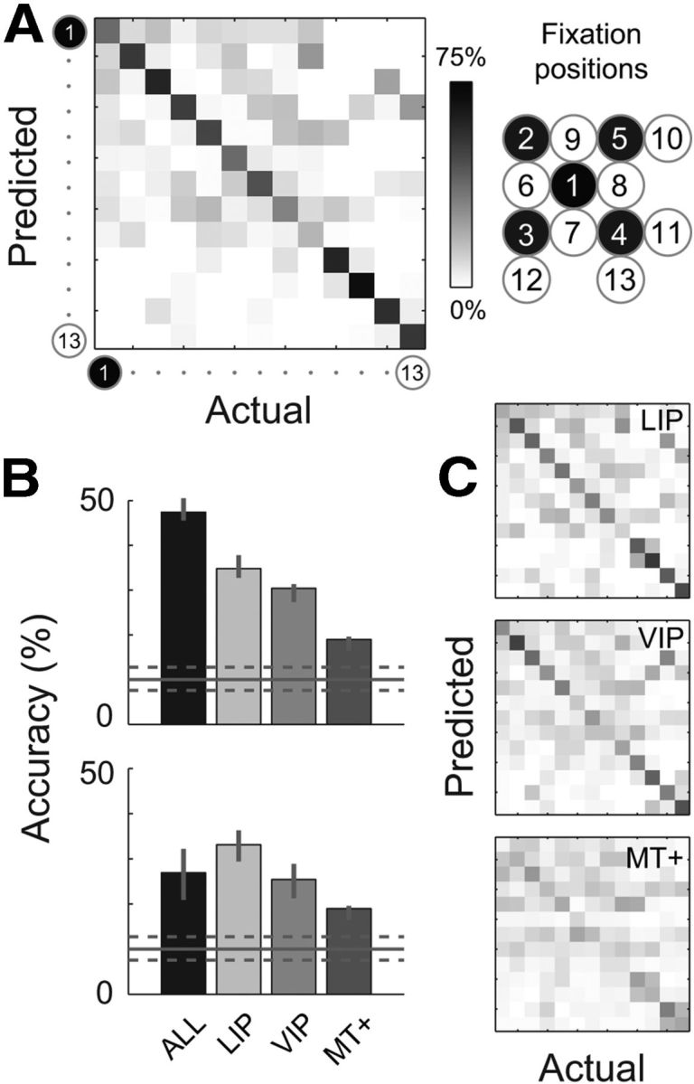
Performance of a BC algorithm that estimated eye position from neural population responses. The classifier used instantaneous spike counts (a single 100 ms sample for each neuron) from individual trials to predict which of the 13 candidate fixation positions corresponded to the current eye position. A, Performance when all the recorded neurons were used for classification, regardless of cortical area (N = 179). The confusion matrix shows the distribution of predicted eye positions for each of the 13 positions. (The ordering of fixation positions was assigned arbitrarily to the spatial arrangement shown on the right; see also Fig. 1). The density of predictions along the negative diagonal indicates good overall accuracy for the 13-alternative task (47.39% correct). B, Mean accuracy across all fixation positions (i.e., mean percentage along the diagonal of the confusion matrix), plotted separately for classifiers that estimated on the basis of all neurons in our sample (“ALL”) or on each cortical area separately. The upper plot shows accuracy for the full sample size in each case (N = 60, 69, and 50, and 179 for areas LIP, VIP, MT+, and ALL, respectively). The lower plot shows accuracy for populations of a fixed size across cortical areas (N = 50; see Results). Error bars indicate 95% confidence intervals, obtained by repeating the entire analysis on 100 bootstrap samples of neurons from each area. The horizontal solid and dashed lines in each plot indicate the mean and confidence intervals for 100 null empirical datasets (each with randomly shuffled eye-position labels). Accuracy values above or below the dashed lines are therefore significantly different from chance. C, Confusion matrices for the individual cortical areas (unequal population sizes), plotted in the same format as in A.

There was indeed a good density of correct predictions, with an overall accuracy of 47.39% (i.e., the average of the percentages along the diagonal). This level of performance is nearly five times that expected if one used only the prior probabilities (10%; see Materials and Methods). The statistical significance of this result was confirmed by comparing the observed accuracy measure with those of 100 empirical null datasets (obtained by shuffling the eye-position labels; Fig. 6B). Importantly, this result cannot be the result of overfitting because the classifier was trained and tested on statistically independent trial sets.

Figure 6, B and C, shows the accuracy and confusion matrices for the separate decoding of LIP, VIP, and MT+ neurons, ordered by performance. LIP (N = 60) and VIP (N = 69) provided reliable information about eye position, with overall accuracies of 34.81 and 30.40%, respectively. MT+ (N = 50) achieved only 18.96% correct, which was significantly better than chance but poor in absolute terms and relative to LIP and VIP. In making such a comparison, however, it is important to note that the number of neurons available to the classifier for area MT+ was less than those of the other areas. This factor alone is expected to affect performance, because the more neurons that are available to a decoder the more it can accumulate signal in the data and average out the effects of noise. To compare cortical regions on fair ground, we selected 100 random subsets of 50 neurons from each area to compare with the 50 MT+ neurons. This additional analysis yielded the same pattern of results across areas as that of the full dataset (Fig. 6B). To assess these differences statistically, we ran permutation tests (each consisting of 500 resampled, null-difference datasets) for all three possible comparisons between areas. These tests confirmed that that for matched population sizes, LIP and VIP each performed significantly better than area MT+ (both p < 0.001), while areas LIP and VIP did not differ significantly from each other (p = 0.348).

Maximum-likelihood estimation

The BC approach provided a useful first insight into the fidelity of eye-position signals in each of the studied cortical regions. A more informative approach, however, is to transform neural responses into explicit, metric estimates of eye azimuth and elevation. This method has the advantage that it mirrors more closely the estimation problem faced by the brain during everyday behavior, in which the eye can adopt one of an essentially infinite number of positions over a wide oculomotor range. Moreover, it yields intuitive measures of both the accuracy (constant error) and precision (variable error) of the cortical representation for different regions of oculomotor space.

The BC method relied on two key ingredients for classification: the prior probability of each of the 13 fixation positions in the task, and learned knowledge of the spike-count distributions associated with these positions for each neuron. MLE, in contrast, discards the prior and extends the spike-count probability model to a continuous description across a wide range of oculomotor space (i.e., it incorporates a parametric description of each neuron's pEPF). Given a population response, the ML estimator uses the pEPFs to determine which point in oculomotor space is most likely to be the true current eye position.

As for the BC method, we introduce the MLE approach by first examining its performance when applied to all of the neurons in our dataset, pooled across cortical areas. Figure 7A shows the median estimated eye position for each of the initial and target fixation positions. The decoded eye position closely approximated the true position across all of the fixation positions, with a mean constant error of 2.71° (SE = 0.25°). A closer look at the data shows that these small errors were not random in direction, but rather tended to point toward the primary (i.e., straight ahead) oculomotor position (Fig. 7B). The gain of the decoded signals (i.e., decoded eye eccentricity divided by actual eye eccentricity) was 0.87 on average (SE = 0.02) across the 13 fixation positions. Together, these results point to an accurate, though slightly compressed, representation of eye position in cortex.

Figure 7.

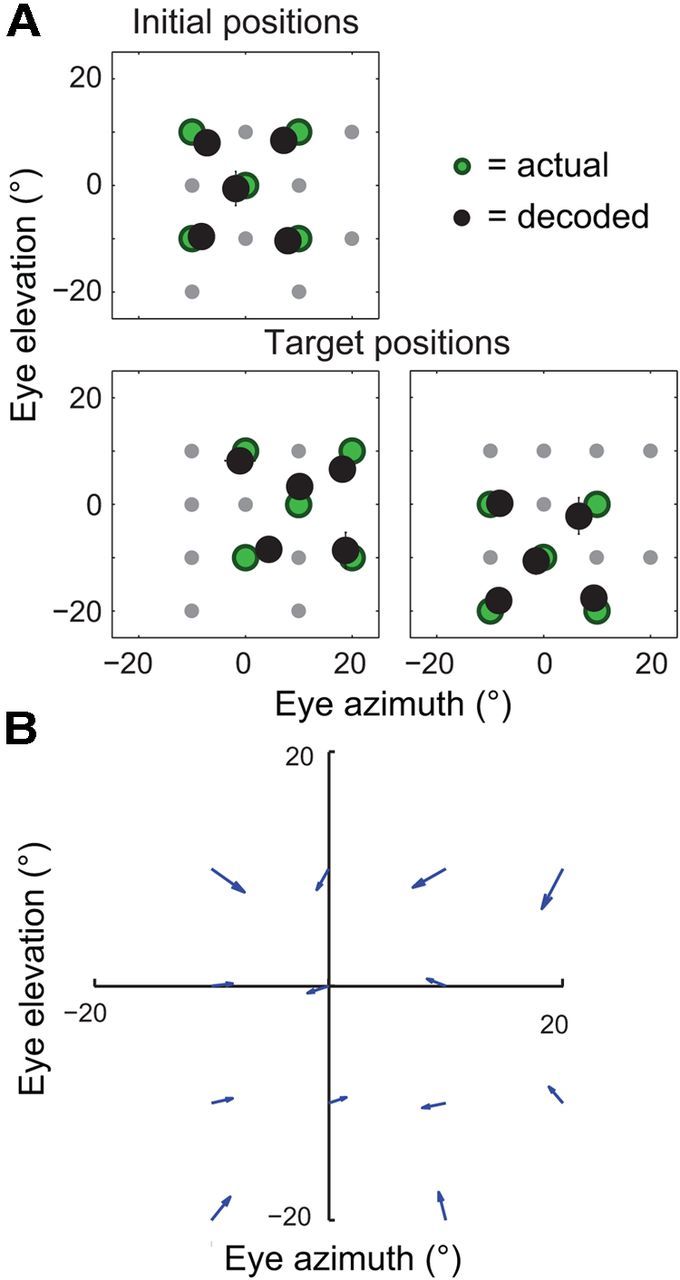
The accuracy of eye-position signals in the dorsal visual system, as evaluated by maximum-likelihood decoding of 179 neurons from areas LIP, VIP, and MT+. A, Median decoded eye position (black circles) for each of the initial (top) and target (bottom) fixation positions (each point is the average median value across cross-validation test sets, ±1 SE [i.e., SD across test sets]; most error bars are smaller than their associated symbols). The true fixation positions are also shown (green circles). The decoded eye positions closely matched the true eye position in every case, pointing to an accurate representation of eye position in these visual areas. B, The constant errors from A replotted as a vector plot to highlight the centripetal pattern of bias across oculomotor space (the data for the two non-unique fixation positions were averaged). Each arrow points from a true fixation position to the associated average decoded position. The arrows tend to point toward the straight-ahead position (0°, 0°), consistent with a spatially compressed cortical representation of eye eccentricity.

From trial to trial (and time point to time point), however, there was considerable variability in the individual estimates. Figure 8 shows the distributions of decoded positions for the five initial fixation positions. The eccentric fixation positions were associated with relatively narrow distributions, with an average dispersion, defined as the median absolute deviation, of 5.58° (SE = 0.22°). In contrast, the central fixation position was represented imprecisely, with a dispersion value about 50% higher than the eccentric positions (8.26°). This result points to an inhomogeneity in the precision of eye-position signals across oculomotor space. We will explore this effect further in a later section.

Figure 8.

Trial-to-trial (and moment-to-moment) dispersion of decoder estimates across all 100 ms samples during fixation. Each plot shows the distribution of decoder estimates associated with an initial fixation position, arranged spatially to match the task layout. Dispersion was small for the eccentric fixation positions relative to that of the central fixation position.

The same analyses were for performed for the separate decoding of LIP, VIP, and MT+ neurons (Fig. 9). For areas LIP and VIP, the accuracy of the ML decoder was comparable to that of the pooled-area dataset reported above (cf. Fig. 7). In contrast, area MT+ was associated with large, centripetal biases. The more striking difference between the performance of the individual areas and the pooled dataset was a large increase in the variability of individual estimates across samples (Fig. 10). LIP, VIP, and MT+ were associated with dispersion values of 8.45° (SE = 0.37°), 10.07° (SE = 0.54°), and 13.15° (SE = 0.50°), respectively, on average across the 13 fixation positions. These values are large enough that one might question the usefulness of such signals for spatial perception and behavior. Such a perspective, however, ignores the fact that the precision of a population code depends critically on the number of neurons. The sample sizes used here (N = 50–69) are many orders of magnitude smaller than those available in these cortical regions in natura.

Figure 9.

The accuracy of eye-position signals, plotted separately for areas LIP (N = 60), VIP (N = 69) and MT+ (N = 50). The plots are in the same format as Figure 7A.

Figure 10.

The precision of eye-position signals, plotted separately for areas LIP (N = 60), VIP (N = 69), and MT+ (N = 50). The plots are in the same format as Figure 8.

To examine the effect of population size on precision, we resampled populations of smaller sizes (with replacement) from the total sample of neurons in each area and performed MLE on each bootstrap sample. Figure 11 shows the observed relationship between the population size and the dispersion of ML estimates for each cortical area, plotted in log-log coordinates. In each case, the dispersion decreased approximately linearly with (log) population size, with slope values of −0.52, −0.46, and −0.40 for areas LIP, VIP, and MT+, respectively. Precision therefore improved approximately in proportion to the square root of the population size (i.e., a slope of −0.50 in log-log coordinates), as expected if each neuron acted as an independent estimator of eye position corrupted by Gaussian noise.

Figure 11.

Dispersion of maximum-likelihood estimates as a function of population size, plotted separately for each cortical area in log-log coordinates. The analyses that generated the results shown in Figure 10 were repeated for each of 100 bootstrapped datasets at each population size. Smaller population sizes were simulated by randomly selecting (with replacement) n out of N neurons, where n is the population size and N is the total number of neurons available in our sample for a given area. Each data point is the mean (log) dispersion value (across all fixation positions) averaged across all 100 resampled datasets, ±1 SE (i.e., the SD across the 100 values). Slope values of the least-squares regression lines (dashed) were close to −0.5 for each area, indicating that the dispersion of decoder estimates decreased approximately in proportion to the square root of the population size.

Using the fitted linear relations, we can estimate the number of neurons that would be required to achieve a criterion level of precision, assuming statistical independence among neurons. Adopting a criterion dispersion of 3°, we estimated that ∼457, 950, and 2258 neurons would be required in areas LIP, VIP, and MT+, respectively. Although these projections should be interpreted with caution, because they ignore the potential influence of noise correlations among neurons on population codes, their modest scale demonstrates that a reliable representation of eye position is likely to exist in these cortical areas.

MLE: precision depends on eye eccentricity

As noted earlier, the precision of decoding was not uniform across the 13 fixation positions spanned by the task; rather, eccentric fixation positions were associated with higher precision than the central eye position. This effect was evident in the histograms of decoder estimates for the initial fixation positions (Figs. 8, 10), but is examined directly for all fixation positions and for each cortical area in Figure 12A. The data are plotted as precision (i.e., the inverse of dispersion) heat maps, and normalized with respect to the precision of the central fixation position to facilitate a comparison across areas. In each case, there was a strong and statistically reliable effect of fixation eccentricity, with an ∼50–100% increase in precision from the central to most peripheral fixation positions. This effect was well described by a quadratic relation between fixation eccentricity and decoder precision (Fig. 12B).

Figure 12.

The representation of eye position is more precise for eccentric fixation positions than for the primary (central) position. A, Each heat map shows the pattern of precision (i.e., the inverse of dispersion) across the 13 unique fixation positions spanned by the animal's task. The data for each cortical area are normalized relative to the observed precision for the central fixation position, such that a value of 100% indicates a doubling of precision relative to that of the primary oculomotor position. The data have been interpolated (using natural neighbor interpolation) to highlight the pattern across oculomotor space. B, Mean non-normalized precision values for each of the 13 fixation positions, plotted as a function of their eccentricity (black circles). Error bars indicate the SEM (i.e., the SD of precision measures across 100 bootstrap samples; most error bars are smaller than their associated symbols). Average precision values at each eccentricity are also plotted (magenta circles). Regression analyses confirmed a significant quadratic effect of eccentricity on precision for each of the cortical areas (magenta lines; all F > 11.75, all p < 0.01).

To understand the origin of this precision effect, it is necessary to consider the factors that contribute to variability of ML estimates in this context. Ultimately, of course, the variability reflects the stochastic fluctuations of neural spiking, and so we might expect that the inhomogeneous pattern of decoder precision reflects a similar anisotropy in the variability of spike rates across oculomotor space. This simple hypothesis, however, overlooks the fact that in addition to spike-count variability, the shape of neural EPFs has direct consequences for the “precision” (technically, the entropy) of a neuron's eye-position PDF on a given trial. All else being equal, regions of oculomotor space in which the EPF is steep will be encoded with higher precision (Fig. 13A). These two factors, spike-count variability and the local gradients of neural EPFs, jointly determine the precision of the decoder. Therefore, a second hypothesis is that the eccentricity effect arises from differences in the local gradient of EPFs for central and peripheral fixation positions, or in other words, from the nonlinear aspects of neural EPFs.

Figure 13.

The dependence of decoder precision on fixation eccentricity reflects the nonlinear aspects of neural EPFs. A, Two possible explanations for a difference in precision between two regions of oculomotor space. In these simulated one-dimensional scenarios, a maximum-likelihood decoder was used to estimate eye position from the spike counts of a single neuron at two different eye positions (x₁ and x₂) using knowledge of its EPF (blue lines). In both scenarios, the decoder generated imprecise estimates for position x₁ and precise estimates for x₂, as indicated by the wide (black) and narrow (gray) distributions below each plot. In the “Unequal rate variance” scenario, the difference in precision reflects different levels of noise on the firing rates at the two eye positions, as indicated by the black and gray distributions on the rate (y) axis. In the “Unequal EPF gradient” scenario, the two fixation positions were associated with equal neural noise but had different local gradients on the EPF due to a quadratic nonlinearity. Nevertheless, the two scenarios generated almost identical decoding outcomes. B, A test of the two possible explanations for the eccentricity effect on precision. Two quantities were computed for each neuron in our sample at each of the 13 unique fixation positions. The first was the variance of firing rates across trials. The second was the local gradient of the fitted 2D EPF regression function. The median values of these two measures across neurons are plotted against the corresponding precision measurements for each fixation position (from Fig. 12B), separately for the pooled-area analysis and each cortical area. Precision correlated strongly with the local EPF gradient and not with rate variance, suggesting that the eccentricity effect arises from the nonlinear aspects of neural EPFs. *p < 0.05; **p < 0.001.

To determine which of these explanations could better account for the eccentricity effect, we plotted the precision values for each of the 13 fixation positions against both the associated median firing rate variance and the median local gradient of the EPFs across the population (Fig. 13B). The precision measurements correlated poorly and nonsignificantly with spike-rate variance for the pooled-area analysis, and for areas VIP and MT+. In contrast, strong and consistent correlations were observed between the precision measurements and the local EPF gradient in every case, suggesting that this variable provides a good explanation for the pattern of decoder precision.

Comparison with human behavior

In Figure 7 we observed a compressed neural representation of eye position in the dorsal visual system, such that the decoded positions were biased toward the primary oculomotor position. If cortical EPFs are used to localize visual objects in the environment, as has been suggested (Andersen et al., 1985; Zipser and Andersen, 1988), then these systematic errors might be observable in human behavior. Such effects could be expected in tasks that rely on knowledge of eye position, such as pointing toward a visual target without sensory feedback.

In Figure 14, we compare the localization errors that would be predicted on the basis of our electrophysiological measurements with data from two such studies of human performance (Morgan, 1978; Lewald and Ehrenstein, 2000). In both studies, the task was to point in the direction of a foveated visual target at a range of different azimuthal eye positions (elevational eye positions and errors were not examined). Because the experiments were performed in complete darkness, and with the head straight ahead, accurate localization relied on internal knowledge of eye position. The predictions from the neural data (black dots and line) were generally consistent with the human behavioral data (red and green dots) and even matched the data of the Lewald and Ehrenstein study in a quantitative manner (97% performance variance explained).

Figure 14.

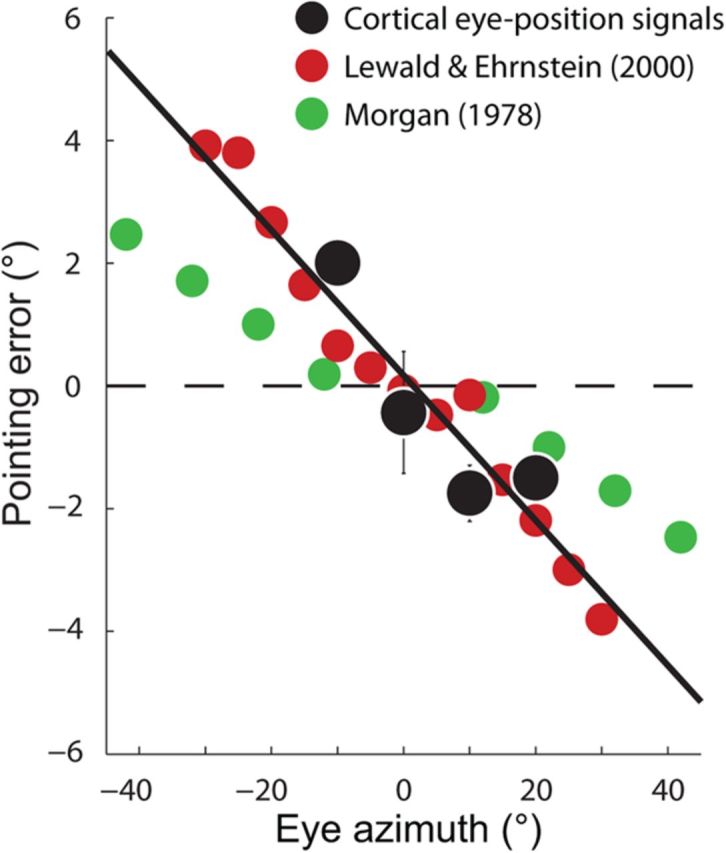
The cortical (mis)representation of eye position predicts localization errors that match human performance. Pointing to a foveated visual target in darkness (with the head aligned with the body) requires knowledge of the current eye position. Accordingly, the pattern of constant error observed in Figure 7 predicts that pointing movements to eccentric targets should be biased toward the straight-ahead position. Behavioral studies of this kind have been performed in human observers for targets at different positions along the horizontal meridian. The pointing errors from two such studies (red and green dots) are reproduced in the figure, plotted as a function of target (eye) eccentricity. Positive and negative values on the ordinate indicate rightward and leftward mislocalization errors, respectively. The results from both studies are consistent with a compressed internal representation of eye position in the human observers. To compare these data with the macaque physiology, we averaged and plotted the azimuthal error values from Figure 7 at each of the four unique azimuthal eccentricities (black dots). Error bars indicate ±1 SE. A regression line fitted to the neural data (black line) summarized the centripetal biases in the cortical representation of eye position and provided a good match to the human behavioral data.

Discussion

This study examined eye-position signals in four areas of the dorsal visual system (LIP, VIP, MT, and MST). We used population-decoding approaches to take into account not only changes in the signal carried by neurons (i.e., mean firing rate) across different eye positions, but also the associated noise (i.e., spike-count variability for constant eye positions). The combined influence of these variables determined both the accuracy (i.e., constant error) and the precision (i.e., variable error) of population codes for eye position over short timescales. In turn, these performance measures allowed an assessment of whether cortical eye-position signals could be useful for real-time coding of egocentric spatial positions.

The accuracy of eye-position signals

Taken as a whole, our analysis shows that cortical EPFs provided a highly accurate representation of eye position during fixation: constant error of MLEs was within a few degrees of visual angle across the extent of oculomotor space considered. At a finer scale, we found that these errors were not random in direction but rather were biased toward the primary position. This implies that cortical eye-position signals underestimate the eccentricity of gaze.

If the decoded signals were used to localize visual objects, perceived positions would be compressed toward the head midline (or body midline; Brotchie et al., 1995). Whether such a bias would be observable in behavior is unclear. In principle, the compression could be annulled during downstream computations, resulting in unbiased behavior (this is equivalent to adopting a different decoding rule or different parametric expression for EPFs than those used here). Even if not corrected, however, the misrepresentation may be masked during everyday behavior because of the availability of other spatial cues and strategies (e.g., visual guidance). In that case, there would be no error signal to drive calibratory processes (Redding and Wallace, 1996) and the misrepresentations might be detectable in the laboratory.

Investigators have probed eye-position signals using a variety of behavioral tasks. For example, Lewald and Ehrenstein (2000) had human observers localize visual targets at a range of azimuthal positions using a hand-held pointer. Importantly, the targets were foveated in darkness and with the head directed straight ahead, such that accurate localization relied on knowledge of eye position. These authors observed a centripetal bias in performance that was proportional to eye eccentricity, suggesting that subjects used a compressed representation of eye position. As shown here, this misrepresentation was consistent with that of cortical EPFs (Fig. 14). Similar compression effects have been observed across a number of behavioral studies (Hill, 1972; Morgan, 1978; Enright, 1995), though with different magnitudes and in some instances, no compression at all (Bock, 1986; Rossetti et al., 1994).

In a different kind of study, James et al. (2001) had observers judge the slant of a cube face seen at different azimuthal positions–a task that relies on knowledge of eye position but does not require a spatially directed response (thus minimizing motor-related biases). Consistent with the localization studies, they found that subjects undercompensated for the change in eye position, as if the brain used a compressed representation of eye position for the perception of object slant (Ebenholtz and Paap, 1973).

This consistency across studies, and their qualitative match with the macaque physiology reported here, supports the notion that EPFs play a direct role in the spatial computations for action planning and perception (Zipser and Andersen, 1988; Pouget and Sejnowski, 1997; Salinas and Sejnowski, 2001). This is contrary to the view that they serve only a slow, calibratory purpose (Wang et al., 2007; Xu et al., 2012). In addition, we recently showed that the dynamics of EPFs provide a good account of well known localization errors that occur for briefly flashed targets around the time of saccades (Morris et al., 2012). In that study, we showed that the cortical representation of eye position is updated predictively but with slow dynamics, such that it represents a temporally smoothed version of the eye movement. This damped representation matched a long-standing hypothetical eye-position signal that had been estimated from psychophysical measurements (Honda, 1990, 1991; Dassonville et al., 1992).

Finally, in anticipation of potential confusion, we note that the compression effect reported here is distinct from the psychophysical “compression of visual space” that is found around the time of saccades (Ross et al., 2001). The latter phenomenon is characterized by a transient mislocalization of visual probes toward the location of a saccade target in eye-centered coordinates, not toward the head midline or body midline as would be predicted on the basis of the current findings. This study therefore does not directly bear on the issue of perisaccadic perceptual compression. Previously, however, we showed that the representation of a target's position on the retina is distorted at the time of saccades in a manner that could account for the compression of visual space (Krekelberg et al., 2003).

The precision of cortical eye-position signals

Precision, in this context, refers to variability of population codes for eye position from one moment to the next, and thus is a key determinant of the usefulness of such signals for real-time spatial computations. We quantified precision as the dispersion of population estimates for constant eye positions, regardless of the associated accuracy. Dispersion values were generally large, around 5° on average for the decoding of eye position from our total sample, and higher still for the separate decoding of neurons in LIP, VIP, and MT+. Superficially, these values would imply that cortical eye-position signals would be too unreliable for spatial coding on behaviorally relevant timescales. Population codes, however, typically become more reliable as the number of neurons increases, and the brain no doubt calls on much larger pools of neurons in natura than those sampled here (Boussaoud and Bremmer, 1999; Averbeck et al., 2006). Indeed, population-size analyses suggested that a highly precise representation of eye position should be available in these dorsal visual areas. Without knowledge of the correlational structure of the spike-count variability, however, it is not possible to form a definitive conclusion in this regard (Averbeck et al., 2006). Future experiments that record from multiple neurons simultaneously could address this issue.

Another key finding was that precision depended strongly on the eccentricity of fixation. The outermost fixation positions (eccentricity = 22.5°) were decoded with approximately twice the precision of the central position. This inhomogeneity was evident in each of the cortical areas we examined and was attributable to the nonlinear (i.e., quadratic) aspects of EPFs. Specifically, correlation analysis suggested that the increase in precision for peripheral positions reflected a tendency toward steeper local EPF gradients (and hence, enhanced discriminability of eye positions), and not decreased variability of neuronal spiking. This implies that nonlinearities in cortical EPFs have important consequences for the representation of eye position.

The effects of eccentricity on precision predict a specific pattern of performance on tasks that rely on eye-position signals. Few studies have attempted to isolate the eye-position contribution to variability in behavioral responses, and the results are inconsistent. For example, Enright (1995) observed an increase in the precision of pointing movements during eccentric fixation (approximately 25%, calculated from Enright, 1995, his Table 1), consistent with the results of the current study. Rossetti et al. (1994) and Blohm and Crawford (2007), in contrast, found a decrease in pointing precision with increasing eccentricity of eye position. These discrepancies across studies suggest that it may be difficult to isolate the contribution of noisy eye-position representations to behavioral measures. This is perhaps not surprising given that variable error in such measurements reflects the cumulative noise across all stages of the sensorimotor pathway, of which eye-position signals make up only a fraction. Moreover, in such studies, it is impossible to vary eye position independently of other noise-producing spatial variables (e.g., position of the target on the retina, or, position of the target relative to the body). Nevertheless, by modeling the full sensorimotor transformation from eye to hand, Blohm and Crawford (2007) showed that the behavioral variability in their study was best explained by increased noise in eye-position signals during eccentric fixation. This pattern is opposite to that of the current study. Thus, the link between our physiological findings and measurements of behavioral variability requires further investigation.

Signal fidelity across cortical areas

LIP and VIP population codes carried more accurate and precise representations of eye position relative to those in MT+ (MT and MST combined), even when matched for sample size. The cause of these area differences is unknown. One possibility is that they reflect the different functional roles attributed to these areas: LIP and VIP are more directly implicated in movement planning and/or multisensory integration (Colby and Goldberg, 1999; Andersen and Buneo, 2002; Bremmer, 2005) than are areas MT and (to a lesser extent) MST–roles for which eye-position information is crucial. Alternatively, eye-position signals in area MT+ might depend more strongly on the presence of visual stimulation (and the associated increase in firing rates).

Conclusion

Cortical EPFs provide a representation of eye position that is sufficiently accurate and precise on short timescales to support their purported role in on-line spatial computation. The small mismatch between the actual eye position and that represented in the dorsal-visual system can account for known spatial biases in human perception and action.

References

- Andersen RA, Buneo CA. Intentional maps in posterior parietal cortex. Annu Rev Neurosci. 2002;25:189–220. doi: 10.1146/annurev.neuro.25.112701.142922. [DOI] [PubMed] [Google Scholar]
- Andersen RA, Mountcastle VB. The influence of the angle of gaze upon the excitability of the light-sensitive neurons of the posterior parietal cortex. J Neurosci. 1983;3:532–548. doi: 10.1523/JNEUROSCI.03-03-00532.1983. [DOI] [PMC free article] [PubMed] [Google Scholar]
- Andersen RA, Zipser D. The role of the posterior parietal cortex in coordinate transformations for visual-motor integration. Can J Physiol Pharmacol. 1988;66:488–501. doi: 10.1139/y88-078. [DOI] [PubMed] [Google Scholar]
- Andersen RA, Bracewell RM, Barash S, Gnadt JW, Fogassi L. Eye-position effects on visual, memory, and saccade-related activity in areas LIP and 7a of macaque. J Neurosci. 1990;10:1176–1196. doi: 10.1523/JNEUROSCI.10-04-01176.1990. [DOI] [PMC free article] [PubMed] [Google Scholar]
- Andersen RA, Essick GK, Siegel RM. Encoding of spatial location by posterior parietal neurons. Science. 1985;230:456–458. doi: 10.1126/science.4048942. [DOI] [PubMed] [Google Scholar]
- Averbeck BB, Latham PE, Pouget A. Neural correlations, population coding and computation. Nat Rev Neurosci. 2006;7:358–366. doi: 10.1038/nrn1888. [DOI] [PubMed] [Google Scholar]
- Blohm G, Crawford JD. Computations for geometrically accurate visually guided reaching in 3-D space. J Vis. 2007;7(5):4.1–22. doi: 10.1167/7.5.4. [DOI] [PubMed] [Google Scholar]
- Bock O. Contribution of retinal versus extraretinal signals towards visual localization in goal-directed movements. Exp Brain Res. 1986;64:476–482. doi: 10.1007/BF00340484. [DOI] [PubMed] [Google Scholar]
- Boussaoud D, Bremmer F. Gaze effects in the cerebral cortex: reference frames for space coding and action. Exp Brain Res. 1999;128:170–180. doi: 10.1007/s002210050832. [DOI] [PubMed] [Google Scholar]
- Bremmer F. Navigation in space–the role of the macaque ventral intraparietal area. J Physiol. 2005;566:29–35. doi: 10.1113/jphysiol.2005.082552. [DOI] [PMC free article] [PubMed] [Google Scholar]
- Bremmer F, Pouget A, Hoffmann KP. Eye-position encoding in the macaque posterior parietal cortex. Eur J Neurosci. 1998;10:153–160. doi: 10.1046/j.1460-9568.1998.00010.x. [DOI] [PubMed] [Google Scholar]
- Bremmer F, Kubischik M, Hoffmann KP, Krekelberg B. Neural dynamics of saccadic suppression. J Neurosci. 2009;29:12374–12383. doi: 10.1523/JNEUROSCI.2908-09.2009. [DOI] [PMC free article] [PubMed] [Google Scholar]
- Brotchie PR, Andersen RA, Snyder LH, Goodman SJ. Head position signals used by parietal neurons to encode locations of visual stimuli. Nature. 1995;375:232–235. doi: 10.1038/375232a0. [DOI] [PubMed] [Google Scholar]
- Colby CL, Goldberg ME. Space and attention in parietal cortex. Annu Rev Neurosci. 1999;22:319–349. doi: 10.1146/annurev.neuro.22.1.319. [DOI] [PubMed] [Google Scholar]
- Dassonville P, Schlag J, Schlag-Rey M. Oculomotor localization relies on a damped representation of saccadic eye displacement in human and nonhuman primates. Vis Neurosci. 1992;9:261–269. doi: 10.1017/S0952523800010671. [DOI] [PubMed] [Google Scholar]
- Ebenholtz SM, Paap KR. The constancy of object orientation: compensation for ocular rotation. Percep Psychophys. 1973;14:458–470. doi: 10.3758/BF03211184. [DOI] [Google Scholar]
- Enright JT. The non-visual impact of eye orientation on eye-hand coordination. Vision Res. 1995;35:1611–1618. doi: 10.1016/0042-6989(94)00260-S. [DOI] [PubMed] [Google Scholar]
- Graf AB, Kohn A, Jazayeri M, Movshon JA. Decoding the activity of neuronal populations in macaque primary visual cortex. Nat Neurosci. 2011;14:239–245. doi: 10.1038/nn.2733. [DOI] [PMC free article] [PubMed] [Google Scholar]
- Hill AL. direction constancy. Percep Psychophys. 1972;11:175–178. doi: 10.3758/BF03210370. [DOI] [Google Scholar]
- Honda H. Eye movements to a visual stimulus flashed before, during, or after a saccade. In: Jeannerod M, editor. Attention and performance. Hillsdale, NJ: Lawrence Erlbaum; 1990. pp. 567–582. [Google Scholar]
- Honda H. The time courses of visual mislocalization and of extraretinal eye-position signals at the time of vertical saccades. Vision Res. 1991;31:1915–1921. doi: 10.1016/0042-6989(91)90186-9. [DOI] [PubMed] [Google Scholar]
- James FM, Whitehead S, Humphrey GK, Banks MS, Vilis T. Eye-position sense contributes to the judgement of slant. Vision Res. 2001;41:3447–3454. doi: 10.1016/S0042-6989(01)00118-3. [DOI] [PubMed] [Google Scholar]
- Kaplan DM, Snyder LH. The need for speed: eye-position signal dynamics in the parietal cortex. Neuron. 2012;76:1048–1051. doi: 10.1016/j.neuron.2012.12.005. [DOI] [PubMed] [Google Scholar]
- Kass RE, Ventura V, Brown EN. Statistical issues in the analysis of neuronal data. J Neurophysiol. 2005;94:8–25. doi: 10.1152/jn.00648.2004. [DOI] [PubMed] [Google Scholar]
- Knill DC, Pouget A. The Bayesian brain: the role of uncertainty in neural coding and computation. Trends Neurosci. 2004;27:712–719. doi: 10.1016/j.tins.2004.10.007. [DOI] [PubMed] [Google Scholar]
- Krekelberg B, Kubischik M, Hoffmann KP, Bremmer F. Neural correlates of visual localization and perisaccadic mislocalization. Neuron. 2003;37:537–545. doi: 10.1016/S0896-6273(03)00003-5. [DOI] [PubMed] [Google Scholar]
- Lewald J, Ehrenstein WH. Visual and proprioceptive shifts in perceived egocentric direction induced by eye-position. Vision Res. 2000;40:539–547. doi: 10.1016/S0042-6989(99)00197-2. [DOI] [PubMed] [Google Scholar]
- Ma WJ, Beck JM, Latham PE, Pouget A. Bayesian inference with probabilistic population codes. Nat Neurosci. 2006;9:1432–1438. doi: 10.1038/nn1790. [DOI] [PubMed] [Google Scholar]
- Macmillan NA, Creelman CD. Detection theory: a user's guide. Ed 2. Mahwah, N.J.: Lawrence Erlbaum; 2005. [Google Scholar]
- Morgan CL. Constancy of egocentric visual direction. Percept Psychophys. 1978;23:61–68. doi: 10.3758/BF03214296. [DOI] [PubMed] [Google Scholar]
- Morris AP, Kubischik M, Hoffmann KP, Krekelberg B, Bremmer F. Dynamics of eye-position signals in the dorsal visual system. Curr Biol. 2012;22:173–179. doi: 10.1016/j.cub.2011.12.032. [DOI] [PMC free article] [PubMed] [Google Scholar]
- Pouget A, Sejnowski TJ. Spatial transformations in the parietal cortex using basis functions. J Cogn Neurosci. 1997;9:222–237. doi: 10.1162/jocn.1997.9.2.222. [DOI] [PubMed] [Google Scholar]
- Redding GM, Wallace B. Adaptive spatial alignment and strategic perceptual-motor control. J Exp Psychol Hum Percept Perform. 1996;22:379–394. doi: 10.1037/0096-1523.22.2.379. [DOI] [PubMed] [Google Scholar]
- Ross J, Morrone MC, Goldberg ME, Burr DC. Changes in visual perception at the time of saccades. Trends Neurosci. 2001;24:113–121. doi: 10.1016/S0166-2236(00)01685-4. [DOI] [PubMed] [Google Scholar]
- Rossetti Y, Tadary B, Prablanc C. Optimal contributions of head and eye-positions to spatial accuracy in man tested by visually directed pointing. Exp Brain Res. 1994;97:487–496. doi: 10.1007/BF00241543. [DOI] [PubMed] [Google Scholar]
- Salinas E, Abbott LF. Vector reconstruction from firing rates. J Comput Neurosci. 1994;1:89–107. doi: 10.1007/BF00962720. [DOI] [PubMed] [Google Scholar]
- Salinas E, Sejnowski TJ. Gain modulation in the central nervous system: where behavior, neurophysiology, and computation meet. Neuroscientist. 2001;7:430–440. doi: 10.1177/107385840100700512. [DOI] [PMC free article] [PubMed] [Google Scholar]
- Tolhurst DJ, Movshon JA, Dean AF. The statistical reliability of signals in single neurons in cat and monkey visual cortex. Vision Res. 1983;23:775–785. doi: 10.1016/0042-6989(83)90200-6. [DOI] [PubMed] [Google Scholar]
- Wang X, Zhang M, Cohen IS, Goldberg ME. The proprioceptive representation of eye-position in monkey primary somatosensory cortex. Nat Neurosci. 2007;10:640–646. doi: 10.1038/nn1878. [DOI] [PubMed] [Google Scholar]
- Xu BY, Karachi C, Goldberg ME. The postsaccadic unreliability of gain fields renders it unlikely that the motor system can use them to calculate target position in space. Neuron. 2012;76:1201–1209. doi: 10.1016/j.neuron.2012.10.034. [DOI] [PMC free article] [PubMed] [Google Scholar]
- Zipser D, Andersen RA. A back-propagation programmed network that simulates response properties of a subset of posterior parietal neurons. Nature. 1988;331:679–684. doi: 10.1038/331679a0. [DOI] [PubMed] [Google Scholar]