

Abstract
The femoral neck-shaft angle (NSA) varies among modern humans but measurement problems and sampling limitations have precluded the identification of factors contributing to its variation at the population level. Potential sources of variation include sex, age, side (left or right), regional differences in body shape due to climatic adaptation, and the effects of habitual activity patterns (e.g. mobile and sedentary lifestyles and foraging, agricultural, and urban economies). In this study we addressed these issues, using consistent methods to assemble a global NSA database comprising over 8000 femora representing 100 human groups. Results from the analyses show an average NSA for modern humans of 127° (markedly lower than the accepted value of 135°); there is no sex difference, no age-related change in adults, but possibly a small lateral difference which could be due to right leg dominance. Climatic trends consistent with principles based on Bergmann's rule are evident at the global and continental levels, with the NSA varying in relation to other body shape indices: median NSA, for instance, is higher in warmer regions, notably in the Pacific (130°), whereas lower values (associated with a more stocky body build) are found in regions where ancestral populations were exposed to colder conditions, in Europe (126°) and the Americas (125°). There is a modest trend towards increasing NSA with the economic transitions from forager to agricultural and urban lifestyles and, to a lesser extent, from a mobile to a sedentary existence. However, the main trend associated with these transitions is a progressive narrowing in the range of variation in the NSA, which may be attributable to thermal insulation provided by improved cultural buffering from climate, particularly clothing.
Keywords: Bergmann's rule, climate, clothing, femur, leg dominance, neck-shaft angle
Introduction
The angle of the femoral neck relative to the shaft (the neck-shaft angle, NSA) varies widely among modern humans and earlier hominins, even within small population samples. Adult values for modern humans generally fall within a range between 120 and 140°, although values of < 120° and > 140° are not uncommon (known as coxa varus and coxa valgus, respectively). However, reliable data on regional trends in average NSA among modern human groups are limited, due in part to measurement issues (see Bonneau et al. 2012). Furthermore, there is ongoing debate as to whether any such regional trends may reflect climatic adaptation (in relation to body shape) or habitual activity patterns – as a reflection, for instance, of forager, agricultural or urban lifestyles. Among earlier hominins, the lower NSA of Neanderthals has been interpreted as an outcome of a more mobile and physically demanding lifestyle (Trinkaus, 1993) and, alternatively, as a corollary of their more stocky, cold-adapted body build (Weaver, 2003). At the individual level, asymmetry between left and right NSA is sometimes marked, but no consistent lateral difference at the population level has been reported to date. The NSA does change during early development, being higher in juveniles and declining during childhood, usually reaching adult values by adolescence, after which it remains stable, although there may be a minor further decline with advancing age (e.g. 60 years and over). Whether a sex difference exists is open to question: the limited evidence available in physical anthropology indicates that sexual differences are minor and inconsistent (Anderson & Trinkaus, 1998) but anatomy textbooks often state that the NSA is lower in females (e.g. Standring, 2008).
The medical significance of the femoral NSA relates primarily to its possible role in the differing vulnerability of various groups to osteoarthritis at the hip joint and the risk of femoral neck fracture, which causes considerably disability among the elderly and necessitates expensive hip replacement surgery. For instance, a higher NSA among American black women compared with white women was claimed to be a contributing factor in their lower incidence of hip fracture (Walensky & O'Brien, 1968). More recent studies, however, report equivocal findings with regard to the NSA and suggest instead that osteoporosis is the main factor, with reduced bone mineral density among post-menopausal women leading to a greater susceptibility to hip fracture (e.g. Cheng et al. 1997; Pulkkinen et al. 2006; Gnudi et al. 2007; Doherty et al. 2008).
Body shape and climate
A key aspect of biological adaptation to the thermal environment involves the relationship between body shape and heat loss (Gould, 1966; Ruff, 1994). The thermal significance of body form derives from the ratio between skin surface area and body volume, or mass: the latter relates to heat production (through metabolism), whereas the exposed skin surface plays a dominant role in dissipating body heat. These considerations will result in a lighter, more linear body build in tropical climates and a heavier, more stocky build in colder environments. The adaptive relationship between body mass and climate is known as Bergmann's rule (Bergmann, 1847); a related principle, called Allen's rule, refers to the size of body appendages, with exposed limbs becoming shorter in cooler climates (Allen, 1877). Although other adaptive strategies (e.g. a thicker fur cover in cold climates) and competing selection pressures need to be taken into account (Mayr, 1956; Schreider, 1975; Katzmarzyk & Leonard, 1998), Bergmann's rule has been shown to apply among numerous bird and mammal species (e.g. Ashton et al. 2000; Meiri & Dayan, 2003). Among fossil hominins, indices of body shape and limb proportions have been shown to correlate with thermal conditions (e.g. Ruff, 1991, 1994; Holliday & Falsetti, 1995). For Neanderthals, various body shape indices indicate a more stocky body build compared with both early and contemporary Homo sapiens, reflecting Neanderthals' morphological adaptation to colder Eurasian climates during late Pleistocene ice ages (Trinkaus, 1981). In contrast, the tall, linear build of Homo ergaster was well-adapted to open, semi-arid environments in Africa (Ruff, 1993).
Similarly, studies of modern-day humans have demonstrated that body mass and shape, head shape, and relative limb proportions correlate with thermal conditions, on a global and on a continental or regional scale (e.g. Roberts, 1978; Crognier, 1981; Houghton, 1990; Ruff, 2002; Gilligan & Bulbeck, 2007). Limb proportions have also been shown to vary with altitude, for instance between coastal and highland groups in Peru (Weinstein, 2005), while moisture (in the form of humidity and rainfall) can affect the relationship between temperature and body shape. The cooling advantage of having a higher surface/volume ratio in hot environments depends largely on evaporation of perspiration from the skin surface but this is compromised in conditions of high atmospheric moisture content, especially when coupled with reduced wind chill. These environmental conditions are found in heavily forested tropical environments, which may explain the adaptive benefit of reduced body size among Pygmy and Negrito populations inhabiting hot, humid rainforest habitats. In these circumstances, where keeping cool is the main priority, the exposed skin surface is of little use for evaporative cooling but a lower body mass means less metabolic heat production, with the net thermal result of a smaller body size being reduced heat stress (Hiernaux et al. 1975; Cavalli-Sforza, 1986).
Neck-shaft angle and body shape
Despite considerable research in recent years, it remains unclear whether the NSA varies in relation to climate due to an association with body shape. In concluding that the lower NSA of Neanderthals reflects a more physically demanding lifestyle rather than adaptation to cold, Trinkaus (1993, 1994) cited NSA data on 21 modern samples from various sources grouped into three lifestyle categories (foraging, agricultural, and urban). The NSA showed a modest increase across these groups, which was interpreted as reflecting the shift to a more sedentary lifestyle (rather than any difference in thermal conditions). A subsequent study employing samples from 30 modern groups reported a similar trend; specifically, a climatic association was discounted after finding no significant trend between four groupings (Sub-Saharan African, European/Mediterranean, East Asian and Native American) and climate as measured by latitude (Anderson & Trinkaus, 1998). In contrast to Trinkaus's interpretation, Weaver (2003) analyzed 39 anatomical markers on the hip and femur among human groups from warm and cold climates and found that the lower NSA of Neanderthals was entirely consistent with a cold-climate morphology. He suggests that this lower NSA among cold-climate groups reflected differing developmental forces on the femoral neck secondary to climate-related differences in body proportions, rather than any differences due to lifestyle or activity levels. In essence, a broader, more cold-adapted body shape increases biomechanical loading on the femoral neck during early development, resulting in a lower NSA.
Body shape and clothing
Since the last ice age (which ended some 10 000 years ago), modern humans have developed increasingly elaborate – and thermally effective – forms of cultural buffering from external environmental conditions, and a likely consequence of these behavioural adaptations and technological developments is reduced selection pressure for biological adaptations. This may become visible as reduced sensitivity of body shape to climatic variation, which should be most discernible among those human groups utilizing the more sophisticated forms of artificial insulation from thermal stresses. During the last ice age, for instance, the retention of tropical limb proportions among fully modern humans in Europe is attributable to improved cultural buffering from climate (Holliday, 1997), particularly the development of complex – tailored, multi-layered – clothing assemblages (Gilligan, 2010a).
Insofar as the NSA varies with body shape and hence with morphological adaptation to climate, greater use of clothing may be expected to result in reduced sensitivity of the NSA to climatic indices. Moreover, regular use of clothing may act as a confounding variable in assessing the possible influence of lifestyle factors on variation in the NSA because the adoption of more sedentary lifestyles and the transitions between basic economic categories (such as forager, agricultural, and urban) may themselves be associated systematically with differing levels of clothing use. For instance, foragers such as the Australian Aborigines typically wore no clothing and, prior to European settlement, their use of clothing was related almost exclusively to thermal requirements (Gilligan, 2008); the Andaman Islanders in the Bay of Bengal and the Fuegian groups in southern South America are other examples. On the other hand, the advent of agricultural practices was itself associated with the production of woven fibres for more sophisticated clothing, notably thermally efficient textile garments (Gilligan, 2007). Similarly, communities that developed a fully sedentary, urban lifestyle were likewise characterized by more effective cultural buffering, creating more sophisticated forms of artificial shelter (and, in recent decades, air conditioning) as well as routinely using complex clothing. In other words, the categories that distinguish differing levels of mobility and economic activity may also distinguish differing levels of insulation from external climatic variation, providing a thermal basis for any apparent trends in the NSA between these groups.
Measurement issues
A paucity of research on the human NSA is in part attributable to problems and uncertainties regarding methods for best determining the NSA. Anatomical aspects of the proximal femur make measurement difficult, including the lack of reliable anatomical markers and the often irregular contours of the neck itself, which can render definition of the neck axis ambiguous (Bonneau et al. 2012). Even defining the shaft axis is not always straightforward, as there is not uncommonly a degree of curvature in the shaft, most typically anterior bowing. Another practical difficulty with measurement relates to the varying amount of anterior rotation of the neck in relation to the shaft – known as anteversion of the femoral neck. This latter issue means that measuring the NSA on a standard osteometric board is not viable and it becomes especially problematical where NSA measurements are taken from radiographs, as anteversion (not readily detectable on a standard X-ray) exaggerates the NSA. Although various methods and formulæ have been proposed to mitigate or compensate for the consequent errors (e.g. Ogata & Goldsand, 1979; Trinkaus, 1993), in practice it is preferable to measure the NSA directly by hand and avoid using NSA data obtained from radiographs (Olsen et al. 2009). Nonetheless, many of the older published data on NSA – still cited in the literature – derive from radiographs (e.g. Houston & Zaleski, 1967), and even recent studies sometimes utilize radiographs (e.g. Igbigbi, 2003). Conversely, notwithstanding the problems of measurement by hand (related essentially to anatomical variability and lack of reliable anatomical markers), inter- and intra-observer errors using measurement by hand have been shown to be acceptably small – usually no more than 1–2° – in relation to differences in group means (Anderson & Trinkaus, 1998). In the present study, it was planned initially to measure the NSA using an osteometric board equipped with apparatus designed specifically for measuring angles. However, anteversion proved an insurmountable problem and a hand-held goniometer was substituted, with measurements taken on the anterior surface of the femur in a plane defined by the anterior surfaces of the neck and proximal shaft, removing any confounding effect of anteversion on the measurement (E. Trinkaus, pers. comm.).
Materials and methods
Femoral samples
Skeletal collections of modern human femora were selected on the basis of provenance and measurable NSA; the majority were complete or largely intact femora, although a substantial proportion of the remainder consisted of proximal segments with sufficient portions of the neck and shaft preserved to permit measurement of the NSA. Specimens with obvious deformity or pathology (such as Paget's disease, or remodeled neck fractures) were excluded; neither juvenile nor early adolescent bones lacking epiphyseal fusion were examined. Depending on the extent of preservation or completeness, other measures were taken: femoral head diameter (FHD), bicondylar breadth (BCB), and maximum femoral length (MFL); side (left or right) was recorded, as well as sex and age at death (where available). All measurements of the NSA were taken on the femora themselves using a hand-held 360° goniometer: this minimized the confounding effect of femoral anteversion in determining NSA and avoided the perils of pooling data from other published sources where techniques differ substantially (and, in many cases, where measurements were taken on radiographs).
Given the aim of adequately sampling the NSA from a diverse range of environmental and socioeconomic contexts, the goal to maximize total sample size was balanced by a quest for broad geographical sampling. Very small samples were sometimes included: even a single femur from a certain locality or group might be measured at one institution, as this could be added to samples from other institutions or combined with larger group or regional samples in subsequent analyses. Provenance to country of origin was also a priority in determining inclusion, as each sample needed to be linked to geographical location and hence climatic indices – the main exceptions related to specific human groups (such as Bushmen, Sami, and central African Pygmies) where associations with modern national entities were less relevant. Only specimens with well documented provenance were included; all samples were from recent (Holocene epoch) contexts and were restricted to indigenous populations to minimize the effects of colonial-era migrations (e.g. Aboriginal Australians, and Native American groups in the Americas).
A total of 8271 femora were measured. The institutions involved in the study (and the number of femora measured at each) are listed in Supporting Information Table S1. The number of groups sampled was 101, representing 80 countries, 10 territories, and 11 other groups. One of the country samples (the Cote d'Ivoire) comprised only a single femur: this was included in some of analyses as part of the global and African continental samples but was excluded from statistical analyses utilizing group means, yielding 100 groups (countries/territories/other groups). Territories are locales considered independently of the countries responsible for their administration, e.g. Canary Islands (Spain), Easter Island (Chile), Greenland (Denmark), Guadeloupe (France), Guam (USA), Marquesas Islands (France), Nicobar Islands (India), and Tahiti (France). The Russian Far East (a Russian federal district formerly known loosely as Siberia) was here considered separately from Russia, as a part of the Asian continent rather than Europe; Hawaii, a state of the USA, was considered as a separate group (being one of the Polynesian groups in the Pacific region). The category ‘other groups’ comprised ethnically distinctive groups of anthropological significance that were best considered independently of their geographical or present-day national associations: Ainu (Japan), Andaman Islanders (India), Bushmen (also known as !Kung or San peoples, southern Africa), Fuegians (southern South America), Inuit (Alaska), Moriori (Chatham Island, New Zealand), Negritos (Philippines), Okhotsk (Hokkaido, Japan), Pygmy groups (central Africa), Sami (formerly known as Lapps, northern Scandinavia and northeastern Russia), and Veddahs (Sri Lanka).
Climatic indices
Optimal climatic indices for assessing potential patterning of the NSA in relation to climatic variation would include meteorological variables with the greatest relevance for human thermoregulation, as these may be expected to exert the most selection pressure in terms of morphological adjustments. In particular, seasonal extremes (e.g. summer maximum and winter minimum temperatures) and winter wind chill estimates would provide ideal indices for investigating climatic influences on the NSA. These indices were available in some parts of the world (from meteorological records in Australia, for instance, and in most of North America and Western Europe) but records from many other regions were very limited. The climatic analyses in this study required uniform indices across all of the sample groups, and this was determined by the quality of available meteorological data in locations with minimal records. Latitude could be assigned to each sample as a coarse climate proxy, but climatic indices from weather stations in every part of the world covered by the NSA database were limited to annual and monthly average temperatures. In this study, each sample was assigned a local weather station – typically the designated capital city or recognized administrative centre of the country or territory – with adequate meteorological records to provide annual mean temperature (°C) and mean monthly temperatures (°C) for summer and winter (January or July, depending on hemisphere); meteorological data on these indices was obtained from WeatherbaseSM (http://www.weatherbase.com). The assigned weather station and the four climate variables – latitude and annual, summer and winter temperature – are listed for each of the group samples in Supporting Information Table S2.
Lifestyle categories
The extent to which variation in the NSA at the population level is influenced by lifestyle was examined here using fundamental categories relating to economy and mobility. In many cases, this necessarily involved simplification of the ethnographic complexity in classifying groups as predominantly mobile or sedentary, for example, or as having an agricultural or forager economy. Many groups fall into intermediate categories on one or both variables: some mobile groups practice a degree seasonal sedentism, forager groups may engage in limited agricultural activities, and agricultural groups often supplement their diet with forager (e.g. fishing) activities. Nonetheless, classification into basic lifestyle categories was required for statistical analysis, and the skeletal collections sampled here have been allocated economic and mobility codes utilizing Murdock's (1981) published codes for subsistence economy and settlement pattern. For those samples with mixed classifications, the predominant lifestyle categories were selected; pastoralist groups were included as agriculturalists, and groups with small sample sizes (n < 10) were excluded, resulting in 86 groups for the lifestyle analyses. The group codes for economy and mobility, and the corresponding Murdock codes, are listed in Supporting Information Table S3.
Clothing categories
Patterns of clothing were coded according to the most relevant aspects from a thermal perspective: the presence or absence of clothing (and, if present, whether its use was routine), the type of clothing (simple or complex), and clothing material (woven textiles, or other materials such as animal hides and furs). This yielded five codes for clothing: 1 (none/not routine), 2 (simple/non-woven), 3 (simple/textiles), 4 (complex/non-woven), 5 (complex/textiles); descriptions and examples are given in Supporting Information Table S4. Murdock (1981) used only a single clothing code (weaving of cloth on a loom or frame) and so ethnographic descriptions from other sources (e.g. Levinson, 1998) were consulted in determining the most appropriate clothing codes; these are listed for each of the 86 lifestyle groups in Supporting Information Table S5.
Analyses
Spss version 16.0 was used to perform all statistical analyses. Pearson correlation coefficients were calculated on the mean NSA for each of 100 samples. The four environmental variables were latitude, mean annual temperature, and two seasonal means (summer and winter). Significance levels were adjusted for multiple testing (Perneger, 1998): with four environmental variables, for instance, a Bonferroni correction gave α = 0.05/4 = 0.0125 (rounded down to 0.01). Unless indicated otherwise, two-tailed tests with a significance level of 0.01 were used in the correlation analyses.
Multiple regression analysis was performed to assess the relative importance of the independent variables – climate, clothing, economy and mobility – in affecting variation in the NSA (the dependent variable). Hierarchical regression was chosen as it allowed an assessment not only of the strength of the climatic influence but also of the additional influence of clothing and lifestyle after controlling for the effects of climate. Statistical issues with multiple regression include sample size, the number of independent variables, the extent of multicollinearity between the independent variables, the presence of outliers, and the need to check the distribution of residuals (the differences between predicted and obtained scores) to ensure that these meet requirements for normality, linearity and homoscedasticity (Tabachnick & Fidell, 2012). The need to minimize the number of independent variables led to selection of a single climatic variable (mean monthly winter temperature) which, together with clothing, economy and mobility (coded as above) produced an acceptably small number of independent variables (4). In relation to sample size, the NSA database was marginal in terms of group samples, especially when samples with small numbers of femora were excluded as having unreliable mean values; the preferred alternative was to base the regression analysis on the NSA values for individual femora in each of these groups, which yielded an adequate sample size of n = 8057. Outliers are not necessarily a problem for multiple regression, depending on their values and distribution: if outliers have scores that are not unexpected and they are reasonably evenly distributed so as not to distort the results, they need not be excluded. Spss regression generates a list of outliers (defined as cases with standardized residuals of > 3.3 or < −3.3); these were examined here on a case-by-case basis. The assumptions of normality, linearity, and homoscedasticity were checked by inspecting the normal probability plot and the residuals scatterplot.
Spss linear regression output generates a correlations table, a normal probability plot, a residuals scatterplot and a casewise diagnostics table for examining outliers. The correlations between clothing, economy and mobility ranged between r = +0.453 and r = +0.585, meaning that they constituted a set of strongly inter-related variables distinct from winter temperature. This multicollinearity was nonetheless below the level (± 0.700) at which deletion of at least one of the variables would be advisable (Tabachnick & Fidell, 2012). Screening for severe multicollinearity causing statistical instability is provided in Spss by tolerance criteria that automatically exclude variables exceeding the default tolerance limits: the tolerance values for winter temperature, clothing, economy, and mobility were quite respectable (0.762, 0.449, 0.511 and 0.638, respectively). As a further safeguard, a collinearity diagnostics feature was produced as part of the Spss linear regression output; none of the dimensions had a condition index > 30, and none had more than one variance proportion > 0.50, indicating that the multicollinearity between clothing, economy, and mobility was not an insurmountable difficulty for the analysis. Normality of residuals was checked by examining the normal probability plot and the residuals scatterplot. In the normal probability plot, the distributions of expected and observed residuals should ideally lie in a reasonably straight line, and this condition was clearly satisfied here (as shown in Supporting Information Fig. S1). In the residuals scatterplot, normality was assessed from the overall shape of the distributions: ideally, it should be more-or-less rectangular, as was the case here (shown in Supporting Information Fig. S2). The residuals scatterplot also indicated no significant deviation from linearity, with no curvature evident in the distribution. There was also no indication of heteroscedasticity: the variance between predicted and obtained residuals was reasonably uniform across the full range of predicted values. Only 22 cases emerged as outliers (with standardized residuals > ± 3.0), well within the acceptable limits for this large sample size; there were no theoretical nor statistical grounds for excluding any outliers from the analysis.
Results
Global mean NSA
The mean NSA for modern humans based on these data was calculated using two methods: the first used the total number of individual femora (n = 8271), and the second used mean NSA scores for the group samples (n = 100, excluding the Cote d'Ivoire sample, n = 1). The total database of 8271 femora produced a ‘global’ mean NSA of 126.4° (SD = 5.57°, range = 105–148°), while the 100 group samples yielded a mean of 127.4° (SD = 3.92°, range = 117.6–144.0°). The frequency distribution of individual NSA scores for the total sample approximated a normal distribution around the mean which, averaging the two methods, was approximately 127°.
Group samples
Sample sizes and NSA scores (mean, minimum, maximum and SD) for all 101 groups are listed in Table 1. These findings confirmed the high magnitude of its variation at the global and group levels, underlining the need to ensure both a wide geographic spread of samples and inclusion of adequate sample sizes before making inferences as to any patterning or trends that may exist in its variation. Within the larger group samples, the NSA range was approximately 30°, a figure far exceeding any likely mean population differences at a global level. For example, in the largest country sample (England, n = 1271), the NSA varied from a minimum of 108° to a maximum of 142°, a range of 32°; similarly, the USA samples (n = 987, excluding Alaska and Hawaii) had a 33° range, and the French samples (n = 768) a range of 30°. Within-group variation was not uncommonly between 20° and 30° even in smaller samples, e.g. Madagascar (n = 62, range 22°), China (n = 115, range 26°), Sudan (n = 130, range 25°), Philippines (n = 92, range 28°), Vietnam (n = 16, range 25°), and Chile (n = 49, range 31°).
Table 1.
List of NSA measures for the 101 samples, showing sample size (n) and the mean, minimum, maximum, and standard deviation (SD) values (°)
| Group samples | n | Minimum | Maximum | Mean | SD |
|---|---|---|---|---|---|
| Africa | |||||
| Algeria | 53 | 115 | 131 | 123.4 | 4.1 |
| Angola | 11 | 122 | 133 | 128.7 | 3.2 |
| Benin | 10 | 122 | 138 | 130.1 | 4.6 |
| Canary Islands | 223 | 110 | 140 | 125.7 | 5.7 |
| Central African Republic | 5 | 122 | 135 | 128.2 | 5.3 |
| Chad | 10 | 124 | 138 | 132.3 | 4.2 |
| Congo | 6 | 113 | 138 | 123.7 | 10.4 |
| Cote d'Ivoire | 1 | 128 | 128 | 128.0 | 0.0 |
| Egypt | 136 | 112 | 140 | 127.0 | 5.0 |
| Equatorial Guinea | 2 | 123 | 131 | 127.0 | 5.7 |
| Ethiopia | 5 | 124 | 136 | 132.2 | 4.8 |
| Gabon | 25 | 119 | 138 | 130.0 | 5.1 |
| Gambia | 2 | 143 | 145 | 144.0 | 1.4 |
| Ghana | 2 | 125 | 126 | 125.5 | 0.7 |
| Guinea | 2 | 132 | 135 | 133.5 | 2.1 |
| Madagascar | 62 | 114 | 136 | 126.1 | 4.9 |
| Mali | 53 | 122 | 142 | 130.8 | 5.1 |
| Morocco | 59 | 114 | 130 | 120.0 | 3.4 |
| Mozambique | 10 | 112 | 126 | 120.8 | 3.7 |
| Niger | 43 | 117 | 140 | 129.0 | 5.1 |
| Nigeria | 2 | 129 | 130 | 129.5 | 0.7 |
| Senegal | 8 | 127 | 143 | 132.5 | 5.2 |
| Somalia | 47 | 117 | 139 | 125.5 | 4.7 |
| South Africa | 34 | 114 | 142 | 129.7 | 7.5 |
| Sudan | 130 | 118 | 143 | 130.5 | 4.4 |
| Tanzania | 161 | 117 | 142 | 127.8 | 5.0 |
| Tunisia | 2 | 125 | 126 | 125.5 | 0.7 |
| Asia | |||||
| Bangladesh | 2 | 126 | 126 | 126.0 | 0.0 |
| China | 115 | 113 | 139 | 127.2 | 5.0 |
| India | 47 | 115 | 140 | 129.9 | 5.0 |
| Indonesia | 11 | 125 | 136 | 131.6 | 3.2 |
| Iran | 6 | 114 | 131 | 125.2 | 6.2 |
| Japan | 251 | 113 | 140 | 127.2 | 4.6 |
| Kampuchea | 2 | 126 | 129 | 127.5 | 2.1 |
| Laos | 2 | 128 | 130 | 129.0 | 1.4 |
| Malaysia | 5 | 127 | 139 | 132.8 | 5.0 |
| Nepal | 2 | 126 | 130 | 128.0 | 2.8 |
| Nicobar Islands | 12 | 122 | 142 | 131.6 | 5.5 |
| Pakistan | 4 | 122 | 129 | 126.3 | 3.1 |
| Philippines | 92 | 113 | 141 | 128.6 | 4.5 |
| Siberia | 18 | 120 | 136 | 130.0 | 4.1 |
| Sri Lanka | 16 | 127 | 136 | 129.7 | 2.7 |
| Syria | 15 | 115 | 134 | 125.3 | 6.2 |
| Thailand | 457 | 114 | 141 | 127.5 | 4.8 |
| Turkestan | 4 | 119 | 124 | 121.5 | 2.1 |
| Vietnam | 16 | 116 | 141 | 126.3 | 7.8 |
| Australia | |||||
| (South) Australia | 47 | 119 | 139 | 130.2 | 4.8 |
| Europe | |||||
| Armenia | 2 | 128 | 129 | 128.5 | 0.7 |
| Belgium | 6 | 117 | 132 | 125.3 | 6.6 |
| Cyprus | 2 | 116 | 121 | 118.5 | 3.5 |
| Czech Republic | 56 | 116 | 139 | 126.8 | 5.0 |
| England | 1271 | 108 | 142 | 125.5 | 5.5 |
| Estonia | 4 | 123 | 130 | 126.0 | 3.3 |
| Finland | 2 | 121 | 122 | 121.5 | 0.7 |
| France | 768 | 112 | 142 | 127.0 | 5.3 |
| Iceland | 146 | 114 | 138 | 126.6 | 4.2 |
| Italy | 10 | 119 | 134 | 127.7 | 4.3 |
| Norway | 4 | 122 | 132 | 126.0 | 4.2 |
| Poland | 8 | 116 | 131 | 125.3 | 5.6 |
| Russia | 46 | 111 | 135 | 126.0 | 5.4 |
| Scotland | 434 | 116 | 142 | 127.7 | 4.9 |
| Spain | 14 | 112 | 131 | 124.2 | 5.0 |
| Sweden | 2 | 121 | 123 | 122.0 | 1.4 |
| Ukraine | 10 | 117 | 132 | 124.8 | 4.9 |
| Wales | 2 | 125 | 126 | 125.5 | 0.7 |
| North America | |||||
| Canada | 272 | 113 | 135 | 124.2 | 4.3 |
| Dominican Republic | 24 | 118 | 136 | 124.3 | 4.0 |
| Greenland | 90 | 118 | 141 | 129.3 | 4.2 |
| Guadeloupe | 4 | 115 | 123 | 120.8 | 3.9 |
| Mexico | 65 | 112 | 138 | 126.5 | 5.2 |
| USA | 987 | 109 | 142 | 125.6 | 5.3 |
| Pacific | |||||
| Easter Island | 94 | 117 | 135 | 126.7 | 3.9 |
| Fiji | 3 | 130 | 136 | 133.3 | 3.1 |
| Guam | 2 | 126 | 131 | 128.5 | 3.5 |
| Hawaii | 12 | 126 | 142 | 132.9 | 4.5 |
| Kiribati | 4 | 125 | 132 | 128.3 | 3.3 |
| Marquesas | 2 | 125 | 127 | 126.0 | 1.4 |
| New Zealand | 20 | 116 | 131 | 124.3 | 4.9 |
| Papua New Guinea | 59 | 121 | 142 | 132.0 | 4.4 |
| Solomon Islands | 20 | 124 | 136 | 132.4 | 2.9 |
| Tahiti | 11 | 125 | 140 | 132.5 | 4.6 |
| Tonga | 4 | 115 | 143 | 129.5 | 14.5 |
| Vanuatu | 76 | 123 | 141 | 130.9 | 3.8 |
| South America | |||||
| Argentina | 108 | 114 | 143 | 128.9 | 4.8 |
| Bolivia | 33 | 105 | 126 | 117.6 | 4.3 |
| Brazil | 9 | 126 | 130 | 128.1 | 1.4 |
| Chile | 49 | 105 | 136 | 124.5 | 5.6 |
| Ecuador | 193 | 112 | 144 | 125.9 | 4.9 |
| Peru | 211 | 109 | 136 | 122.2 | 5.4 |
| Surinam | 4 | 122 | 131 | 127.3 | 3.9 |
| Venezuela | 68 | 115 | 141 | 127.0 | 6.0 |
| Other groups | |||||
| Ainu | 233 | 112 | 136 | 125.3 | 3.9 |
| Andaman Islands | 81 | 125 | 148 | 136.1 | 4.4 |
| Bushmen | 35 | 120 | 131 | 126.7 | 2.7 |
| Fuegian | 34 | 112 | 128 | 122.4 | 3.8 |
| Inuit | 324 | 109 | 131 | 120.2 | 4.1 |
| Moriori | 25 | 120 | 141 | 130.9 | 4.7 |
| Negrito | 37 | 125 | 137 | 130.9 | 3.6 |
| Okhotsk | 19 | 118 | 132 | 124.8 | 4.0 |
| Pygmy | 16 | 125 | 139 | 131.6 | 3.9 |
| Sami | 12 | 121 | 128 | 125.3 | 2.2 |
| Veddah | 16 | 126 | 139 | 132.3 | 3.7 |
Climatic trends in the NSA
Pearson correlation coefficients between the 100 group NSA means and all four climatic indices were statistically significant (two-tailed tests, at the Bonferroni-corrected P < 0.01 level), with winter mean monthly temperature yielding the highest correlation, r = +0.461; correlations for the other three indices were as follows: annual temperature, r = +0.457, summer temperature, r = +0.300, and latitude, r = −0.430 (Gilligan, 2010b). In addition to a global climatic trend, climatic patterning in the NSA was found at the continental and regional levels (Gilligan, 2012). As with the global mean NSA, the mean NSA figures for each of the continents – counting the Pacific as a ‘continent’ – were calculated in two ways: first, using the individual femora and second, using the group means. Comparing these continental means, the highest NSA means were found in the Pacific (129.6°, using individual femora n = 332/129.9°, using group means n = 13), with high values also in Asia (128.8°, n = 1463/128.5°, n = 23) and Africa (127.2°, n = 1155/128.5°, n = 28); lower continental means were found in the Americas (South America 124.7°, n = 709/124.9°, n = 9; North America 124.6°, n = 1766/124.4°, n = 7), with Europe occupying an intermediate position (126.3°, n = 2799/125.3°, n = 19) slightly below the global NSA mean. Median NSA scores (based on individual femora) showed comparable results: the Pacific 130°, Asia 129°, Africa 127°, Europe 126°, and both North and South America 125°.
Climatic trends were evident within each of these continental zones when the group NSA means were analyzed in relation to the climatic indices (Gilligan, 2012). Correlations were generally modest but nonetheless followed anticipated climatic trends (negative for latitude, positive for temperature). In Africa, for example, most of the higher NSA group means were found within the tropics (e.g. Chad 132.3°, Ethiopia 132.2°, Gabon 130.0, Guinea 133.5°, Mali 130.8°, Senegal 132.5°, and Sudan 130.5°). Conversely, most of the lower mean NSA values in Africa occurred in cooler parts of the continent (e.g. Algeria 123.4°, Morocco 120.0°, and Mozambique 120.8°). Regional trends within in eastern Asia, the Pacific, and North and South America were similarly suggestive, although statistically significant correlations between NSA and climate (Bonferroni level P < 0.01) were found only in Asia (for latitude, annual and winter temperature). Australia was represented in this study by a single sample in South Australia (n = 47), from Roonka Flat where the burials date mainly to the mid-late Holocene (Pate, 2006; Robertson & Prescott, 2006). The mean NSA of 130.2° for this Australian sample was in the higher range on a global scale, as expected, and was moderately higher than the previously published mean NSA (127.8°) for Australian Aborigines (Davivongs, 1963). Of particular anthropological interest were the 11 groups considered separately from countries; among these, lower NSA values tended to occur in cooler environments (e.g. Inuit 120.2° and Fuegian 122.4°) and higher NSA values generally occurred among those groups inhabiting warmer regions (e.g. Andaman Islanders 136.1°, Veddah 132.3°, central African Pygmies 131.6°, and Philippine Negritos 130.9°).
Economy and NSA
The distributions of NSA in the three economic categories are plotted in Fig. 1. Two trends were seen: the first was a marked reduction in the range of the NSA values moving from forager to agricultural and urban groups, and the second was a small increase in the mean NSA moving also from forager to agricultural and urban groups. The first trend – a narrowing of the range in NSA – is difficult to explain in terms of varying biomechanical stresses due to differing activity levels but may instead reflect a trend for these economic transitions to be associated with reduced levels of exposure to climatic extremes. However, the three economic categories were each found to span a similar range of climatic conditions in terms of environmental temperatures (as shown in Supporting Information Fig. S3), suggesting that this narrowing in the NSA range reflected greater insulation from climatic fluctuations. The agricultural and especially urban lifestyles entail greater cultural buffering from climate compared to a forager existence, in relation to both the built environment (e.g. the thermal effectiveness of shelter) and also, typically, the use of clothing.
Fig. 1.
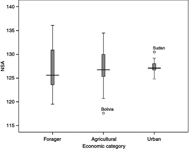
Distributions of the NSA in the three economic categories.
The second trend was a small increase in mean NSA across the three economic categories: foragers (n = 26) 126.5°, agriculturalists (n = 46) 127.3°, and urban (n = 12) 127.8°. These differences in NSA between the economic categories are less pronounced than those reported by Anderson & Trinkaus (1998): foragers (n = 5) 125.1°, agriculturalists (n = 16) 127.5°, and urban (n = 9) 131.5° – although those findings were based on smaller samples and included data from other published sources where techniques may have varied (with at least some data deriving from radiographic measurements). Also, their five forager samples included one pre-Holocene group from the last ice age (NSA 124.5°), whereas their urban samples were defined more strictly than in the present study, being limited to fully mechanized, industrial-era groups. However, if the urban samples here are similarly defined, the resulting seven samples – China (Beijing), France (Paris), Russia (Moscow), the two very recent (cadaveric) Thai samples from Bangkok and Chiang Mai, Ukraine (Kiev), and Venezuela (Caracus) – yield an increase in NSA of only 0.1°, from 127.8 to 127.9°. Nonetheless, a modest trend for increasing NSA associated with the economic transitions from foraging to agricultural and then urban lifestyles is evident. This trend may reflect reduced mechanical loading across the hip joint due to differing habitual activity levels during early development (Anderson & Trinkaus, 1998), or possibly climatic and other thermal factors which may relate to body shape and hence to forces on the hip joint that would affect the NSA. As mentioned above, agricultural and especially urban lifestyles are associated with increased cultural buffering from climate. This could explain the observed narrowing of the NSA range in these categories, in addition to a slight increase in NSA across the economic categories. The routine use of thermally effective clothing will result in a warmer microclimate for the human body, reducing adaptive selection pressures for a stocky, cold-adapted body build and thus leading to an increase in the NSA on thermal grounds.
Within the forager category, the NSA showed a clear climatic trend (Fig. 2), with a strong correlation (r = +0.787) for winter temperature. Climatic correlations were maintained among the agricultural groups, seen for instance with winter temperature (r = +0.437, shown in Supporting Information Fig. S4), but sensitivity to climate was diminished compared with the forager groups. Similarly, correlations between NSA and climate were maintained in the urban groups, seen again for instance with winter temperature (r = +0.787) but, compared with agricultural and especially forager groups, the range of variation was further reduced (shown in Supporting Information Fig. S5).
Fig. 2.
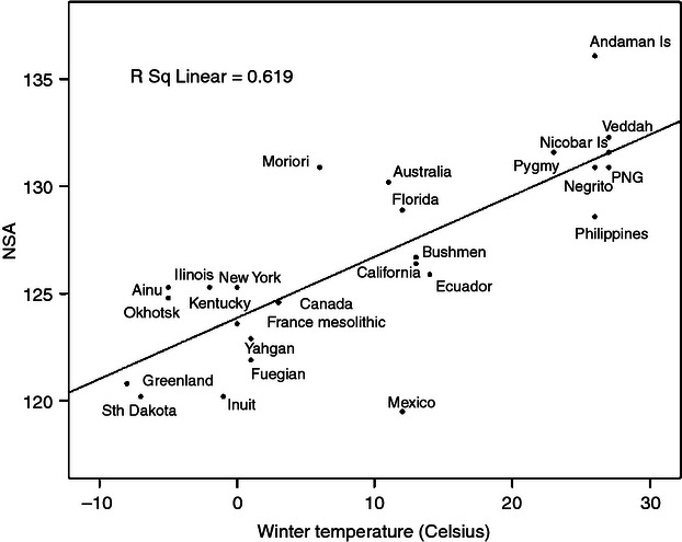
NSA and winter temperature for the forager groups.
Mobility and NSA
The distributions of NSA among the mobile (n = 29) and sedentary (n = 57) groups are shown in Fig. 3. Compared with mobile groups, the NSA was somewhat higher but more restricted in range among the sedentary groups, and this restricted range occurred despite a larger sample size and exposure to a similar range of environmental temperatures (shown in Supporting Information Fig. S6); improved insulation from climatic fluctuations among sedentary groups could account for this trend. The two outliers (Aleutians and the Bolivian sample) were similarly explicable on thermal grounds: low NSA values reflecting, on the Aleutian Islands, cold stress in a high latitude environment and, in the case of Bolivia, cold stress in a high altitude environment. Within mobile groups, the NSA showed a climatic trend (shown in Supporting Information Fig. S7), with a Pearson correlation of r = +0.518 between NSA and winter temperature. Similarly, positive correlations between NSA and environmental temperatures were maintained among the sedentary groups (shown in Supporting Information Fig. S8), with a correlation of r = +0.548 between NSA and winter temperature.
Fig. 3.
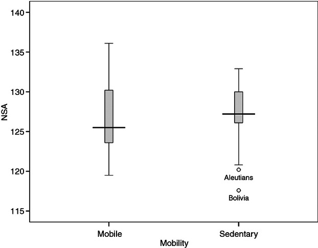
Distributions of the NSA in the mobile and sedentary groups.
Clothing, economy, and mobility
The distributions of clothing codes in the economic and mobility categories were examined for trends in the overall levels of clothing and for differences in thermally relevant aspects – the form of clothing (simple or complex) and the clothing material (e.g. animal hides or woven textile fibres). The distributions of clothing codes in the three economic categories are shown in Fig. 4. An absence or non-routine use of clothing was limited almost entirely to forager groups; the one exception occurred with a predominantly agricultural sample (the Dominican Republic, where the main indigenous group, the Taíno, were habitually unclad but wove cotton for items such as mats and ropes). Forager groups were distinguished from agricultural and urban groups also by an absence of complex (fitted) clothing made of woven textiles, although quite a number of forager groups used simple (draped, single-layer) garments made from woven fibres. Overall, forager groups were characterized by a minimal or reduced level of thermally effective clothing and so, in this important regard, foragers utilized substantially less cultural buffering from the climate than agricultural or urban groups.
Fig. 4.
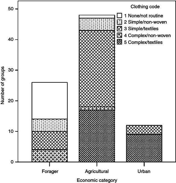
Distributions of clothing codes in the economic categories.
Another trend was the dominance of woven fabrics in the agricultural and urban samples, with the latter groups using exclusively textile garments. The thermal significance of this trend relates to the flexibility and ‘breathability’ of woven garments, facilitating the comfortable and more continuous use of at least some clothing in all climatic conditions (including warm and humid climates) and resulting in a more uniformly warm microenvironment around the human body. However, agricultural and urban groups differed according to the relative proportions of simple (draped) and complex (fitted) clothing: the majority (60%) of agricultural groups used predominantly simple clothing, whereas the majority (75%) of urban groups used more thermally effective complex clothes.
The clear overall trend for clothing in the economic categories was for greater use of clothing in agricultural and urban groups than in the forager groups, with more thermally effective clothing in agricultural and, especially, in urban groups. These differing distributions of clothing codes in the economic categories were statistically significant (results of chi-square tests are given in Supporting Information Table S6). In terms of clothing as ‘cultural buffering’ from the environment, the transitions from forager to agricultural and from agricultural to urban economies were each associated with an increasing degree of insulation from the thermal stresses of climatic variation.
Comparing mobile and sedentary groups, the differences in clothing were less striking than between the three economic categories but were nonetheless statistically significant (shown in Supporting Information Fig. S9 and Table S7). The absence or non-routine use of clothing was more commonplace among mobile groups, and the routine use of clothing of any description was more common among sedentary groups (91%) than mobile groups (72%). Simple clothing was equally common in mobile and sedentary groups (48 and 49%, respectively), whereas complex clothing was more common in sedentary (42%) than in mobile groups (24%). Overall, there was a marked trend for more use of clothing in general, and more use of complex clothing, among the sedentary groups. These clothing trends for mobility were not as strong as for the economic categories, consistent with less pronounced trends in NSA variation between the mobility categories compared with the economic categories.
Clothing and NSA
The distributions of the group NSA means among the five clothing codes are shown in Fig. 5. Two trends were evident: the first was a markedly reduced range in NSA associated with complex clothing, and the second was a slight reduction in average NSA with greater use of clothing. The first trend was more prominent: a narrowing of the NSA range with complex clothing, reflecting more effective buffering from climate. The second trend – a slightly lower NSA with greater use of clothing – probably reflects an underlying climate effect (with cooler climates being associated with more use of clothing and also a lower NSA). Another trend concerned the use of woven textiles for clothing: for both simple and complex clothing, there was a narrowing of the NSA range associated with the use of woven materials. Comparing the environmental temperature ranges associated with the clothing codes (Fig. 6), it becomes clear that this narrowing of the NSA range with complex clothing cannot be attributed to a narrower climatic range: on the contrary, complex clothing was used not only in cooler climates but also across a greater range of mean winter temperatures. The small number of groups using non-woven complex clothing (such as the Ainu and Sami) constituted a specialized case: forager groups using hides and furs for portable warmth in cold environments. Another trend with complex clothing was an association with lower winter temperatures, reflected in the slightly lower NSA among these groups.
Fig. 5.
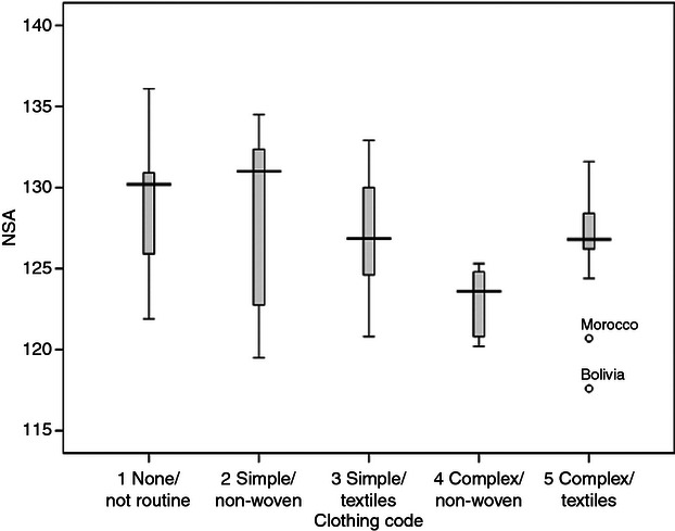
NSA variation among the clothing codes.
Fig. 6.
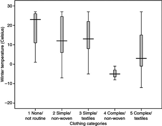
Winter temperature variation for the clothing codes.
Multiple regression analysis
Results of the hierarchical regression analysis are shown in Table 2. This analysis first examines (in Block 1) the independent contribution of the climate variable that correlated most strongly with NSA (winter temperature), while controlling for the effects of the other independent variables (clothing, economy and mobility). In Block 2, these other variables are added, to assess how much remaining NSA variance can be explained. In the Spss output, the power of each block to predict scores on the dependent variable is indicated by the R2 value. The output also provides analysis of variance (anova) to assess the statistical significance of the results and standardized β coefficients to compare the contributions from each independent variable. The R2 values indicated that only a small proportion of total variance in NSA was explained by this analysis – 5.06% with winter temperature as the sole independent variable (Block 1) and 5.34% with the addition of the remaining independent variables (clothing, economy and mobility) in Block 2. However, to achieve adequate sample size, the regression analysis differs from the correlation analyses in needing to use data from individual femora rather than group means, as discussed above. There is much greater variability in the NSA scores when using individual femora rather than group means, and the resulting higher variability in the NSA compared to the independent variables has reduced the power of the regression analysis to detect trends in the NSA at the population level. This is reflected in the very modest R2 values; in contrast, the correlation analyses – using group means – yielded R2 values around 20%. The R2 change of 0.28% shows that addition of the other three independent variables adds only marginally to the variance explained. Nonetheless, this small R2 change of 0.28% reaches statistical significance (P < 0.001), indicating these variables – clothing, economy, and mobility – together increased the predictive power of the model significantly after controlling for the effect of the winter temperature variable. The β coefficients represent the unique contribution of each variable after the overlapping effects of other variables are removed, and hence they under-represent the overall contribution of each independent variable – especially where there exists considerable collinearity between the independent variables, as occurs in this analysis. Two of the β coefficients reached statistical significance: winter temperature (P < 0.001) and clothing (P < 0.05).
Table 2.
Summary table of multiple regression results
| Block 1 | Block 2 | β | Significance | |
|---|---|---|---|---|
| Dependent variable | NSA | NSA | ||
| Independent variable(s) | Winter temperature | Winter temperature | 0.227 | < 0.001** |
| Clothing | 0.037 | 0.024* | ||
| Economy | 0.023 | 0.130 | ||
| Mobility | −0.004 | 0.790 | ||
| R | 0.225 | 0.231 | ||
| R2 | 0.0506 | 0.0534 | ||
| R2 change | 0.0028** |
Significance levels:
P < 0.05,
P < 0.001.
Sex
While 33 groups had sex assigned, only the Thai (Bangkok and Chiang Mai) samples – recent skeletal collections from known persons – provided definite sex determination. For the remainder, sex had been assigned to the femoral specimens based on anatomical assessments involving established osteological criteria for determining sex from associated skeletal elements (e.g. the cranium and pelvis) rather than from the femora themselves, for which femoral head diameter offers the sole accepted anatomical correlate of sex. The present analyses utilized the sex assigned to the specimens by other researchers at the various institutions (e.g. Farewell & Molleson, 1993). Results for the combined total sample (n = 3348) from groups with known or assigned sex are shown in Table 3. There was clearly no sex difference in the NSA using this very large sample, with males and females having the same mean NSA (125.2°) and an identical median NSA (125°).
Table 3.
Descriptive statistics for NSA and sex using the total sample
| Male | Female | ||
|---|---|---|---|
| n | 1882 | 1466 | |
| Total n | 3348 | ||
| % of total | 56.2% | 43.8% | 100 |
| Mean NSA | 125.21 | 125.17 | |
| Difference | 0.04 | ||
| Median | 125 | 125 | |
| Minimum | 108 | 105 | |
| Maximum | 144 | 142 | |
| Range | 36 | 37 | |
| Standard deviation | 5.554 | 5.687 | |
| Standard error of mean | 0.128 | 0.149 | |
| t-test (3346 df) | |||
| Significance (two-tailed) | 0.851 | ||
| % of NSA variance explained by sex | 0.001% | ||
Another strategy for investigating sex differences involved examining the groups separately, comparing the number of groups with differing means for females and males and assessing the magnitude of any sex difference in NSA at the group level. Of the 33 groups with assigned sex, 13 were excluded from group comparisons due to inadequate sampling (< 5 femora for either sex). Comparing the remaining 20 groups (shown in Supporting Information Table S8), approximately half showed females having a slightly higher NSA than males, and half showed an opposite trend (11/20 having the mean female NSA higher than the male mean, and 9/20 having the reverse trend). The average sex difference among these 20 groups was small (0.8°) and, given the mixed group trends, this alternative method for assessing sex difference using group samples likewise indicated no sex difference in the NSA. Three of the group samples were of particular value: the two Thai samples due to definite sex determination and the English (Poundbury) sample by virtue of its sheer size (n = 1271). The differences between male and female NSA in the Bangkok, Chang Mai and Poundbury samples were minor: 0.1, 0.4 and 0.1°, respectively.
Age
Three samples provided data on age: the two Thai samples (where age at death was known) and the Poundbury sample, where age at death was estimated using a combination of skeletal indices (Farewell & Molleson, 1993) The mean ages and the correlations with NSA for these samples, considered separately and combined, are given in Supporting Information Table S9. All of the correlations were slightly negative, suggesting perhaps a slight trend towards a marginal lowering of the NSA during adult life, but none of the correlations approached statistical significance despite adequate sample sizes. Moreover, there was considerable fluctuation within each of the samples and when all three samples with age data were combined, evidence for any overall change in NSA with advancing age was lacking (Fig. 7).
Fig. 7.
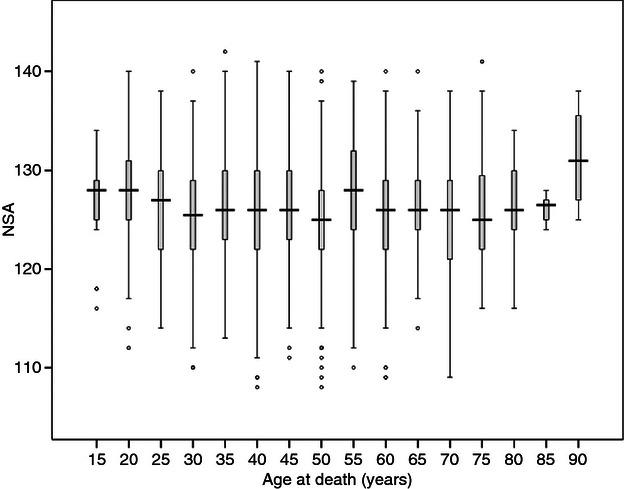
Age distributions of NSA for the combined samples.
Bilateral (left–right) asymmetry
The possibility of a lateral difference in NSA was explored first by examining the complete (n = 8271) femoral database; descriptive statistics for this total sample are shown in Table 4. These findings revealed a modest (1.3°) but statistically significant side difference for the NSA in the total sample. This result was unexpected and warranted closer scrutiny to assess its morphological validity and, as with sex and age, one method for assessing this side difference was to examine the group samples for evidence of a consistent trend. To reduce unreliability associated with small sample sizes, only groups with n ≥ 5 for both left and right femora were included; the results for these 62 groups are shown in Supporting Information Table S10. In contrast to the even distribution of group findings for sex, the group NSA findings for lateral asymmetry showed a consistent difference (left > right) for the majority of groups (52/62). The average difference was 1.7° and, whereas the average side difference in groups where the right NSA exceeded the left was small (0.4°), the average side difference in groups where the left exceeded the right was 2°.
Table 4.
Descriptive statistics for left and right NSA using the total sample
| Left | Right | ||
|---|---|---|---|
| n | 4141 | 4130 | |
| Total n | 8271 | ||
| % of total | 50.07% | 49.93% | 100 |
| Mean NSA | 127.02 | 125.71 | |
| Difference | 1.31 | ||
| Median | 127 | 126 | |
| Minimum | 108 | 105 | |
| Maximum | 148 | 145 | |
| Range | 40 | 40 | |
| Standard deviation | 5.356 | 5.693 | |
| Standard error of mean | 0.083 | 0.089 | |
| t-test (8236 df) | |||
| Significance (two-tailed) | < 0.001* | ||
| % of NSA variance explained by asymmetry | 1.396% | ||
P < 0.001.
This bilateral variation in NSA was then explored using two further strategies: the first utilized a well provenanced regional sample (the mainland USA) and the second examined for asymmetry at the individual level, using matched femora. The regional findings yielded quite compelling evidence for bilateral asymmetry (Table 5), with left > right in the majority (7/8) of groups and an average side difference of 3° among the mainland USA groups; the large Inuit sample from the Aleutian Islands showed a similar side difference (2.9°). Asymmetry was evaluated also at the individual level (see Auerbach & Ruff, 2006) by comparing the distribution of differences between the left and right NSA in matched femoral pairs. The total database included 4592 NSA measures from matched femora, and the left–right difference was calculated for each of the individual pairs. These results showed a modest mean difference of 1.03° (left > right) and a median difference of 1° (n = 2296 paired femora). The distributions were skewed to the left: 55% (1273 pairs) showed left > right, 34% (778 pairs) showed right > left, and 11% (245 pairs) showed left = right. Paired t-test results indicated that the side difference in NSA for matched femoral pairs was significant: t = 13.842, 2295 df, significance (two-tailed test) P < 0.0005. This finding of a left bias at the level of individual femoral pairs, when considered in conjunction with the reasonably consistent side difference found among the regional/group samples and across the total femoral sample, provides collective evidence for minor lateral asymmetry in the NSA (approximately 1–3°, left > right) at the population level.
Table 5.
Left–right side differences in NSA among the USA samples
| Left | Right | |||||
|---|---|---|---|---|---|---|
| State/Sample | n | NSA | n | NSA | n | Difference (right–left) |
| USA (excluding Aleutian Islands) | ||||||
| California/Chumash | 78 | 125.9 | 41 | 126.8 | 37 | +0.91 |
| Florida/(Various) | 306 | 131.0 | 154 | 126.7 | 152 | −4.25 |
| Illinois/Woodland | 100 | 126.7 | 52 | 123.8 | 48 | −2.90 |
| Kentucky/Archaic | 129 | 125.6 | 65 | 121.7 | 64 | −3.89 |
| Louisiana/Mississippian | 118 | 128.8 | 52 | 124.8 | 66 | −4.01 |
| New Mexico/Hawikuh | 142 | 125.2 | 70 | 121.7 | 72 | −3.52 |
| New York/Manhattan Island | 13 | 126.9 | 7 | 123.5 | 6 | −3.36 |
| South Dakota/Arikara | 101 | 121.7 | 48 | 118.9 | 53 | −2.84 |
| Summary | ||||||
| Right > left | 1/8 | |||||
| Average difference (sample means) | −2.98 | |||||
Other femoral measures
Where possible, data on three additional femoral variables were collected: femoral head diameter (FHD), bicondylar breadth (BCB), and maximum femoral length (MFL). FHD is recognized widely as a skeletal correlate of body mass and sex (e.g. Auerbach & Ruff, 2004; Stock & Pfeiffer, 2004) and was analyzed here in relation to sex, climate, and the NSA; BCB also has weight-bearing aspects and, similarly, is a skeletal correlate of body mass. MFL, on the other hand, serves as an osteological correlate of stature and, to a lesser extent, sex (e.g. Brothwell, 1981; Kondo et al. 2000; Holliday, 2002), but not body mass.
Results for these other femoral variables are provided in Supporting Information Data S1. Briefly, FHD showed a statistically significant sex difference, and its value as an index of body mass was reflected in significant climatic trends, consistent with Bergmann's rule. Additionally, FHD correlated significantly with NSA. The findings for BCB – like FHD, a proxy for body mass – paralleled those for FHD. MFL showed a marked sex difference, reflecting its utility as an estimate for stature. However, MFL did not correlate with climate (or with NSA). This is again consistent with principles based on Bergmann's rule: changes in stature alone do not affect the surface area/mass ratio, and previous studies have shown that stature does not correlate with climate (using latitude as a climatic proxy) among modern humans (Ruff, 1994). There was, however, a small but statistically significant side difference with MFL: the mean left MFL was 1.66 mm greater than mean right MFL. This finding of bilateral asymmetry in MFL corroborates the finding in this study of bilateral asymmetry in the NSA, given that a lower right NSA should lead to a slightly shorter right femur. There is little suggestion in the literature that bilateral asymmetry exists for MFL: limb length asymmetry is generally more marked in upper than lower limbs, although a small bilateral difference in MFL (with the left femur averaging approximately 1 mm longer than the right) was reported in a sample of 780 femoral pairs (Auerbach & Ruff, 2006).
Discussion
These analyses revealed significant climatic trends for the NSA among modern humans at the global level with, for instance, a generally lower average NSA among groups occupying cooler environments. Of four climatic indices (latitude and mean annual, summer, and winter temperatures), the strongest correlations occurred with mean winter temperature, reflecting the role of cold stress in human morphological adaptation to climatic variation. The highest average NSA occurred in the Pacific region, with Asia and Africa also having continental NSA values above the global mean, which was found to be approximately 127° (126.4° as measured across the entire sample of 8271 femora and 127.4° when measured over the 100 group samples). This average NSA among modern humans of 127° is markedly lower than the average angle of 135° quoted, for instance, in Gray's Anatomy (Standring, 2008). The difference may be attributable to the extensive use of radiographic measurements in previous studies, which would significantly exaggerate the NSA. Lower mean NSA values have been reported previously using direct measurement: for example, 126.3° (n = 120) and 126.7° (n = 50) for two overlapping Pecos Pueblo samples from North America (Ruff, 1981; Anderson & Trinkaus, 1998).
In relation to continental variation in the NSA, the European means (126.3° using individual femora, 125.3° using groups, average mean 125.8°) fell a little below the global average, with the Americas having the lowest NSA means: average 124.5° for North America and 124.8° for South America. The latter yielded the lowest group sample mean (117.6°), which derived from the high-altitude Lake Titicaca area in Bolivia. The relatively low American NSA (average 124.6° for both continents) is likely a consequence of selection pressure for cold adaptation (and hence for a more stocky body shape) among the ancestors of Native Americans, who migrated from northeastern Eurasia towards the end of the last ice age (e.g. Turner, 2002; Auerbach, 2012).
Similarly, other continental and regional differences in the NSA may reflect the differing thermal environments (and the differing environmental histories) of the local populations. The Pacific samples (average mean 129.8°) comprised approximately half Melanesian and half Polynesian groups (with Micronesia being represented only by two very small samples, from Kiribati and Guam). Melanesians have a long history (and prehistory extending at least into the late Pleistocene) within the tropics, while Polynesians have their mid-Holocene origins in Melanesia and southeastern Asia (e.g. Bellwood, 1979; White & Allen, 1980). The African mean NSA (average 127.9°) was above the global average, with tropical and subtropical parts of the continent being well represented in the group samples. The Asian mean (average 128.7°) was also relatively high, which may be due to a majority (14/24) of the Asian samples deriving from the tropics, with only a quarter (6/24) deriving from cooler temperate environmental zones – China (a single sample from northern China), Japan, Nepal, the Russian Far East and the Ainu and Okhotsk groups. The routine use of thermally effective clothing among most of these latter six groups might also ameliorate any climatic influence: all have relatively high NSA values (the Russian Far East having the highest, 130°). Relatively lower NSA group means were found in Europe, as was a narrower NSA range compared with other continents, with the latter reflecting a more restricted geographical range in terms of latitude (and hence a more restricted range of temperatures).
Among the ‘other’ groups considered separately from national affiliations, a number are noteworthy for their comparatively extreme mean NSA: the Andaman Islanders (136.1°, n = 81), the Inuit (120.2°, n = 324), and the Fuegians (122.4°, n = 34). A low NSA for the Inuit sample suggests considerable cold exposure (and wind chill effect) in their maritime environment on the Aleutian Islands (Alaska), despite the use of sophisticated clothing (e.g. Issenman, 1997). Conversely, clothing was absent among the Andaman Islanders prior to British settlement (e.g. Mouat, 1863) and their high NSA reflects long-term morphological adaptation to a quite uniformly warm thermal environment (mean annual and summer temperatures of 27 °C, mean winter temperature 26 °C). At the other climatic extreme, on the southernmost tip of South America, the low mean NSA among the Fuegians reflects both their cold environment and their limited use of clothing: early European observers were astonished by how the local inhabitants managed to survive in the cold conditions with only minimal protection in the form of simple capes and cloaks, often wearing nothing at all (e.g. Darwin, 1839).
With regard to lifestyle patterns, there was a modest trend towards increasing mean NSA with the transitions from forager to agricultural and urban lifestyles and, to a lesser extent, from a mobile to a more sedentary existence. The most noticeable trend, though, was a progressive narrowing in the NSA range associated with these transitions, which could be due to increased cultural buffering from the environment. It may be argued, on the other hand, that this observed difference in NSA variability is attributable to an effect of sample size. In particular, the narrow range in the urban category could reflect a reduced urban sample size (n = 12) compared with the forager (n = 26) and agricultural (n = 46) samples. However, the NSA range is similarly reduced among the agricultural groups compared with foragers, despite a larger sample size for agriculturalists (n = 46, vs. n = 26). Also, the range of NSA variation is likewise reduced in the sedentary groups compared with the mobile groups, and this occurs despite the sample size for agriculturalists being larger (n = 57) than for the mobile groups (n = 29). There is, in other words, a consistent trend for reduced NSA variation in agricultural, urban, and sedentary populations, and this trend is seen to occur regardless of relative sample size. These findings cast doubt on whether the narrow range of NSA variation found among urban groups can be considered to simply reflect a smaller sample size. Instead, cultural buffering from climate – including the insulating effect of clothing – is implicated in these observed relationships between lifestyle and NSA variation. Specifically, the clothing analyses demonstrate that greater use of more thermally effective clothing is associated with agricultural, urban, and sedentary lifestyles. Clothing thus emerges as a confounding variable in the NSA trends for economic activity and mobility. The thermal effect of clothing can account for the increase in NSA observed among more sedentary, mechanized societies and also – a finding that provides the strongest evidence – the progressive narrowing of the NSA range, which is most likely due to increased thermal insulation. An underlying climate effect on NSA is nonetheless discernible despite the buffering effect of clothing: climatic trends are preserved within each of the economic and mobility categories, with a cooler climates associated with a reduction in mean NSA.
The multiple regression analysis highlighted climate (mean winter temperature) as the dominant independent variable affecting NSA (P < 0.001), with the clothing and lifestyle variables contributing a marginal improvement in predictive power. Of the latter, only clothing emerged as statistically significant (at the P < 0.05 level). The effect of clothing was small yet statistically significant in its own right, whereas neither economy nor mobility made a statistically significant unique contribution. The multiple regression results showed that collinearity between clothing, economy, and mobility was substantial, compromising assessment of the relative contributions made by these variables to variation in the NSA. However, any effects of economy and mobility on NSA variation may be mediated by their systematic association with clothing which, as discussed above, may act as a confounding factor in the observed NSA trends associated with lifestyle among modern human groups.
The analyses demonstrated no sex difference in the NSA (cf. Standring, 2008) and no evidence was found for any consistent change associated with advancing age. The one unexpected anatomical finding was a small but consistent (and statistically significant) difference between the left and right NSA, with the right femur having a slightly lower NSA (by 1.3°) than the left femur, averaged across the whole database. The likely reliability of this result was suggested by finding a comparable left–right difference (averaging ∼ 2°) among the great majority (52/62) of groups with adequate sample sizes (n ≥ 5 for both left and right femora). A regional sampling of mainland USA groups gave a similar result: the mean left NSA exceeded the mean right NSA in the majority (7/8) of the groups, with an average bilateral NSA difference of ∼ 3°. Results from matched femoral pairs (n = 2297) also indicated a left bias (∼ 1°). Asymmetry in femoral NSA is hitherto unreported, although asymmetry has been reported in femoral anteversion, which was found to be greater on the right side (21°) than on the left (17°) in a single sample (n = 228) of African femora (Eckhoff et al. 1994).
The question arises as to possible reasons for asymmetry in the NSA. One candidate is leg dominance: a side difference in limb preference is well documented not only in modern humans but in other animal species, with the right leg dominant in most modern-day humans studied (e.g. Bell & Gabbard, 2000; Lenoir et al. 2006). This right-sided leg dominance may place greater biomechanical stresses on the right femoral neck during childhood development (when the NSA reduces markedly due to biomechanical loading). Right leg dominance could contribute a small additional effect independently of factors associated with body shape (and the associated climatic trends), leading to a slightly lower average right NSA at the population level. However, right leg dominance does not necessarily place greater mechanical loading on the right femoral neck: leg dominance refers more to motor coordination, with the non-preferred (left) leg possibly subjected to greater mechanical loading as the stabilizing or weight-bearing limb (Auerbach & Ruff, 2006). In that case, it becomes more difficult to understand how right leg dominance would tend to result in a lower right NSA. If a relationship does exist between leg dominance and lateral variation in the NSA, the mechanisms involved may be more complex than presently understood. Insofar as leg dominance might be implicated, it could also be accentuated by any activity effect on the NSA, with higher habitual activity levels placing greater loads on the right – in most cases, the dominant – femur. Habitual activity probably exerts a relatively minor influence on NSA compared with the effects of body shape and climate (at least as shown by the findings reported here) but biomechanical forces across the hip joint are nonetheless implicated as underlying the relationship between body shape and NSA (Weaver, 2003; see also Ruff & Higgins, 2013).
Lastly, results for the additional femoral variables measured in this study (FHD, BCB, and MFL) collectively provide independent support for the NSA findings. FHD and BCB correlated with climate (and with NSA), whereas MFL showed no correlations with climate. These findings are interpreted as reflecting anatomical relationships with the climatic indices based on Bergmann's rule.
Limitations
These analyses have utilized relatively simple climatic indices: latitude, mean annual temperature, and mean monthly summer and winter temperature. While this represents an improvement over other studies that have used latitude as the sole climatic index (e.g. Anderson & Trinkaus, 1998), additional meteorological variables – such as average maximum and minimum temperatures and, ideally, more physiologically meaningful indices of thermal stress such as wind chill and apparent temperature (e.g. Steadman, 1984; Quayle & Steadman, 1998) – would provide superior measures of local thermal conditions and hence better assessments of environmental selection pressures. However, adequate meteorological records to facilitate such analyses were not available for the vast majority of geographical locations. Perhaps surprisingly, given that latitude is a crude approximation for average thermal conditions, the NSA correlated significantly with latitude at the global level (although stronger correlations were seen with mean annual and mean winter monthly temperatures).
This study benefited not only from its large sample size and extensive geographical coverage but also from its consistent and relatively reliable method for estimating the NSA – namely, all measurements were determined visually by a single observer using a hand-held goniometer on the femora themselves. Although this method has the advantage of simplicity, and published inter- and intra-observer error margins are acceptably minimal (typically 1–2°; Anderson & Trinkaus, 1998), there is nonetheless a certain degree of subjectivity involved. A more accurate approach is to scan the surface of the femur digitally and then apply various statistical regression models to approximate the shape and orientation of the femoral neck in three dimensions. Using this digitizing technology, Bonneau et al. (2012) found that the femoral neck is best modelled using successive cross-sectional ellipses, with the femoral neck axis being computed from the centres of the ellipses. Their sample of 91 modern European (French and Swiss) femora showed a significant sex and age effect on anteversion (greater in females, and reducing with age) but, notably, no effects of sex, age nor laterality for the NSA. They advocated using this digital methodology to explore the three-dimensional femoral neck orientation across a wide range of human populations, examining specifically for possible variation relating to differing habitual activity patterns, geographical origins, and environments. This would certainly be a worthwhile endeavour given the results obtained here using a simpler methodology, although it would entail greater resources to obtain the quality of sampling required to replicate the present study.
Conclusions
Although these findings have demonstrated high variability of the femoral NSA at the individual and group levels among modern humans, the unprecedented size and global scope of this study has demonstrated that NSA variation at the population level correlates with climate, consistent with well documented climatic trends in other indices of human body shape based on principles derived from Bergmann's rule. The mean NSA for modern humans is 127°, with variation in regional median values reflecting climatic conditions: the Pacific median is 130°, Asia 129°, Africa 127°, Europe 126°, and the Americas 125°. Variation relating to differing routine activity patterns associated with major lifestyle (economy and mobility) categories is less pronounced, with a possible confounding effect of the habitual use of clothing due to its systematic association with the lifestyle variables. An independent thermal effect of clothing as cultural buffering from climate is evident in the reduced environmental sensitivity of the NSA associated with more sophisticated forms of clothing. These results show a predominant thermal basis for variation in the NSA at the population level due to the effects of climate and clothing. Extensive sampling has also allowed specific anatomical questions to be answered, notably with the unexpected finding of a small side difference in the NSA and the absence of a sex difference.
Acknowledgments
The authors thank David Bulbeck, Colin Groves, David Leask, Bill Lyndon, Marc Oxenham, Colin Pardoe, and Peter White for their assistance during the course of this research, and Erik Trinkaus for his advice on measuring femoral neck-shaft angles. Robert Attenborough, Nicholas Babidge, Kevin Clarke, Patrick Guinness, Matthew Large, and Maryanne O'Donnell provided support for preparation of the paper. We also express our gratitude to the curators, managers, and other staff who facilitated access to the collections (listed alphabetically by institution): Gisselle Garcia (American Museum of Natural History, New York), Donna Ruhl (Florida Museum of Natural History), Henry de Lumley, Amélie Vialet, and Stéphanie Renault (Institut de Paléontologie Humaine, Paris), Mercedes Okumura (Leverhulme Centre for Human Evolutionary Studies, Cambridge), Philippe Mennecier and others – notably Aurélie, Véronique, and Liliana – at the Museé de l'Homme (Paris), Reiko Kono (National Museum of Nature and Science, Tokyo), Robert Kruszynski (Natural History Museum, London), Olivia Herschensohn (Peabody Museum, Harvard University), Hirofumi Matsumura (Sapporo Medical University), David R. Hunt (Smithsonian Institution, Washington, DC), Keryn Walshe and Rebekah Candy (South Australian Museum), and Eric Cook (Indigenous representative for Roonka). This work was supported by a University House Postgraduate Research Scholarship, a Fieldwork Grant from the Faculty of Arts and a Postdoctoral Research Fellowship from the College of Arts and Social Sciences, Australian National University.
Author contributions
I.G.: Responsible for study design, data acquisition, analysis and interpretation, and drafting the paper. S.C.: Substantial contribution to data acquisition, namely during the pilot study in Thailand, where important practical aspects of the study were finalized, including assessing the suitability of skeletal material for inclusion, and determining appropriate measurement techniques. P.M.: Substantial contribution to study methodology and data acquisition (notably, advising on measurement issues and techniques), and critical revision of the paper.
Supporting Information
Additional Supporting Information may be found in the online version of this article:
Data S1. Other femoral variables.
Fig. S1. Normal probability plot.
Fig. S2. Residuals scatter plot.
Fig. S3. Distributions of winter temperatures for the three economic categories.
Fig. S4. NSA and winter temperature for the agricultural groups.
Fig. S5. NSA and winter temperature for the urban groups.
Fig. S6. Winter temperature ranges for the mobile and sedentary groups.
Fig. S7. NSA and winter temperature for the mobile groups.
Fig. S8. NSA and winter temperature for the sedentary groups.
Fig. S9. Distributions of clothing codes in the mobility categories.
Fig. S10. Distributions of FHD for males and females.
Fig. S11. Distributions of male and female BCB.
Fig. S12. Distributions of male and female MFL.
Fig. S13. Distributions of male MFL and winter temperature.
Table S1. Number of femora measured (n) at each of the participating institutions (listed alphabetically), and number of countries, territories, and other groups sampled.
Table S2. List of each sample group with the assigned weather station, latitude (°N/S), and associated climatic data: mean annual (A) temperature, and mean monthly summer (S) and winter (W) temperatures (°C).
Table S3. Group codes for economy and mobility, and corresponding Murdock codes.
Table S4. Descriptions and examples of the five clothing codes.
Table S5. Clothing codes for the 86 lifestyle sample groups.
Table S6. Results of chi-square tests for clothing and economy.
Table S7. Results of chi-square tests for clothing and mobility.
Table S8. Sex differences in mean NSA among samples with n ≥ 5 for both sexes.
Table S9. Mean age and correlations between NSA and age for the Bangkok, Chiang Mai, total Thai, Poundbury, and combined samples.
Table S10. Side differences for groups with n ≥ 5 for both left and right NSA.
Table S11. Correlations and results of significance tests for FHD and the climatic indices.
Table S12. Correlations and results of significance tests for FHD and NSA.
Table S13. Correlations and results of significance tests for BCB and the climatic indices.
Table S14. Correlations and results of significance tests for BCB and NSA.
Table S15. Descriptive statistics and results of t-test for left and right MFL.
Table S16. Bilateral asymmetry in FHD and BCB.
References
- Allen JA. The influence of physical conditions in the genesis of species. Rad Rev. 1877;1:108–140. [Google Scholar]
- Anderson JY, Trinkaus E. Patterns of sexual, bilateral and interpopulational variation in human femoral neck-shaft angles. J Anat. 1998;192:279–285. doi: 10.1046/j.1469-7580.1998.19220279.x. [DOI] [PMC free article] [PubMed] [Google Scholar]
- Ashton KJ, Tracy MC, de Queiroz A. Is Bergmann's rule valid for mammals? Am Nat. 2000;156:390–415. doi: 10.1086/303400. [DOI] [PubMed] [Google Scholar]
- Auerbach BM. Skeletal variation among early Holocene North American humans: implications for origins and diversity in the Americas. Am J Phys Anthropol. 2012;149:525–536. doi: 10.1002/ajpa.22154. [DOI] [PubMed] [Google Scholar]
- Auerbach BM, Ruff CB. Human body mass estimation: a comparison of ‘morphometric’ and ‘mechanical’ methods. Am J Phys Anthropol. 2004;125:331–342. doi: 10.1002/ajpa.20032. [DOI] [PubMed] [Google Scholar]
- Auerbach BM, Ruff CB. Limb bone bilateral asymmetry: variability and commonality among modern humans. J Hum Evol. 2006;50:203–218. doi: 10.1016/j.jhevol.2005.09.004. [DOI] [PubMed] [Google Scholar]
- Bell J, Gabbard C. Foot preference changes through adulthood. Laterality. 2000;5:63–68. doi: 10.1080/713754351. [DOI] [PubMed] [Google Scholar]
- Bellwood PS. Man's Conquest of the Pacific: The Prehistory of Southeast Asia and Oceania. New York: Oxford University Press; 1979. [Google Scholar]
- Bergmann C. Uber die Verhältniesse der Wärmeokonomie der Thiere zu ihrer Grösse. Göttinger Stud. 1847;1:595–708. [Google Scholar]
- Bonneau N, Libourel P-A, Simonis C, et al. A three-dimensional axis for the study of femoral neck orientation. J Anat. 2012;221:465–476. doi: 10.1111/j.1469-7580.2012.01565.x. [DOI] [PMC free article] [PubMed] [Google Scholar]
- Brothwell DR. Digging Up Bones: The Excavation, Treatment and Study of Human Skeletal Remains. 3rd edn. London: British Museum (Natural History); 1981. [Google Scholar]
- Cavalli-Sforza LL. African Pygmies: an evaluation of the state of research. In: Cavalli-Sforza LL, editor. African Pygmies. Orlando, FL: Academic Press; 1986. pp. 361–426. [Google Scholar]
- Cheng XG, Lowett G, Boonen S, et al. Assessment of the strength of proximal femur in vitro: relationship to femoral bone mineral density and femoral geometry. Bone. 1997;20:213–218. doi: 10.1016/s8756-3282(96)00383-3. [DOI] [PubMed] [Google Scholar]
- Crognier E. Climate and anthropometric variations in Europe and the Mediterranean area. Ann Hum Biol. 1981;8:99–107. doi: 10.1080/03014468100004841. [DOI] [PubMed] [Google Scholar]
- Darwin C. Journal and remarks. 1832–1836. In: Fitz-Roy R, editor. Narrative of the Surveying Voyages of His Majesty's Ships Adventure and Beagle, Between the Years 1826 and 1836, Describing their Examination of the Southern Shores of South America, and the Beagle's Circumnavigation of the Globe. III. London: Henry Colburn; 1839. [Google Scholar]
- Davivongs V. The femur of the Australian Aborigine. Am J Phys Anthropol. 1963;21:457–467. doi: 10.1002/ajpa.1330210404. [DOI] [PubMed] [Google Scholar]
- Doherty M, Courtney P, Doherty S, et al. Nonspherical femoral head shape (pistol grip deformity), neck shaft angle, and risk of hip osteoarthritis. Arthritis Rheum. 2008;58:3172–3182. doi: 10.1002/art.23939. [DOI] [PubMed] [Google Scholar]
- Eckhoff DG, Kramer RC, Watkins JJ, et al. Variation in femoral anteversion. Clin Anat. 1994;7:72–75. [Google Scholar]
- Farewell DE, Molleson TL. Excavations at Poundbury 1966–80. Volume II: The Cemeteries. Dorchester: Dorset Natural History and Archaeological Society; 1993. [Google Scholar]
- Gilligan I. Clothing and farming origins: the Indo-Pacific evidence. Bull Indo Pac Pre Hi. 2007;27:10–24. [Google Scholar]
- Gilligan I. Clothing and climate in Aboriginal Australia. Curr Anthropol. 2008;49:487–495. [Google Scholar]
- Gilligan I. The prehistoric development of clothing: archaeological implications of a thermal model. J Archaeol Method Theory. 2010a;17:15–80. [Google Scholar]
- Gilligan I. Femoral neck-shaft angle and climate: preliminary report on a global study. In: Weiss KE, editor. Trends in Physical Anthropology. Hauppauge, NY: Nova Science; 2010b. pp. 123–152. [Google Scholar]
- Gilligan I. Climatic variation in femoral neck-shaft angle among modern humans: continental and regional trends. In: Sarana G, Srivastava RP, editors. Studies in Social and Physical Anthropology: Essays in Memory of DK Sen. Jaipur: Rawat Publications; 2012. pp. 17–79. [Google Scholar]
- Gilligan I, Bulbeck D. Environment and morphology in Australian Aborigines: a re-analysis of the Birdsell database. Am J Phys Anthropol. 2007;134:75–91. doi: 10.1002/ajpa.20640. [DOI] [PubMed] [Google Scholar]
- Gnudi S, Sitta E, Fiumi N. Bone density and geometry in assessing hip fracture risk in post-menopausal women. Br J Radiol. 2007;80:893–897. doi: 10.1259/bjr/37401526. [DOI] [PubMed] [Google Scholar]
- Gould SJ. Allometry and size in ontogeny and phylogeny. Biol Rev. 1966;41:587–640. doi: 10.1111/j.1469-185x.1966.tb01624.x. [DOI] [PubMed] [Google Scholar]
- Hiernaux J, Rudan P, Brambati A. Climate and the weight/height relationship in sub-Saharan Africa. Ann Hum Biol. 1975;2:3–12. doi: 10.1080/03014467500000511. [DOI] [PubMed] [Google Scholar]
- Holliday TW. Body proportions in late Pleistocene Europe and modern human origins. J Hum Evol. 1997;32:423–447. doi: 10.1006/jhev.1996.0111. [DOI] [PubMed] [Google Scholar]
- Holliday TW. Body size and postcranial robusticity of European upper palaeolithic hominins. J Hum Evol. 2002;43:513–528. [PubMed] [Google Scholar]
- Holliday TW, Falsetti AB. Lower limb length of European early modern humans in relation to mobility and climate. J Hum Evol. 1995;29:141–153. [Google Scholar]
- Houghton P. The adaptive significance of Polynesian body form. Ann Hum Biol. 1990;17:19–32. doi: 10.1080/03014469000000752. [DOI] [PubMed] [Google Scholar]
- Houston CS, Zaleski WA. The shape of vertebral bodies and femoral necks in relation to activity. Radiology. 1967;89:59–66. doi: 10.1148/89.1.59. [DOI] [PubMed] [Google Scholar]
- Igbigbi PS. Collo-diaphysial angle of the femur in East African subjects. Clin Anat. 2003;16:416–419. doi: 10.1002/ca.10148. [DOI] [PubMed] [Google Scholar]
- Issenman BK. Sinews of Survival: The Living Legacy of Inuit Clothing. Vancouver: UBC Press; 1997. [Google Scholar]
- Katzmarzyk PT, Leonard WR. Climatic influences on human body size and proportions: ecological adaptations and secular trends. Am J Phys Anthropol. 1998;106:483–503. doi: 10.1002/(SICI)1096-8644(199808)106:4<483::AID-AJPA4>3.0.CO;2-K. [DOI] [PubMed] [Google Scholar]
- Kondo O, Dodo Y, Akazawa T, et al. Estimation of stature from the skeletal reconstruction of an immature Neandertal from Dederiyeh Cave, Syria. J Hum Evol. 2000;38:457–473. doi: 10.1006/jhev.1999.0347. [DOI] [PubMed] [Google Scholar]
- Lenoir M, van Overschelde S, de Rycke M, et al. Intrinsic and extrinsic factors of turning preferences in humans. Neurosci Lett. 2006;393:179–183. doi: 10.1016/j.neulet.2005.09.061. [DOI] [PubMed] [Google Scholar]
- Levinson D. Ethnic Groups Worldwide: A Ready Reference Handbook. Phoenix: Oryx Press; 1998. [Google Scholar]
- Mayr E. Geographical character gradients and climatic adaptation. Evolution. 1956;10:105–108. [Google Scholar]
- Meiri S, Dayan T. On the validity of Bergmann's rule. J Biogeogr. 2003;30:331–351. [Google Scholar]
- Mouat FJ. Adventures and Researches among the Andaman Islanders. London: Hurst and Blackett; 1863. [Google Scholar]
- Murdock GP. Atlas of World Cultures. Pittsburgh: University of Pittsburgh Press; 1981. [Google Scholar]
- Ogata K, Goldsand EM. A simple biplanar method of measuring femoral anteversion and neck-shaft angle. J Bone Joint Surg. 1979;61:846–851. [PubMed] [Google Scholar]
- Olsen M, Davis ET, Gallie PAM, et al. The reliability of radiographic assessment of femoral neck-shaft and implant angulation in hip resurfacing arthroplasty. J Arthroplasty. 2009;24:333–340. doi: 10.1016/j.arth.2008.01.304. [DOI] [PubMed] [Google Scholar]
- Pate FD. Hunter-gatherer social complexity at Roonka Flat, South Australia. In: David B, Barker B, McNiven IJ, editors. The Social Archaeology of Australian Indigenous Societies. Canberra: Aboriginal Studies Press; 2006. pp. 226–241. [Google Scholar]
- Perneger TV. What's wrong with Bonferroni adjustments. Br Med J. 1998;316:1236–1238. doi: 10.1136/bmj.316.7139.1236. [DOI] [PMC free article] [PubMed] [Google Scholar]
- Pulkkinen P, Eckstein F, Lochmüller E-M, et al. Association of geometric factors and failure load level with the distribution of cervical vs. trochanteric hip fractures. J Bone Miner Res. 2006;21:895–901. doi: 10.1359/jbmr.060305. [DOI] [PubMed] [Google Scholar]
- Quayle RG, Steadman RG. The Steadman Wind Chill: an improvement over present scales. Weather Forecast. 1998;13:1187–1193. [Google Scholar]
- Roberts DF. Climate and Human Variability. Chicago: Cummings; 1978. [Google Scholar]
- Robertson GB, Prescott JR. Luminescence dating at the archaeological and human burial site at Roonka, South Australia. Quat Sci Rev. 2006;25:2586–2593. [Google Scholar]
- Ruff CB. University of Pennsylvania; 1981. Structural Changes in the Lower Limb with Aging at Pecos Pueblo. PhD thesis. [Google Scholar]
- Ruff CB. Climate and body shape in hominid evolution. J Hum Evol. 1991;21:81–105. [Google Scholar]
- Ruff CB. Climatic adaptation and hominid evolution: the thermoregulatory imperative. Evol Anthropol. 1993;2:53–60. [Google Scholar]
- Ruff CB. Morphological adaptation to climate in modern and fossil hominids. Yearb Phys Anthropol. 1994;37:65–107. [Google Scholar]
- Ruff CB. Variation in human body size and shape. Annu Rev Anthropol. 2002;31:211–232. [Google Scholar]
- Ruff CB, Higgins R. Femoral neck structure and function in early hominins. Am J Phys Anthropol. 2013;150:512–525. doi: 10.1002/ajpa.22214. [DOI] [PubMed] [Google Scholar]
- Schreider E. Morphological variations and climatic differences. J Hum Evol. 1975;4:529–539. [Google Scholar]
- Standring S, editor. Gray's Anatomy: The Anatomical Basis of Clinical Practice. 40th edn. Edinburgh: Churchill Livingstone; 2008. [Google Scholar]
- Steadman RG. A universal scale of apparent temperature. J Appl Meteorol. 1984;23:1674–1687. [Google Scholar]
- Stock JT, Pfeiffer SK. Long bone robusticity and subsistence behaviour among Later Stone Age foragers of the forest and fynbos biomes of South Africa. J Archaeol Sci. 2004;31:999–1013. [Google Scholar]
- Tabachnick BG, Fidell LS. Using Multivariate Statistics. 6th edn. Boston: Pearson; 2012. [Google Scholar]
- Trinkaus E. Neanderthal limb proportions and cold adaptation. In: Stringer CB, editor. Aspects of Human Evolution. London: Taylor & Francis; 1981. pp. 187–223. [Google Scholar]
- Trinkaus E. Femoral neck-shaft angles of the Qafzeh-Skhul early modern humans, and activity levels among immature Near Eastern Middle Paleolithic hominids. J Hum Evol. 1993;25:393–416. [Google Scholar]
- Trinkaus E. Femoral neck-shaft angles: a reply to Arensburg. J Hum Evol. 1994;27:451–455. [Google Scholar]
- Turner CG. Teeth, needles, dogs, and Siberia: bioarchaeological evidence for the colonization of the New World. In: Jablonski NG, editor. The First Americans: The Pleistocene Colonization of the New World. San Francisco: California Academy of Sciences; 2002. pp. 123–158. [Google Scholar]
- Walensky NA, O'Brien MP. Anatomical factors relative to the racial selectivity of femoral neck fracture. Am J Phys Anthropol. 1968;28:93–96. doi: 10.1002/ajpa.1330280118. [DOI] [PubMed] [Google Scholar]
- Weaver TD. The shape of the Neandertal femur is primarily the consequence of a hyperpolar body form. Proc Natl Acad Sci U S A. 2003;100:6926–6929. doi: 10.1073/pnas.1232340100. [DOI] [PMC free article] [PubMed] [Google Scholar]
- Weinstein KJ. Body proportions in ancient Andeans from high and low altitudes. Am J Phys Anthropol. 2005;128:569–585. doi: 10.1002/ajpa.20137. [DOI] [PubMed] [Google Scholar]
- White JP, Allen J. Melanesian prehistory: some recent advances. Science. 1980;207:728–734. doi: 10.1126/science.207.4432.728. [DOI] [PubMed] [Google Scholar]
Associated Data
This section collects any data citations, data availability statements, or supplementary materials included in this article.