Extracting Global System Dynamics of Corticosteroid Genomic Effects in Rat Liver

Abstract

One of the challenges in constructing biological models involves resolving meaningful data patterns from which the mathematical models will be generated. For models that describe the change of mRNA in response to drug administration, questions exist whether the correct genes have been selected given the myriad transcriptional effects that may occur. Oftentimes, different algorithms will select or cluster different groups of genes from the same data set. A new approach was developed that focuses on identifying the underlying global dynamics of the system instead of selecting individual genes. The procedure was applied to microarray genomic data obtained from rat liver after a large single dose of methylprednisolone in 52 adrenalectomized rats. Twelve clusters of at least 30 genes each were selected, reflecting the major changes over time. This method along with isolating the underlying dynamics of the system also extracts and clusters the genes that make up this global dynamic for further analysis as to the contributions of specific mechanisms affected by the drug.

Corticosteroids are synthetic glucocorticoids used therapeutically for their potent anti-inflammatory, antiproliferative, and immunosuppressive effects (Cronstein et al., 1992; Chikanza, 2002). They have a low therapeutic index because of the wide-ranging adverse consequences of their prolonged use, including hyperglycemia, dyslipidemia, muscle wasting, hypertension, nephropathy, fatty liver, and an increased risk of atherosclerosis. They cause the liver to synthesize and release glucose within the context of steroid-induced insulin resistance, thus resulting in chronic hyperglycemia. The liver is also central to the control, storage, and distribution of fats. Apolipoproteins synthesized in the liver are used to assemble and distribute lipoproteins containing triglycerides and cholesterol esters to other tissues in the form of very low-density lipoprotein, which is degraded to form low-density lipoprotein. Cholesterol is recovered by the liver through low-density lipoprotein receptors. The liver also receives cholesterol from other tissues in the form of high-density lipoprotein by way of high-density lipoprotein receptors. This process is under complex hormonal and dietary control. Corticosteroids promote the distribution of lipids and reduce the uptake of cholesterol by the liver, causing dyslipidemia and ultimately atherosclerosis. The influences of corticosteroids are both direct and indirect by way of glucocorticosteroid receptor binding altering the expression of other transcription factors such as sterol regulatory element-binding protein-1, which may in turn regulate other genes.

In a previous study, we treated a group of adrenalectomized adult male rats with a single bolus dose of the synthetic glucocorticoid methylprednisolone (MPL). A control group and treated animals were sacrificed at 16 time points over a 72-h period after dosing. A variety of individual measurements were made on the livers from these animals, and the results have been used to construct pharmacokinetic/pharmacodynamic (PK/PD) models (Jin et al., 2003). Considering the broad impact of corticosteroids on the liver, the approach of measuring changes in individual genes and biomarkers only provides a limited view of the system. To obtain a global picture of the hepatic response dynamics to MPL, mRNA from these livers was applied to individual gene chips (Affymetrix, Santa Clara, CA). The result was six clusters with very high within-class correlation containing 143 unique genes, and mechanism-based PK/PD models for each of the six clusters were proposed (Jin et al., 2003). However, this effort required both the identification of the number of clusters and the manual identification of the genes that were hypothesized to be important.

We propose an algorithm seeking the global genomic response of the liver to MPL, and we develop a feature-based gene selection method that attempts to detect salient features and global shape characteristics of the expression profiles. A key motivating argument for this method is the realization that in the presence of noise and uncertainties associated with measuring mRNA abundance, looking for specific quantifiable metrics may not necessarily yield the most informative interpretation (Tilstone, 2003). However, most robust, coherent, and dominating qualitative features and similarities are a more informative proxy for the information content of the expression experiment.

The raw data are initially transformed into sequences of symbols that are further analyzed for consistencies. This algorithm works off the assumption that genes that are relevant to the underlying dynamics of the system have two essential characteristics. First, they are part of a concerted mechanism, and they should possess expression profiles that are temporally consistent with the expression profiles of other genes involved in related processes. Second, informative genes ought to contribute to global deviations away from the baseline state. Therefore, the algorithm performs a fine-grained clustering that results in hundreds of clusters. We then evaluate the ability of each of these individual clusters to satisfy these two constraints, thereby linking the selection process with the clustering result. Our underlying assumption is that hidden in the temporal microarray expression data are a reduced set of transcriptional signatures that have captured the essential dynamics of the cellular response. We are not merely interested in clustering all expression responses but rather in identifying the subset of elementary responses that capture this intrinsic dynamic response of the system. We propose a quantification of the intrinsic response, through our definition of the transcriptional state, and we chose among the multitude of microclusters the subset that maximizes deviations from homeostasis. Once the intrinsic dynamics has been revealed, it can be used for the development of PK/PD models. Current algorithms focus on clustering all responses; thus, they do not allow for qualitative interpretations and assignment of significance to specific subsets. As such, our approach is unique and best suited for the specific task at hand.

Materials and Methods

Experimental Design

Liver samples were obtained in a previously performed animal study (Sun et al., 1999). All procedures involving experimental animals adhered to the Principles of Laboratory Animal Care (National Institutes of Health publication 85-23, 1985), and they were reviewed by our institution's animal care and use committee. Male adrenalectomized (ADX) Wistar rats (Rattus rattus) weighing 225 to 250 g were obtained from Harlan (Indianapolis, IN). The control rats have had their adrenal glands removed. This removes all corticosteroid-mediated circadian variance in the data. Furthermore, given that the administration of corticosteroids represents a large perturbation to the system as measured by the mRNA, we feel that the circadian impact on the corticosteroid (CS) response is minimal (Oishi et al., 2005). Animals were allowed free access to rat chow (RMH 1000; Agway, Syracuse, NY) and 0.9% NaCl drinking water. They were housed in a room with a 12-h light/12-h dark cycle and a constant temperature of 22°C, and they were allowed to acclimatize to this environment for at least 1 week. One day before the study, all rats were subjected to right external jugular vein cannulation under light ether anesthesia. Cannula patency was maintained with sterile 0.9% NaCl solution. Four animals were designated as controls, and they were cannulated but only received vehicle. All remaining animals received a single 50-mg/kg dose of methylprednisolone sodium succinate (Pharmacia-Upjohn Company, Kalamazoo, MI) via the cannula over 30 s. Rats (three/time) were sacrificed by exsanguination under anesthesia at 0.25, 0.5, 0.75, 1, 2, 4, 5, 5.5, 6, 7, 8, 12, 18, 30, 48, and 72 h after dosing. The four control rats were designated as time 0. The sampling time points were selected based on previous studies describing glucocorticosteroid receptor dynamics and enzyme induction in liver and skeletal muscle. Livers were rapidly excised, flash-frozen in liquid nitrogen, and stored at −80°C. Frozen tissues were ground into powder using a liquid nitrogen chilled mortar and pestle.

Microarrays

Liver powder (100 mg) from each rat was added to 1 ml of prechilled TRIzol Reagent (Invitrogen, Carlsbad, CA). Total RNA extractions were carried out according to manufacturer's directions. Extracted RNAs were further purified by passage through RNeasy mini-columns (QIAGEN, Valencia, CA) according to manufacturer's protocols. Final RNA preparations were resuspended in nuclease-free water and stored at −80°C. RNAs were quantified spectrophotometrically; purity and integrity were assessed by agarose gel electrophoresis. All RNA samples exhibited 260/280 ratios between 1.8 and 2.0, and they exhibited discrete ribosomal bands on agarose formaldehyde gels, indicating minimal sample degradation. The biotinylated cRNAs were hybridized to 47 individual GeneChips Rat Genome U34A (Affymetrix), which contained 8799 probe sets. This entire data set has been submitted to the National Center for Biotechnology Information Gene Expression Omnibus database (GDS253), and it is also available on line at http://pepr.cnmcresearch.org.

Temporal Analysis of Gene Expression Data

Because the ADX animals lack endogenous corticosterone, MPL represents a stimulus that perturbs the balance of the system, and the time series design allows us to evaluate deviations from baseline and its return to the original state. Global analysis of the dynamics of the system involves two critical steps. The first step is the identification of major expression patterns. These are temporal subpatterns that are associated with a set of genes, and they are maximally different from all other subpatterns in the time series. The second is the characterization of the transcriptional dynamics of the system.

Selection of Informative Genes

A critical step in processing high-throughput gene expression data is the selection of genes for further analysis. Consideration of individual variables such as measurements of the expression of TAT mRNA and protein derives from the standard hypothesis-driven approach. Given the overall structure of microarray data, the analysis problem is entirely different. Although one might expect that a particular gene has importance and look at its data, the real challenge is to globally identify the fraction of genes that are relevant to the response of the system.

Most of the current methods for the selection of relevant gene expression profiles rely upon statistically significant changes in expression level. The most simple and probably the most commonly used technique is the n-fold test. In our previous analysis, the genes were filtered with the n-fold algorithm where genes that were up- or down-regulated by 1.5 times for four time points or more were chosen as significant (Almon et al., 2007). Other techniques use statistical methods such as the t test, analysis of variance, and significance analysis of microarray (Millenaar et al., 2006). These tests essentially look for statistically significant changes in the expression data from the baseline. This allows for a differentiation between activated/nonactivated states, but does not isolate genes that show coordinated changes in their responses over time.

More recently, gene expression profiles have been selected via the over-representation of a particular shape in the expression profile. Techniques such as SLINGSHOTS (Yang et al., 2007), STEM (Ernst and Bar-Joseph, 2006), and QT-Clustering (Heyer et al., 1999) fall under this category. These techniques seek dominant patterns in the data, ascertain which genes correspond, and select them as biologically significant. These methods work under the notion that large groups of coexpressed genes tend to be more significant than genes that do not show such a high degree of coexpression. Specifically for this analysis the SLINGSHOTS algorithm was selected because it not only identifies biologically significant genes but also it has the ability to identify the global response characteristic along with the corresponding genes.

The SLINGSHOTS algorithm is broken up into the following steps:

1. Identification of over-represented populations.

2. Selection of overpopulated clusters that reflect some unknown global dynamic.

The most common methods for assessing whether a given expression profile is associated with a large number of coexpressed genes are the various clustering techniques. For the purposes of SLINGSHOTS, any microclustering technique can be used, defined as any clustering method that uses a large number of clusters. With a large number of small clusters, it becomes easy to assess the density or the over-representation of a given expression profile or pattern. We have elected to use a hash-based clustering technique first proposed by Lin et al. (2003) because it is a deterministic and efficient method for identifying over-represented clusters. The clusters identified have the same minimum correlation, thereby allowing us to easily isolate the overpopulated patterns.

Identification of Major Expression Pattern

The hashing based clustering consists of the following steps:

1. Z-score normalization of the signal.

2. Piecewise averaging of adjacent points.

3. Conversion into symbolic representation.

4. Conversion of the symbolic representation into an integer, and genes hashing to the same integer are treated as belonging to the same cluster.

The z-score normalization, given in eq. 1, where μ is the mean of the signal and σ is the standard deviation of the signal, normalizes the expression profiles (y_t) to vary around a mean of zero and a S.D. of 1.0.

$${\widehat{y}}_t=\frac{y_t-\mu }{\sigma }$$ (1)

This allows metrics such as the Euclidian distance to return the same result as the Pearson correlation.

The piecewise averaging signal essentially smoothes and shortens the signal. This is one of the two parameters that must be determined beforehand. In general, if a data set is shorter than nine time points, no averaging needs to be conducted, whereas if the data set is longer, the smallest number of adjacent points should be averaged, thereby maintaining a total length of around nine. This removes high-frequency components in a similar manner to a low-pass filter and maintains numerical tractability. The latter issue comes into play during the fourth step, but essentially, this hashing method involves an exponential expansion of the hash space in relation to the signal length. This piecewise averaging is conducted as per eq. 2, where, T represents the overall length of the signal, w represents the new desired length of the signal, and k is a free variable that ranges from 1 to w.

$$y_k=\frac{T}{w}{\sum }_{t=(k-1)\frac{T}{w}+1}^{k\frac{T}{w}}{Y}_t$$ (2)

The third step involves converting this piecewise average into a series of symbols. This is accomplished via the use of Gaussian breakpoints as illustrated in Fig. 1. Although any method for discretizing the signal can be used, Gaussian breakpoints assign a symbol with equal probability given randomly generated data. Given the latter, the distribution of hash values ought to correspond to that of an exponential distribution (Indyk et al., 1997). This property allows for the assessment as to whether the data set itself shows significant coordination among genes. It also offers guidance as to the number of breakpoints needed that should be chosen so there is a large deviation from the exponential distribution. For this data set with 17 time points, we chose to piecewise averaging of every two points and have three breakpoints.

Fig. 1.

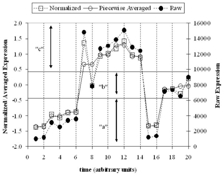
Schematic of converting a expression profile into a hash value.

The breakpoints can be obtained from tables of the Gaussian cumulative distribution function (CDF), or via eq. 3 by solving for x, where z is the number of breakpoints, n is an index variable in the range of 1 to z, and erf is the error function.

$$\frac{n}{z-1}=\frac{1}{2}[1+\text{erf}(\frac{x}{\sqrt{2}}\left)\right]$$ (3)

The overall process of converting the signal into its symbolic representation is shown in Fig. 1.

The final part of the process involves converting the symbolic representation into an integer. This is accomplished by treating the sequence as a base N number, where N is the number of breakpoints. By then converting to a base 10 number as in eq. 4, we obtain an integer (h), where, if two genes hash to the same integer, they have similar expression profiles, where c is symbol obtained from eq. 3, w is the length of the sequence, and a is the size of the alphabet.

$$h=1+{\sum }_{j=1}^w[\text{ord}(c_j)-1]a^{w-j}.$$ (4)

Characterization of the Transcriptional State of the System and Extraction of the Most Informative Expression Patterns

After the conversion of the gene expression pattern into a set of motifs (hash values), we then evaluated which of these motifs were required to capture the nonrandom progression of the entire expression profile over time. This was done by first defining a concept we term the transcriptional state. This allows for the construction of a metric that characterizes the inherent dynamic state of the system that allows monitoring of the dynamic progression and evolution of the system. Such a quantifiable metric allows us to evaluate just how informative the selected subset of probe sets is. The basic premise is that there exists a core set of genes whose transcriptional machinery is most affected by the stimulus. Furthermore, this core set of genes represents the fundamental response of the system and thus accounts for its essential dynamics. To characterize the dynamic state of the system, we treat the expression levels of each probe set as variables that follow a specific, albeit unknown, distribution. The drug will alter these distributions over time to perturb the underlying transcriptional machinery of each gene, quantified by the corresponding amounts of mRNA. Given such perturbations, it would be expected that, over time, the distribution of expression values of the most informative subsets of genes would show greater deviations from both the Gaussian and the baseline (control) expression levels.

To quantify this observation, the Kolmogorov-Smirnov (K-S) test, is employed. The K-S test is applicable to unbinned distributions that are functions of a single independent variable. The list of data points over time can then be easily converted to an unbiased estimator of the cumulative distribution function of the probability distribution from which the expression values were drawn. Therefore, truly informative subsets of genes are the subsets that have the ability to capture significant deviations from the base distribution. The K-S test is a simple yet effective way of comparing two distributions, and it has had many applications, such as the estimation of diversity in chemical libraries (Rassokhin and Agrafiotis, 2000).

The K-S is defined as the maximum absolute difference between two cumulative distribution functions. For each time point, we estimate a CDF of the expression values, after a double normalization step. The first normalization of the expression profiles sets the range of all profiles to the same scale. The second normalization is performed so that distributions of the same family are lumped, whereas distributions of different families are quantified as different. For example, this will lump all normal distributions no matter what the parameter together, whereas a normal parameter and an exponential parameter would be classified as different. By doing so, we can ascertain whether different mechanistic factors are affecting the distribution of gene expressions at the different time points.

The base distribution is the corresponding CDF before administration of the drug. The K-S statistic (D) is thus defined as were n is the number of genes in a given population and i is the index of a particular gene and its associated position on the CDF:

$$D=\underset{1\le i\le n}{max}|F(Y_i)-F(Y_i(0))|$$ (5)

where F(Y_i(0)) is the cumulative distribution of the expression values at time t = 0. This statistic allows a metric that defines the magnitude of the difference between two distributions to be computed. Because the data are presented as a time series, at each time point a value for the K-S statistic is obtained. Therefore, the overall metric becomes as follows:

$$D=\underset{t}{max}\underset{1\le i\le n}{max}|F[Y_i(t)]-F[Y_i(0)]|$$ (6)

The application of the K-S test over time allows us to quantify just how much the CDF of a particular subset of genes deviates from the corresponding CDF at time t = 0 (control). The most sensitive subset exhibits the largest deviations from the control. Once the subset is specified, then it can be characterized based on its corresponding D value. The individual genes in a subset are then defined by the previously described hashing procedure. We have implemented a simple greedy algorithm that selects peaks based on their ability to maximize the deviation from the control distribution of expression values. The basic steps of the algorithm are presented in Table 1.

TABLE 1.

Basic steps of the algorithm that selects peaks based on their ability to maximize the deviation from the control distribution of expression values

k = 0,S(k) = Ø,D(k) = − ∞, max = − ∞ k = k + 1 h* = arg max N(h), N(h) = number of genes with corresponding hash value h G(k) = {gi; hash(gi) = h*}, the subset of genes that hash to h Evaluate F(Ygi(t)); t = 0, K, T; gi ϵ Σ Evaluate $$D(k)=\underset{t}{max}\underset{g\text{i}\in \Sigma }{max}|F[Y_{g\text{i}}(t)]-F[Y_{g\text{i}}(0)]|$$ If D(k) > max Max = D(k); F = k; Go to (ii) until all peaks have been added For a = 1 to F Select Σ = S(a – 1) U G(a)

The iteration count, k, corresponds to the number of peaks that are incorporated at each step; S(k) is the set of hash values that have been considered up to iteration k; N(h) is the number of genes probe sets that have been assigned to a particular hash value h; h* is the motif values that is most populated at each iteration; G(k) is the subset of genes g_i, that have hashed to h, whereas S is the cumulative set of genes included at each iteration. D(k) is the K-S statistic evaluated at iteration k, and it is calculated using the set S of genes. Once a peak and its corresponding S probe sets have been included, then the corresponding hash value is eliminated so that it is not considered again. The search is performed in the space of peaks, as opposed to individual probe sets, and peaks (along with the corresponding probe sets) are added, provided that a clear deviation from the control state is observed.

Results

Major Expression Patterns

Figure 2 depicts the distribution of motif values for rat liver gene expression after dosing with MPL. The algorithm isolated 529 of a total of 8799 probes into 12 clusters. The justification for this selection is given in Fig. 3. The first 12 clusters produced the most evident deviation from baseline of the transcriptional state. Although there exist other overpopulated clusters that are not included, we do not dispute the fact that these genes may be significant, nor do we claim that the selected genes are more biologically significant. Instead, what we claim is that given factors such as noise, the selected genes are the genes from which the global dynamics are most visible. This is significant because it is from the global dynamics as PK/PD response model can be constructed. We use the signal-to-noise ratio (SNR) defined as SNR = 20*log₁₀ [μ(g)]/[σ(g)] as a measure of signal quality. The SNR measures signal quality by comparing the scale of the mean versus the scale of the standard deviation. The μ represents the mean of the signal, and σ represents the S.D. of this reported value (Greshock et al., 2007). The value is reported in decibels, which is the log transformation of the value. The greater the mean is in relation to the variance, the greater the SNR. Given the logarithmic formulation of the SNR, a signal in which the S.D. is the same as the mean would have an SNR of 0, whereas if the S.D. was smaller than the mean, the SNR would be positive, and negative otherwise. The genes selected via the algorithm have a minimal SNR of 2 db and a mean SNR of 16 db, with the majority of the genes (67%) having an SNR of above 12 db. This means that in all cases, the signals selected, the mean values were significantly greater than the variance. SNR was chosen as a method for quantifying quality because of it offers a rough measure as to how effective signal processing methods are at extracting the intrinsic dynamics.

Fig. 2.

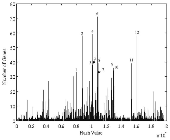
Motif distribution of our data. Motifs 1 to 12 were selected as relevant motifs.

Fig. 3.

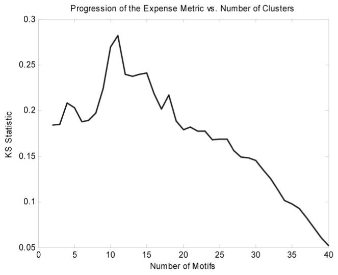
Expense metric as a function of number of clusters added. After the critical number of clusters has been added, the metric starts to decline. Although there may be information present in additional clusters, their addition degrades the overall quality of the metric.

Figure 4 provides the 12 expression versus time profiles for all of the genes in each cluster. They exhibit clear characteristics of early up- or down-regulation, and the expression levels in these patterns return to baseline with time. It is evident that the hash-based clustering has yielded groups of genes with highly correlated activity. The selection of these clusters does not preclude other genes and clusters from having a biological role. Rather, these 12 clusters represent the majority of responses that comprise what we deem to be the intrinsic system dynamics.

Fig. 4.

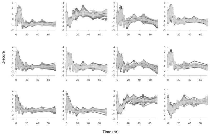
The z-score expression of all the clustered genes.

Characterization of the Transcriptional State of the System

Figure 5 depicts the deviation from the t = 0 distribution for the informative probe sets belonging to the 12 primary motifs selected by the algorithm. The temporal evolution of the transcriptional state and the plot of the objective function over time (Fig. 6) show that the initial deviation is followed by an eventual return to the initial state. These 12 peaks reveal the minimum number of expression signatures (not individual genes) whose presence is critical for reproducing the dominant transcriptional response of the system. The K-S statistic reflects the overall dynamics, with a large deviation from the baseline before hour 10, and then a return to the initial state. This is in agreement with an acute pharmacodynamic response in which the responses to the single bolus dose of drug occur early, and then the responses are reduced over time as the drug is cleared from the system.

Fig. 5.

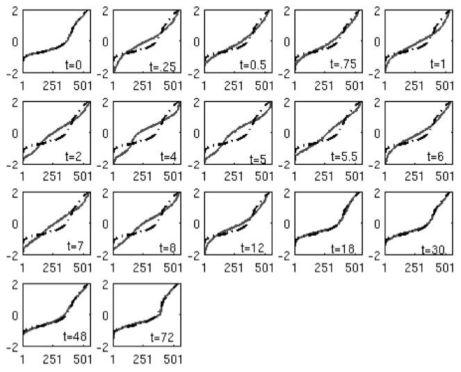
Comparison between the transcriptional state between time n versus time 0. Dashed line is the transcriptional state of time 0, and solid line is the transcriptional state at time n.

Fig. 6.

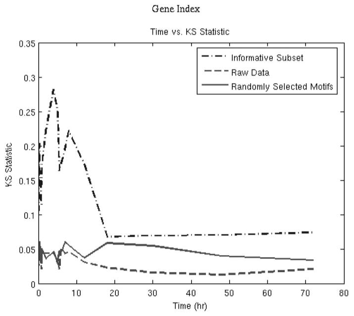
Comparison between the objective functions between the entire set of genes, 529 informative probes, and 529 randomly selected probes.

Dynamic Response Model

Aside from being useful as a metric for the selection of informative genes, the K-S statistic itself offers valuable information as to the overall response of the system to the single bolus dose of MPL. Using the K-S statistic rather than individual genes for model creation allows us to treat the system as an aggregate and to obtain a time constant of drug activity rather than time constants of specific genes. This negates the need to first identify a candidate gene as was done in the original approach. From the K-S plot in Fig. 6, we hypothesized that the overall drug response could be modeled as a closed loop linear time invariant (LTI) model. This does not mean that the underlying corticosteroid response is linear, just that for this single drug dose, the system can be approximated as a linear mass-action system. We acknowledge the fact that there exist significant nonlinearities in the system as evidenced by the fact that the overall corticosteroid response shows a tolerance mechanism during repeated dosing (Sun et al., 1998). This violates the linearity properties of the LTI model. This simplification was based upon the fact that the overall shape of the damped response was very similar to the original response. This means that the response can be modeled either as a nonlinear system or a piecewise linear system by taking the nonlinear portions of the model and piecewise linearizing them. To obtain the primary components of the system, we have elected to do the latter. This simplification is then used to provide specific intuitions about the response of the system. This model can later be modified to include specific nonlinear components such as receptor saturation and receptor ligand interactions that would then allow us to model behavior such as the dose-dependent nonlinear response and the aspect of tolerance. This approach is something dissimilar to the mechanistic-based modeling proposed previously in which intuitions about the system is used to create a comprehensive model (Jin et al., 2003), in that we seek to create a framework response, and then we incorporate additional factors such as nonlinearities when faced with additional data. The addition of these other factors essentially allow us to hypothesize the behavior of important control elements in the system, rather than requiring their knowledge a priori, and this represents the difference between a hypothesis-driven approach versus a data-driven discovery approach.

A LTI model satisfies two properties. First, it has a non-time-dependent response. This means that there is no implicit time definition, and so the modeling equation is defined as f(x(t)), where x(t) is the input, rather than f(x(t), t). This property is supported by use of ADX rats to eliminate the circadian effects of endogenous corticosterone. The second is that the system must reflect the principle of superposition. This means that f(x(t) + y(t)) = f(x(t)) + f(y(t)), in which both x(t) and y(t) are separate inputs. The primary attraction of this method is that it greatly simplifies the overall construction of the model.

The LTI formulation allows for the use of the convolution integral to determine the response of the system from an input eq. 7. The use of the convolution integral is attractive because it allows the system to be described in the Laplace domain eq. 8, which allows for identification of mathematical representations of physical factors or elements that amplify or dampen the input response f(x).

$$f\times g={\int }_0^{t}f(\tau )g(t-\tau )d\tau$$ (7)

The gross schematic of a closed loop LTI model is shown in Fig. 7. The model consists of a gain term k(s) and a feedback term g(s). The feedback term relates the current state of the system to a future state, and it does not strictly imply the presence of the gene product activating a pathway that will then deactivate it. The simplest mechanism that could function as this feedback term would be a reservoir that couples the synthesis and degradation rates of mRNA.

Fig. 7.

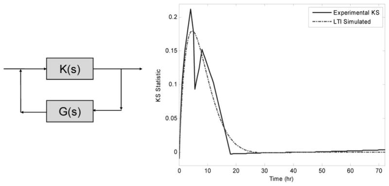
Proposed gross model and simulated drug activity. The feedback term (s + b)(s + c) associated with G(S) implies a two-compartment system with an associated degradation term. K(s) was found to be constant.

Nominally, an LTI system is a set of differential equations (Oppenheim et al., 1997). In the simplest case, a single input/single output model, the differential equation can be written as in eq. 8, where (m) and (n) represent the degree of differentiation (first, second, third derivative):

$${\sum }_{n=0}^p{a}_n{y}^{(n)}={\sum }_{m=0}^q{b}_m{x}^{(m)}$$ (8)

The Laplace transformation is defined in eq. 9. It is closely related to a Fourier transform, and it is often used in electrical engineering for systems identification (Franklin et al., 2002):

$$L[f(t)](s)={\int }_0^{\infty }f(t)e^{-\text{st}}dt$$ (9)

The advantages of the Laplace representations are 2-fold. The prediction of the response to other inputs such as chronic drug infusion can be achieved through simple algebraic manipulation. In addition, the Laplace domain differential equation has distinct physical meaning, and it can provide insight as to the underlying mechanisms that govern the observed response.

The conversion of a first-order differential equation into the Laplace domain is given in eq. 10:

$$\begin{array}{c}{y}^{\prime }+ay=x\\ L[y^{\prime }+ay]=L[x]\\ Y(s)=\frac{X(s)}{(s+a)}\end{array}$$ (10)

This generalized form has the corresponding Laplace transform given in eq. 11, which in our case has the constraint where m > n:

$$Y(s)=\frac{\Pi (s+a_n)}{\Pi (s+b_m)}$$ (11)

This additional constraint imposes stability upon the system that is not universally required, but in the context of a biological responses to corticosteroids it is reasonable. An unstable response would indicate a changing of state after the drug has been cleared from the system. This could result in death as the organism would be unable to recover homeostasis. In eq. 11, we can represent the system as the quotient of two polynomials. The polynomial is then factored with the terms in the numerator representing the “zeros” of the equation and the terms in the denominator representing the “poles” of the equation. The factorized terms in the numerators function as inductors, whereas in the denominator function as capacitors. The biological analog of a capacitor is a compartment that accumulates the buildup of the input signal or mRNA, and the biological analog of an inductor is the inertia of the signal. For example, in the circulatory system, the mass of the fluid being displaced can act as an inductive element (Ferrari et al., 2003).

The feedback as described in this system does not necessarily correspond to the biological notion of feedback. It only requires that the rate of change, i.e., dx/dt, be dependent upon X or the amount already present in the system. This can be handled via the more familiar indirect response models where the amount of the signal or mRNA directly affects the sensitivity to the signal or the production of mRNA. However, it could also be modeled as a mass action system in which the rate of loss is dependent upon concentrations already present through changes in either degradation or production rates. However, at this point, we do not consider the mechanism for feedback, but only establish that there is a mechanism.

Part of the reason behind SLINGSHOTS was the extraction of the global dynamic. Figure 7 integrates the expression profiles of different genes. Using the Laplace formulation, we fitted the global dynamic to the general form given in eq. 11, while minimizing the overall number of terms. This was accomplished via the LSIM command in MATLAB (Mathworks Inc., Natick, MA), which takes the Laplace representation and is able to simulate an impulse response that leads to the response observed in Fig. 7. It was found that the data could have been fitted via eq. 12, an equation with no terms in the numerator except for a constant scaling factor which can be thought of as a constant amplification factor of the mRNA signal, and two terms in the denominator indicates the need for two capacitance elements:

$$Y(s)=\frac{k}{(s+a_0)(s+a_1)}$$ (12)

The first capacitance element (a₀) is the circulation that acts as a compartment that can store a portion of corticosteroid dose. The second capacitance element (a₁) includes the cells where the signal alters the production of mRNA, thereby having an indirect rather than direct effect. This reflects the original hypothesis that the activity of corticosteroids is mediated via drug from plasma interacting with tissue receptors.

Given the agreement between this model and those derived previously (Dayneka et al., 1993), we think that the global dynamic obtained via our K-S statistic acts as a good surrogate for the global activity of a population of genes, thereby obviating the need to specifically identify genes that respond to corticosteroids through a priori knowledge. The primary advantage of using both the K-S statistic and the pole-placement model for modeling identification is that it is a data driven approach, and it is independent of researcher bias. It does this without any loss in generality, as seen in the agreement between the gross mechanistic aspects of the indirect response models (Dayneka et al., 1993) and the mechanical underpinnings of our model.

Functional Dynamics

To examine the functional dynamics of the system, we conducted an extensive literature review of all affected genes. The genes were separated into different functional categories that spanned multiple clusters, and the hierarchical clustering and visualization gene tree approach (Eisen et al., 1998) was applied as modified by the GeneSpring software (Agilent Technologies, Palo Alto, CA). We used this algorithm to construct a dendrogram of genes with similar patterns based on the Pearson correlations. A negative aspect of this tool is the assumption that the points in the time series are equally spaced. Notwithstanding this drawback, gene trees provide an excellent method of visualizing the data set. It was necessary to first transform the data so that the values for all probe sets were within the same range. Values for each probe set on each chip were expressed as a ratio of the mean of the four control values for that gene, which we refer to as “normalized intensity.” Thus, the average of each probe set has a value of 1.0 at zero time and either increases, decreases, or remains unchanged relative to controls over the time series. Yellow in the graph represents an expression ratio around 1, or no change. The color progressing toward red indicates a normalized value greater than 1, or up-regulation, and the color toward blue indicates a value less than 1, or down-regulation from control levels. Figure 8, A to L, provide the dendograms for the 12 functional categories (Other and EST were excluded). These figures provide an overview of the effects of MPL on the overall functional dynamics of the liver. For example, the dominant red color in Fig. 8A demonstrates that the general effect on transcription and translation is to enhance the expression of the particular genes. It is interesting to note that there is limited down-regulation of genes seen as a blue band at the bottom. Notable among these genes is retinoid X receptor, which is strongly down-regulated. This is probably related to alteration of lipid metabolism seen in Fig. 8K. In contrast, Fig. 8B shows that there is both significant enhancement and down-regulation of genes involved in signaling. Figure 8C shows that the dominant effect of MPL is down-regulation of genes involved in small-molecule metabolism. The interesting exceptions of glutamine synthetase and ornithine decarboxylase in cluster 1 along with argininosuccinate lyase and carbonic anhydrase in cluster 4 are involved in disposal of the ammonia produced by gluconeo-genesis from amino acid carbon. These figures also demonstrate that the majority of the effects of MPL are finished by12 h, although some effects on immune-related genes (Fig. 8E) and mitochondrial genes (Fig. 8J) persist well beyond this time.

Fig. 8.

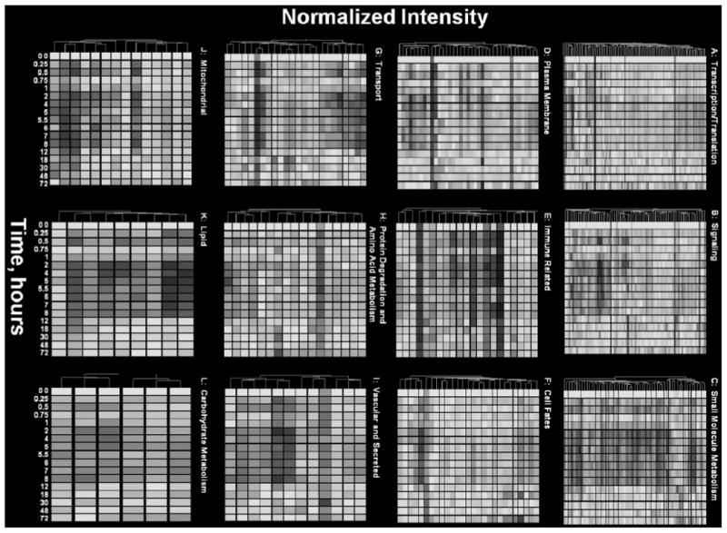
Temporal gene expression data of genes in 12 key functional categories.

Discussion

The primary mechanism of action of corticosteroids is alteration of the expression of genes. In contrast to drugs that have direct actions where there is a relationship between the drug concentration at the effect site and magnitude of the response, corticosteroids have indirect effects on gene turnover that persist long after the drug has dissipated. Most of the extracted profiles have similar dynamics as those found in the previous analysis, which consists of an initial deviation from the baseline followed by a relaxation back to the initial state (Jin et al., 2003).

This experiment was designed such that the single dose of MPL initiated molecular events in time that continued until the complex system returned to its initial equilibrium state. The pattern recognition approach within the context of the rich time series design allowed us to observe the overall dynamics of the system as it is perturbed and re-equilibrates. Our method identifies the dominant motifs of this dynamic process, and the genes that comprise these profiles. This approach is different from the commonly used “clustering algorithms” such as K-means or SOM where some similarity measurement (e.g., correlation or Euclidian distance) is used to collect genes into a predetermined number of similarity groups. The present approach seeks in an unsupervised, “top down” manner to identify the dominant motifs governing the dynamics of the system. The use of this system dynamics approach allowed us to both characterize the behavior of this complex system and to parse into groups the contributing elements of the system.

One of the difficulties with creating a PK/PD model from individual genes or clusters is that it is difficult to tease out the interplay between the different clusters. In an ideal situation, representative genes would respond only to the input of corticosteroids. This is problematic for two reasons. First, it is difficult to determine whether the gene responds only to MPL. Methods such as computational prediction of transcription factor binding sites are not sufficiently sensitive to fully identify the possible regulators of a given gene, and even techniques such as ChipChip experiments cannot identify which of the possible regulators are active in a given study. Second, the derivative effects of corticosteroids such as the elevation of circulating glucose may have effects on the overall system, and such secondary changes may not be captured by a single gene.

In a previous study, we generalized a representative gene to identify genes with similar patterns (Almon et al., 2007). Models were developed describing responses of these sets of genes (Jin et al., 2003). This approach allowed for the incorporation of secondary effects and the identification of time-lagged responses, but it was not able to account for complexities such as the possibility that each of the genes may interact with each other. Our previous corticosteroid models were simplified as one dose of MPL was given and different interactions were not considered. The models generated in such a manner were not always applicable for a chronic infusion regimen (Almon et al., 2007). Attempts have been made to add back into the model the links in the form of other biosignals and transduction steps and further work will be needed to identify and quantify the transcriptional links that tie together the disparate subsystems.

Creating models from the overall dynamics of the system represents a level of abstraction that bridges the gap between the simplicity of a single gene model and more complete model(s) derived from multiple genes. It allows for the creation of models that do not require the explicit identification of interactions between different genes, while still exhibiting the salient properties of the system. In this case, we posited a central necessity of having a two-component model that agrees with the general properties found in the indirect response models (Dayneka et al., 1993). Building a model from the global dynamics helps provide initial intuitions about the system. It is more complete than single gene models because it allows for a composite response that can come from multiple genes. It lumps the different expression profiles into a single dynamic. In addition, the global response provides an alternative but complimentary view of the response dynamics to drug administration rather than looking at individual genes or systems that are affected. Instead of considering the individual gene time courses, one considers the degree, the extent, and how long the drug has a tangible effect upon the overall system. This representation provides an overall context for the development of more complex models for those genes of special interest.

The intersection of the 216 probes extracted in the original analysis and the 529 probes extracted via the new method, there was an interaction of only 56 probe sets. Although this may seem like a small amount, using analysis of variance on the data set, with a p < 1.13 × 10⁻⁴, yielded 267 genes with an intersection of only 36 genes. A majority of the genes that intersected between the two data sets were found in clusters 1 and 6 in the original analysis and with a single gene found in cluster 4. These correspond to the up-regulated, down-regulated cluster, and one cluster that originally was termed “biphasic” in which there was an initial down-regulation and then an up-regulation above the initial baseline level before returning to the final steady state. In this analysis, we will not be differentiating the biphasic response as a separate mechanism because it can be reconstructed via the standard two-pole LTI model as easily as the other systematic profiles, and it suggests the existence of a complex pole. Physically, the LTI model can be implemented as a delay in the system either through inertial means such as differences in diffusion rates or in the case of the CS models, the implementation of a lag term in which there is an intermediate gene that is transcribed, which later activates another gene as denoted by intermediate biosignal (BS) in the original CS model (Jin et al., 2003).

Two of the clusters that were not found in our analysis correspond to clusters 2 and 5, which are sparsely populated and therefore do not seem to be part of any significant coordinated event. However, of greater concern is cluster 3 in the original analysis, which again shows a systematic overshoot profile but was not selected via our SLINGSHOTS algorithm. This may be due to the greater variability in the cluster due perhaps to intermediate signals that are not consistent between the genes as evidenced by the large difference in the k_{d_BS} in the genes of that cluster when associated with the fifth generation model, showing that they have different intermediate signals; therefore, they are not direct effects of corticosteroid on mRNA expression levels but rather secondary effects that may still be important. The breakdown of cluster coherence as the corticosteroid response progresses through multiple layers of the cascade is something that can be addressed with parameters with less granularity such as increasing the windows size from two time points to three time points. However, this loss of coherence weakens the concept of coexpression implying coregulation (Wolfe et al., 2005). Therefore, we think that the SLINGSHOTS algorithm represents one of the many steps needed to fully decipher complex transcriptional mechanisms; therefore, it does not negate the value of the previous analysis.

The original motivation for re-examining the extensive gene array data were to determine whether a more comprehensive set of genes affected by MPL could be selected. In this formulation, we identified 529 probes as opposed to the 192 that had been found initially. The high correlation of the genes selected lends confidence in the clusters. From these genes, we have isolated many major components that are responsible for the effects of corticosteroids, such as transcriptional signaling, small-molecule metabolism, and genes responsible for controlling metabolic shift changes.

Most importantly, we have identified the global dynamics of the system and we have proposed a relatively simple model that can be used as the basis to model the dominant PK/PD responses of the liver to MPL. Although this model is less complete than the previously devised PK/PD models, it has the primary response feature of the model, namely, turnover of mRNA. Although the interplay between the different genes has not been identified or quantified, the current model explains the general response pattern. The identification and quantification of the systems that are responding as part of this global response will be a logical next step. In essence, we have created a framework within which additional PK/PD models for drug responses can be developed. The overall value of this algorithm is not so much its ability to select genes, but rather its selection of elementary response profiles and to describe the global response dynamics of the system.

Abbreviations

MPL

methylprednisolone

PK/PD

pharmacokinetic/pharmacodynamic

ADX

adrenalectomized

CDF

cumulative distribution function

K-S

Kolmogorov-Smirnov

SNR

signal-to-noise ratio

LTI

linear time invariant

CS

corticosteroid

BS

intermediate biosignal

References

- Almon RR, Dubois DC, Jusko WJ. A microarray analysis of the temporal response of liver to methylprednisolone: a comparative analysis of two dosing regimens. Endocrinology. 2007;148:2209–2225. doi: 10.1210/en.2006-0790. [DOI] [PMC free article] [PubMed] [Google Scholar]
- Chikanza IC. Mechanisms of corticosteroid resistance in rheumatoid arthritis: a putative role for the corticosteroid receptor beta isoform. Ann N Y Acad Sci. 2002;966:39–48. doi: 10.1111/j.1749-6632.2002.tb04200.x. [DOI] [PubMed] [Google Scholar]
- Cronstein BN, Kimmel SC, Levin RI, Martiniuk F, Weissmann G. A mechanism for the antiinflammatory effects of corticosteroids: the glucocorticoid receptor regulates leukocyte adhesion to endothelial cells and expression of endo-thelial-leukocyte adhesion molecule 1 and intercellular adhesion molecule 1. Proc Natl Acad Sci U S A. 1992;89:9991–9995. doi: 10.1073/pnas.89.21.9991. [DOI] [PMC free article] [PubMed] [Google Scholar]
- Dayneka NL, Garg V, Jusko WJ. Comparison of four basic models of indirect pharmacodynamic responses. J Pharmacokinet Biopharm. 1993;21:457–478. doi: 10.1007/BF01061691. [DOI] [PMC free article] [PubMed] [Google Scholar]
- Eisen MB, Spellman PT, Brown PO, Botstein D. Cluster analysis and display of genome-wide expression patterns. Proc Natl Acad Sci U S A. 1998;95:14863–14868. doi: 10.1073/pnas.95.25.14863. [DOI] [PMC free article] [PubMed] [Google Scholar]
- Ernst J, Bar-Joseph Z. STEM: a tool for the analysis of short time series gene expression data. BMC Bioinformatics. 2006;7:191. doi: 10.1186/1471-2105-7-191. [DOI] [PMC free article] [PubMed] [Google Scholar]
- Ferrari G, Kozarski M, De Lazzari C, Gorczynska K, Mimmo R, Guaragno M, Tosti G, Darowski M. Modelling of cardiovascular system: development of a hybrid (numerical-physical) model. Int J Artif Organs. 2003;26:1104–1114. doi: 10.1177/039139880302601208. [DOI] [PubMed] [Google Scholar]
- Franklin GF, Powell JD, Emami-Naeini A. Feedback Control of Dynamic Systems. Prentice Hall; Upper Saddle River, NJ: 2002. [Google Scholar]
- Greshock J, Feng B, Nogueira C, Ivanova E, Perna I, Nathanson K, Protopopov A, Weber BL, Chin L. A comparison of DNA copy number profiling platforms. Cancer Res. 2007;67:10173–10180. doi: 10.1158/0008-5472.CAN-07-2102. [DOI] [PubMed] [Google Scholar]
- Heyer LJ, Kruglyak S, Yooseph S. Exploring expression data: identification and analysis of coexpressed genes. Genome Res. 1999;9:1106–1115. doi: 10.1101/gr.9.11.1106. [DOI] [PMC free article] [PubMed] [Google Scholar]
- Indyk P, Motwani R, Raghavan P, Vempala S. Locality-preserving hashing in multidimensional spaces. Proceedings of the Twenty-Ninth Annual ACM Symposium on Theory of Computing; 1997 May 4–6; El Paso, TX. 1997. pp. 618–625. Association of Computing Machinery. [Google Scholar]
- Jin JY, Almon RR, DuBois DC, Jusko WJ. Modeling of corticosteroid pharmacogenomics in rat liver using gene microarrays. J Pharmacol Exp Ther. 2003;307:93–109. doi: 10.1124/jpet.103.053256. [DOI] [PubMed] [Google Scholar]
- Lin J, Keogh E, Lonardi S, Chiu B. A symbolic representation of time series, with implication for streaming algorithms. 8th ACM SIGMOD Workshop on Research Issues in Data Mining and Knowledge Discovery; 2003 June 13; San Diego, CA. 2003. pp. 2–11. [Google Scholar]
- Millenaar FF, Okyere J, May ST, van Zanten M, Voesenek LA, Peeters AJ. How to decide? Different methods of calculating gene expression from short oligo-nucleotide array data will give different results. BMC Bioinformatics. 2006;7:137. doi: 10.1186/1471-2105-7-137. [DOI] [PMC free article] [PubMed] [Google Scholar]
- Oishi K, Amagai N, Shirai H, Kadota K, Ohkura N, Ishida N. Genome-wide expression analysis reveals 100 adrenal gland-dependent circadian genes in the mouse liver. DNA Res. 2005;12:191–202. doi: 10.1093/dnares/dsi003. [DOI] [PubMed] [Google Scholar]
- Oppenheim AV, Willsky AS, Nawab SH. Signals & Systems. Prentice Hall; Upper Saddle River, NJ: 1997. [Google Scholar]
- Rassokhin DN, Agrafiotis DK. Kolmogorov-Smirnov statistic and its application in library design. J Mol Graph Model. 2000;18:368–382. doi: 10.1016/s1093-3263(00)00063-2. [DOI] [PubMed] [Google Scholar]
- Sun YN, DuBois DC, Almon RR, Pyszczynski NA, Jusko WJ. Dose-dependence and repeated-dose studies for receptor/gene-mediated pharmacodynamics of methylprednisolone on glucocorticoid receptor down-regulation and tyrosine aminotransferase induction in rat liver. J Pharmacokinet Biopharm. 1998;26:619–648. doi: 10.1023/a:1020746822634. [DOI] [PubMed] [Google Scholar]
- Sun YN, McKay LI, DuBois DC, Jusko WJ, Almon RR. Pharmacokinetic/pharmacodynamic models for corticosteroid receptor down-regulation and glutamine synthetase induction in rat skeletal muscle by a receptor/gene-mediated mechanism. J Pharmacol Exp Ther. 1999;288:720–728. [PubMed] [Google Scholar]
- Tilstone C. DNA microarrays: vital statistics. Nature. 2003;424:610–612. doi: 10.1038/424610a. [DOI] [PubMed] [Google Scholar]
- Wolfe CJ, Kohane IS, Butte AJ. Systematic survey reveals general applicability of “guilt-by-association” within gene coexpression networks. BMC Bioinformatics. 2005;6:227. doi: 10.1186/1471-2105-6-227. [DOI] [PMC free article] [PubMed] [Google Scholar]
- Yang E, Maguire T, Yarmush ML, Berthiaume F, Androulakis IP. Bioinformatics analysis of the early inflammatory response in a rat thermal injury model. BMC Bioinformatics. 2007;8:10. doi: 10.1186/1471-2105-8-10. [DOI] [PMC free article] [PubMed] [Google Scholar]