

Abstract
Advanced mathematical models have the potential to capture the complex metabolic and physiological processes that result in energy expenditure (EE). Study objective is to apply quantile regression (QR) to predict EE and determine quantile-dependent variation in covariate effects in nonobese and obese children. First, QR models will be developed to predict minute-by-minute awake EE at different quantile levels based on heart rate (HR) and physical activity (PA) accelerometry counts, and child characteristics of age, sex, weight, and height. Second, the QR models will be used to evaluate the covariate effects of weight, PA, and HR across the conditional EE distribution. QR and ordinary least squares (OLS) regressions are estimated in 109 children, aged 5–18 yr. QR modeling of EE outperformed OLS regression for both nonobese and obese populations. Average prediction errors for QR compared with OLS were not only smaller at the median τ = 0.5 (18.6 vs. 21.4%), but also substantially smaller at the tails of the distribution (10.2 vs. 39.2% at τ = 0.1 and 8.7 vs. 19.8% at τ = 0.9). Covariate effects of weight, PA, and HR on EE for the nonobese and obese children differed across quantiles (P < 0.05). The associations (linear and quadratic) between PA and HR with EE were stronger for the obese than nonobese population (P < 0.05). In conclusion, QR provided more accurate predictions of EE compared with conventional OLS regression, especially at the tails of the distribution, and revealed substantially different covariate effects of weight, PA, and HR on EE in nonobese and obese children.
Keywords: quantile regression, energy expenditure, obesity, childhood, heart rate, physical activity, accelerometry
understanding the intrinsic factors influencing energy expenditure (EE) is fundamental to understanding human energetics. Although the impact of intrinsic factors, such as age, sex, body mass, and composition on EE, has been thoroughly studied, prediction models in this field of research focus on the mean effect or central tendency, even though the effects at different levels of EE could be substantially different. In this article, quantile regression (QR) models will be introduced for the first time to predict EE and explore intrinsic factors affecting EE across the entire distribution. Elucidating the effect of intrinsic factors apart from the central tendency may enhance our knowledge of the energetics, for instance, investigating successful energy regulation in nonobese and dysregulation of energy balance in obese individuals.
For conceptual purposes, EE is partitioned into basal metabolism, thermogenesis, and physical activity (PA). Basal metabolism represents the energy needed to sustain the metabolic activities of cells and tissues, plus the energy to maintain blood circulation and respiration. Thermogenesis augments basal metabolism in response to stimuli unassociated with muscular activity, such as food ingestion and cold and heat exposure. PA may be defined broadly as all bodily actions produced by the contraction of skeletal muscle that increase EE above basal level (2). Body mass is the single largest factor influencing not only basal metabolism, but also PA. Corrected for body mass, the standard error for prediction of basal metabolism is on the order of ±7–9% in children (15). However, energy expended in PA is volitional and represents the most variable intra- and interindividual component of EE. Throughout the day, PA is the prime determinant of the variation observed in EE for an individual. For these reasons, we will focus this article on the prediction of and covariate effects on EE during the awake period of the day.
Room respiration calorimetry can be used to assess the effects of the intrinsic variables on energy metabolism. Room respiratory calorimeters are small rooms in which a person may reside comfortably for long periods while oxygen consumption and carbon dioxide production are monitored continuously under controlled environmental conditions. Ancillary variables, such as body movement and heart rate (HR) that reflect PA, can be measured simultaneously with small electronic devices, such as accelerometers and HR monitors.
Ordinary least squares (OLS) linear regression models have been used conventionally to estimate individual variation in EE and the impact of influential factors. Alternatively, the QR model (9), a nonparametric statistical methodology, can be used to examine how the covariates influence the location, scale, and shape of the entire response distribution (7, 12, 20). QR estimates the conditional median or other quantiles of the outcome variable, given the values of the predictor variables. Each conditional quantile denotes the value of the response variable, in our case EE, below which the proportion of the population with the given values of the predictor variables is equal to that quantile. One advantage of QR, relative to the OLS regression, is that the QR estimates are more robust against outliers (9, 14) and automatically adapted to the data heterogeneity (9). The QR model does not assume any parametric form of the error distribution. Different from the OLS model, which focuses on the estimation of mean and variance, the QR model can be fitted at a family of quantile levels. These QR estimates at different quantile levels provide an alternative way to characterize the statistical dispersion of the data, without specifying an underlying parametric model. A typical QR model usually assumes that one or a family of conditional quantiles of the outcome variable can be expressed as a function of the predictors, e.g., a linear combination of the predictors. But this function also is allowed to take different parameter values or even different forms at different quantile levels once the monotonicity over quantiles is preserved. For example, the QR model allows that certain predictors may influence the outcome variable only at quantiles, i.e., τ > 0.9.
An important feature of the QR model is that it focuses on how the predictors or covariates influence the outcome variable at several selected quantile levels of interest. Such influence can be different in nature and magnitude at different quantile levels (1, 16). In that sense, QR provides different measures on the covariate effects of the central tendency and tails trends and thereby provides a comprehensive analysis of the relationship between variables. Compared with the other conventional nonparametric approaches, like splines-based regression methods, QR can directly target the quantiles of interest without modeling the whole conditional distribution and also provide a direct model interpretation on the effect of each explanatory variable.
The primary objective of this study is to apply QR modeling to predict EE and determine the effect of intrinsic, explanatory variables at different quantile levels of EE in children and adolescents. First, QR models will be developed to predict minute-by-minute awake EE at different quantile levels based on HR and PA, and child characteristics of age, sex, weight, and height in nonobese and obese populations. Second, the QR models will be used to evaluate the covariate effects of weight, PA, and HR on minute-by-minute across the conditional EE distribution.
MATERIALS AND METHODS
Study design.
A cross-sectional study was designed to develop and validate equations for the prediction of EE from accelerometry and HR monitoring in 109 children and adolescents, ages 5–18 yr, using 24-h room respiration calorimetry. The inclusion criteria required the children to be healthy and free from any medical condition that would limit participation in PA. The Institutional Review Board for Human Subject Research for Baylor College of Medicine and Affiliated Hospitals approved the protocol. All parents gave written, informed consent to participate in this study.
Subjects.
Subjects (n = 109) were Hispanic, African American, and Caucasian children, aged 5–18 y. Forty-eight children (44%) were classified as obese by the Center for Disease Control and Prevention growth charts (11).
Methods.
The physiological measurements have been described in detail elsewhere (21) and only briefly here. Body weight to the nearest 0.1 kg was measured with a digital balance, and height to the nearest 1 mm was measured with a stadiometer. Body mass index was calculated as weight/height2 (kg/m2), with obesity defined as ≥95th percentile for body mass index (11).
During the 24-h calorimetry, continuous measurements of EE, HR, and activity were collected in a room respiration calorimeter (21). The 24-h calorimetry protocol reflected the wide range of physical activities in which children typically engage, from sleeping to moderate-vigorous physical activities, to capture the physiological relationships between EE and age, sex, weight, height, HR, and PA. During the daytime, the children completed a series of activities with “free time” and meal time between planned activities. The specific activities included working on a computer, watching television, watching a movie, assembling a floor puzzle, playing video games, walking on the treadmill at 2.5 mph and 3.1 or 3.7 mph, slow jogging on the treadmill at 3.1–4.3 mph, playing active videos, performing aerobic exercises, dancing, and jogging/running on the treadmill at 3.7–6.2 mph.
EE computed using the Weir equation (19) was averaged at 1-min intervals. The Actiheart device (CamNtech, Cambridge, UK) was used to monitor HR and PA. Actiheart is composed of an ECG signal processor and an uniaxial accelerometer built from a cantilevered rectangular piezo-electric bimorph plate and seismic mass, which is sensitive to movement in the vertical plane. Actiheart data were collapsed into 60-s intervals and aligned with the minute-by-minute EE data. HR data were filtered with an upper cutoff of 240 beats/min and a lower cutoff set at 10 beats/min below the subject's average sleeping HR. To utilize the equations in this paper, the activity counts from the CamNtech unit should be multiplied by 5/6 to achieve the same value as the MiniMitter unit (per CamNtech).
QR modeling.
In this article, we introduce a new analytic approach, QR, to predict the minute-by-minute EE from PA, HR, and individual characteristics of age, sex, weight, and height. To apply the QR model to predict the minute-by-minute EE based on HR, PA, and other potential predictors, let yij denote the minute-by-minute EE measures on the i-th individual at consecutive time points j. We consider the following QR model:
| model 1 |
where Qτ(yij) is the τ-th conditional quantile of yij, i.e., P[yij ≤ Qτ(yij)|xij, zi] = τ; β(τ) are the regression quantiles associated with xij (HR and PA related covariates); and γ(τ) includes the intercept parameter and the regression quantiles associated with subject-specific covariates, such as age and sex. Essentially, model 1 assumes that the τ-th conditional quantile of EE can be expressed via a linear function of the observed covariates x and z. Note that x and z may include a quadratic or even higher order term of the covariate.
In the usual QR, the regression quantile estimates of model 1 are defined as
i.e., is the minimizer of the above objective function, and ar gmin is argument of the minimum. The above regression quantile estimates can be easily solved through standard optimization techniques (3, 10, 13). The resultant estimates are asymptotically normal (9). More details related to the computation issues and theoretical properties of the regression quantile estimates can be referred to Koenker and He and Shao (6, 8). For any specific quantile level τ, the regression quantile estimates can be used to estimate the τ-th conditional quantile of the outcome variable y, i.e., . For example, in model 1, the estimates the EE level, below which there are approximately 90% of population with the same values of covariates x and z.
Different from any mean regression model (e.g., OLS regression) which focuses on how various covariates influence the mean of the outcome, model 1 investigates how the covariates influence a family of quantile levels of the conditional distribution of the outcome variable. It has been recognized that the estimates of covariate effects on the conditional mean of EE were not necessarily indicative of the size and nature of these effects on the upper and lower tails of the EE distribution. By looking at any family of quantile levels (e.g., τ = 0.1, 0.25, 0.5, 0.75, 0.9), the QR model in model 1 provides an estimate of the conditional quantile functions of EE at those selected quantile levels and, therefore, provides a more comprehensive picture on how the covariates influence the entire distribution (i.e., location and shape) of the minute-by-minute EE. The distinguishing feature of model 1 is that the regression coefficients β(τ) and γ(τ) may differ across quantile levels τ. This property is practically meaningful in the sense that it can distinguish the covariate effects of HR, PA, and those subject-specific covariates on the EE between the upper/lower tails and the central trends. Another advantage of model 1 is that it does not assume any parametric form of the error distribution and allows the error distribution to depend on a certain set of covariates. If the regression quantile estimates substantially differ across quantile levels, it indicates that the error distribution is not homoscedastic, and the location shift interpretation of the covariate effect is implausible. Therefore, compared with any other parametric model, model 1 is more flexible in adapting to the heterogeneity of EE. The model 1 at τ = 0.5 provides a robust alternative to the corresponding OLS regression model. The prediction can be used to predict the cutoff value of the EE with any specification of the confidence level τ.
RESULTS
Development of QR models.
As a result of our modeling process, the final model as in model 1 utilizes the following set of covariates: xij contains PA, PA2, PAlag1, PAlag2, HR, HR2, HRlag1, HRlag2, HRlead1, and HRlead2; zi includes the intercept age, age2, sex, weight, and height. In this work, we consider data from the awake period of the 24-h calorimeter protocol only. We fit QR models for the two subpopulations, nonobese and obese, respectively.
The QR model in model 1 with τ = 0.5 can be viewed as a robust alternative to the corresponding OLS regression estimates. Therefore, we can also use the QR model with τ = 0.5 to predict the minute-by-minute EE, i.e., use . We obtained the prediction equations from the QR model and the OLS model for nonobese and obese populations, respectively, with self-centered and standardized covariates age, age2, weight, height, PA, PAlag1, PAlag2, HR, HRlag1, HRlag2, HRlead1, and HRlead2 and the corresponding square terms age2, PA2, and HR2.
1) Nonobese populations
| 1 |
| 2 |
2) Obese populations
| 3 |
| 4 |
where EE is in kcal/min; weight is in kg; height in cm; gender is coded as male = 0, female = 1; HR is in beats/min; and PA is in counts/min.
We used fivefold cross validation to evaluate the prediction accuracy of the QR and OLS models. We fitted the QR model with τ = 0.5 using the fitting data and used the remaining fold as testing data. We used the prediction error calculated by avg as a numeric criterion to evaluate the prediction accuracy of the predictions from the QR model and those from the corresponding OLS regression model. The results are given in Table 1, from which we can clearly see the QR model obtains smaller prediction errors for both the nonobese and obese populations, compared with the OLS predictions. Similar results that the QR model obtains smaller prediction errors are observed when the absolute prediction error calculated by |yi − ŷi| is used to evaluate the prediction accuracy.
Table 1.
Average prediction errors for τ from the QR and the OLS models for energy expenditure in the nonobese and obese populations
| Nonobese | Obese | |
|---|---|---|
| QR, % | 17.7 (16.3, 16.6, 19.8, 18.2, 17.4) | 19.6 (18.2, 22.2, 16.1, 21.2, 20.3) |
| OLS, % | 20.7 (17.9, 19.9, 23.3, 21.2, 21.2) | 22.0 (18.9, 26.2, 18.3, 24.8, 22.0) |
QR, quantile regression; OLS, ordinary least squares. Nos. in parentheses are the prediction errors in the fivefold cross validation presented separately.
To evaluate QR at the tails of the distribution of EE, the quantile prediction equations at τ = 0.1, 0.9 for the obese and nonobese populations with self-centered and standardized continuous covariates are listed below.
1) Nonobese populations
| 5 |
| 6 |
2) Obese populations
| 7 |
| 8 |
To evaluate the prediction accuracy of the QR models at the tails of the distribution, we compared the predicted τ-th conditional quantile of EE using the QR model constructed from the fitting data, with the actual τ-th conditional quantile of the EE in the testing data. Because the actual τ-th conditional quantile of the EE in the testing data is unknown, we approximate it by using the estimated τ-th quantile of EE from the QR model applied on the testing data directly. In the fivefold cross validation, we fitted the QR model at τ to the fitting data first and then applied the fitted QR model to the testing data, denoting ŷi as the model predictions from the testing data. We also fitted the QR model at τ to the testing data directly and estimated the τ-th conditional quantile of EE in the testing data, denoted as ỹi. We use the prediction error calculated by avg(|ŷi − ỹi|/ỹi) as a numeric criterion to evaluate the accuracy of the predictions from the QR model. For comparison, we also calculated the prediction error of the OLS model, by taking ŷOLS(τ) = ŷOLS + qτ σ̂, where ŷOLS is the OLS prediction of the conditional mean, qτ is the τ-th quantile of the standard normal distribution, and σ̂ is the estimated standard error from the OLS model. The results are given in Table 2, from which we can clearly see the QR model obtains smaller prediction errors for both the nonobese and obese populations, compared with the OLS predictions at the two tail quantiles 0.1 and 0.9. Similar results that the QR model obtains smaller prediction errors are observed when the absolute prediction error calculated by |yi − ŷi| is used to evaluate the prediction accuracy.
Table 2.
Average prediction errors for τ from the QR and the OLS models for energy expenditure in the nonobese and obese populations
| Nonobese | Obese | |
|---|---|---|
| τ = 0.1 | ||
| QR, % | 9.2 (11.5, 4.2, 11.5, 7.8, 11.1) | 11.1 (13.2, 10.1, 8.8, 13.7, 9.6) |
| OLS, % | 39.0 (25.7, 35.9, 39.4, 34.0, 60.0) | 39.3 (47.0, 33.0, 34.3, 46.7, 35.4) |
| τ = 0.9 | ||
| QR, % | 7.6 (7.9, 5.1, 9.2, 9.6, 6.4) | 9.8 (11.6, 12.2, 9.0, 9.2, 6.9) |
| OLS, % | 18.8 (18.7, 19.7, 17.3, 16.9, 21.4) | 20.8 (12.9, 28.8, 21.2, 19.6, 21.5) |
Nos. in parentheses are the corresponding prediction errors for the fivefold cross validation presented separately.
An alternative way to evaluate the prediction accuracy of the QR model at the tails of the distribution is to compare the proportion of observed EE above the predicted τ-th quantile of EE, i.e., Q̂(τ)(y|x,z), for which a more accurate prediction means the proportion should be close to its nominal level 1 − τ. For comparison, we compared the predictions from the QR model with those from the OLS model. The OLS model at different quantiles differs only in the intercept parameter, i.e., the slope parameter for each covariate is assumed to be constant at all quantiles. In contrast to the OLS model, the QR model allows the slope parameter to differ across quantiles. Such different covariate effects can be critical for an accurate tail prediction. We report the prediction accuracy of QR and OLS at τ = 0.1, 0.9. The average proportions from the fivefold cross validation are summarized in Table 3. Compared with the OLS predictions, the average proportions of EE above the QR predictions are closer to the nominal levels 1 − τ, which indicates that the QR model produces a more accurate prediction at the low and high quantiles of the distribution.
Table 3.
Average proportions of the observed energy expenditure in the testing data that are above the predicted τ-th quantile of energy expenditure from the QR and OLS models for the fivefold cross validation
| τ = 0.1 |
τ = 0.9 |
|||
|---|---|---|---|---|
| Nonobese | Obese | Nonobese | Obese | |
| QR, % | 89.6 | 86.5 | 11.4 | 11.4 |
| OLS, % | 94.3 | 94.6 | 6.2 | 6.3 |
Covariate effects of weight, PA, and HR across different quantile levels.
In this section, we demonstrate graphically how the covariate effects of weight, PA, and HR on EE may differ across quantiles by examining how the corresponding regression quantile coefficient estimates of these covariates based on their original scales change across τ, when adjusted by the other covariates. The 90% confidence bands of the resultant QR estimates also are presented. For reference, we provide the corresponding OLS estimate and its 90% confidence interval, which represents the mean covariate effect on EE. The coefficient estimates and the corresponding standard errors from the QR model at τ = 0.2, 0.5, 0.8 are listed in Table 4.
Table 4.
Coefficients estimates of weight, PA, PA2, HR, and HR2 at τ = 0.2, 0.5, 0.8 from the QR model for energy expenditure in the nonobese and obese populations
| Nonobese |
Obese |
|||||
|---|---|---|---|---|---|---|
| τ = 0.2 | τ = 0.5 | τ = 0.8 | τ = 0.2 | τ = 0.5 | τ = 0.8 | |
| Weight (e-02), kg | 1.28 (0.03) | 1.72 (0.03) | 2.13 (0.05) | 0.74 (0.02) | 1.03 (0.02) | 1.34 (0.03) |
| PA (e-03), counts/min | 1.77 (0.04) | 2.40 (0.05) | 2.92 (0.07) | 2.84 (0.10) | 3.88 (0.12) | 4.69 (0.15) |
| PA2 (e-06), counts min2 | −0.47 (0.01) | −0.63 (0.02) | −0.75 (0.03) | −1.09 (0.04) | −1.57 (0.05) | −1.87 (0.05) |
| HR (e-02), beats/min | −0.18 (0.09) | 0.01 (0.08) | 0.18 (0.13) | −0.93 (0.16) | −2.89 (0.23) | −3.08 (0.25) |
| HR2 (e-04), beats/min2 | 0.03 (0.05) | −0.13 (0.04) | −0.27 (0.06) | 0.41 (0.08) | 1.31 (0.12) | 1.45 (0.13) |
Nos. under each τ-th quantile are the units of the corresponding coefficient estimates. Nos. in parentheses are the corresponding SEs of the coefficient estimates. Coefficient estimates differed between the obese and nonobese population (with all P values <0.05). PA, physical activity; HR, heart rate.
Figure 1, A and B, shows an increasing trend of the covariate effect of weight as τ increases for both the nonobese and obese populations, respectively, which suggests that the covariate weight has more substantial positive effects on the upper quantiles of EE. The nonuniform covariate effect across τ also indicates that the error distribution depends on the covariate weight. Also, the association between weight and EE is generally stronger for the nonobese than the obese population. As indicated in Table 4, the coefficients for the association between weight and EE for the nonobese and obese populations differ significantly, with all P values < 0.05 based on a Wald-type test of the difference of the regression quantile coefficients of weight. The standard errors of the regression quantile estimates for PA, PA2, HR, and HR2 are usually larger for the obese than the nonobese population.
Fig. 1.
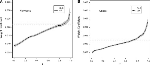
Regression quantile estimates of the covariate weight (vertical axis) against quantile levels of energy expenditure (EE) τ ∈ (0,1) (horizontal axis) for the nonobese (A) and obese populations (B). The solid line with solid circles represents the quantile regression (QR) estimates of weight for τ, ranging from 0.05 to 0.95, with the gray area as the corresponding 90% pointwise confidence band. The gray solid line is the corresponding ordinary least squares (OLS) estimate, and the two gray dotted lines provide its 90% confidence interval.
Figure 2, A–D, shows the covariate effects of PA and PA2 over quantile levels τ for the nonobese and obese populations, respectively. We made the following observations. 1) The covariate effects of PA and PA2 are nonuniform for the nonobese and obese populations, indicating that the error distribution depends on PA and PA2. For both subpopulations, PA has a more substantial effect on the upper tails of EE. 2) In general, the associations (linear and quadratic) between PA and EE are considerably stronger for the obese than the nonobese population (with all P values < 0.05). 3) The covariate effect of PA on EE changes more rapidly over τ for the obese population. The above observations are consistent with the numerical results listed in Table 4 for the coefficient estimates.
Fig. 2.

Regression quantile estimates of physical activity (PA; A and B) and PA2 (C and D) change against quantile levels of EE τ for the nonobese population (A and C) and for the obese population (B and D). The solid line with solid circles represents the QR estimates of weight for τ ranging from 0.05 to 0.95, with the gray area as the corresponding 90% pointwise confidence band. The gray solid line is the corresponding OLS estimate, and the two gray dotted lines provide its 90% confidence interval.
Figure 3, A–D, shows how the regression quantile estimates of HR and HR2 change over quantile levels τ for the nonobese and obese populations, respectively. We made the following observations. 1) The covariate effects of HR and HR2 are quite stable for the nonobese population, with a modest change in the upper tails, roughly τ > 0.6. For the obese population, the covariate effects of HR and HR2 change more substantially in the lower tails and are stable in the upper tails. 2) For the nonobese population, the covariate effect of HR is slightly stronger in the upper tails. For the obese population, the covariate effect of HR is significantly stronger in the upper tails of EE. 3) In general, the associations between HR, HR2, and EE are stronger for the obese than the nonobese population. 4) For the nonobese population, the OLS estimates, as indicated in Figure 3C, strongly suggest that effects of HR on EE are mainly linear with an insignificant quadratic effect. Instead, the QR estimates suggest that the quadratic effect of HR is significantly negative in the upper tails. For the obese population, both the OLS estimates and the QR estimates display a significant linear and quadratic effect of HR at most quantile levels. 5) In the upper tails, the QR estimates display a substantial positive quadratic effect for the obese population, in contrast to the nonobese population. The statistical significance of the comparison between nonobese and obese populations can be demonstrated with all P values < 0.05 based on the Wald-type test using the coefficient estimates and standard errors estimates listed in Table 4.
Fig. 3.

Regression quantile estimates of heart rate (HR; A and B) and HR2 (C and D) change against quantile levels of EE τ for the nonobese population (A and C) and for the obese population (B and D). The solid line with solid circles represents the QR estimates of weight for τ ranging from 0.05 to 0.95, with the gray area as the corresponding 90% pointwise confidence band. The gray solid line is the corresponding OLS estimate, and the two gray dotted lines provide its 90% confidence interval.
The QR model in model 1 is fitted at τ = 0.1, 0.25, 0.5, 0.75, 0.9 for the nonobese and obese populations, respectively. Table 5 represents the regression quantile estimates of PA, PA2, HR, and HR2 at those five quantile levels for the two subpopulations. As shown in Table 5, the effects of PA and HR on EE are different in size between the nonobese and obese populations. Such disparity is more substantial in the upper tails than the lower tails of the distribution.
Table 5.
Regression quantile estimates of PA, PA2, HR, and HR2 at τ = 0.1, 0.25, 0.5, 0.75, 0.9, for prediction of energy expenditure in the nonobese and obese populations
| τ = 0.1 |
τ = 0.25 |
τ = 0.5 |
τ = 0.75 |
τ = 0.9 |
||||||
|---|---|---|---|---|---|---|---|---|---|---|
| PA, | PA2 | PA | PA2 | PA | PA2 | PA | PA2 | PA | PA2 | |
| N-O | 1.57 e-03 | −4.20 e-07 | 1.88 e-03 | −5.06 e-07 | 2.40 e-03 | −6.34 e-07 | 2.87 e-03 | −7.21 e-07 | 3.09 e-03 | −7.60 e-07 |
| O | 2.42 e-03 | −9.39 e-07 | 3.04 e-03 | −11.81 e-07 | 3.89 e-03 | −15.72 e-07 | 4.42 e-03 | −17.55 e-07 | 5.35 e-03 | −20.86 e-07 |
| HR | HR2 | HR | HR2 | HR | HR2 | HR | HR2 | HR | HR2 | |
| N-O | −1.74 e-03 | 0.41 e-05 | −1.60 e-03 | 0.15 e-05 | 0.11 e-03 | −1.34 e-05 | 0.47 e-03 | 2.03 e-05 | 0.29 e-03 | −1.95 e-05 |
| O | −8.93 e-03 | 4.06 e-05 | −12.15 e-03 | 5.44 e-05 | −28.86 e-03 | 13.12 e-05 | −34.00 e-03 | 16.18 e-05 | −30.67 e-03 | 14.77 e-05 |
O, obese; N-O, nonobese. The regression quantile estimates are shown for PA and PA2, and HR and HR2.
Figure 4 represents the conditional quantile curves of EE against PA and HR at τ = 0.1, 0.25, 0.5, 0.75, 0.9 for the nonobese and obese population, respectively. To have a more explicit graphical representation, we transform the other covariates to be uncorrelated with the covariates of interest, i.e., PA and PA2 in the top two panels, HR and HR2 in the bottom two panels. As shown in Fig. 4, the conditional quantile curves have more disparity with larger values of PA and HR. As PA increases, EE changes at a slower rate for the nonobese than the obese population in both the upper and lower tails. For obese populations, with high PA, e.g., PA > 2,000 counts/min, EE actually decreases considerably faster as PA increases further. In our sample, there are few samples with PA > 2,500 counts/min, and the resultant QR estimates may be substantially influenced by those few outlying covariates. As HR increases, EE increases at a faster rate in the upper tails of the distribution and tends to be more convex in the upper tails than in the lower tails. EE shows more variation with higher HR for the obese than the nonobese population.
Fig. 4.

The fitted conditional quantile curves of EE against PA and HR for the nonobese and obese populations. In each panel, the five fitted quantile curves correspond to τ = 0.1, 0.25, 0.5, 0.75, 0.9, respectively, in the order that the lower curve corresponds to the lower quantile level.
DISCUSSION
For the first time, QR was applied for the prediction of EE and modeling of intrinsic, explanatory factors on EE across its entire distribution. Most EE models focus on predicting the conditional mean value of EE based on explanatory variables such as PA and HR and individual characteristics using OLS regression (5, 17, 18, 22). However, these models provide little information about the effects of the explanatory variables at different levels of EE which could be substantially different from the mean effect or central tendency. In this pediatric application, we demonstrated that the QR model resulted in smaller prediction errors for both nonobese and obese populations compared with the OLS predictions at the mean and also at the tails of the distribution. The covariate effects of weight, PA, and HR on EE for the nonobese and obese children differed substantially across quantiles, when adjusted by the other covariates.
QR modeling is a nonparametric approach for examining how the covariates influence the location, scale, and shape of the entire response distribution (8, 12, 20). The QR model does not assume any parametric form of the error distribution. Compared with OLS regression, QR estimates are more robust against outliers and automatically adapted to the data heterogeneity. More importantly, QR provides different measures of the covariate effects in the central tendency and tails trends, and such effects can be different in nature and magnitude at different quantile levels. By fitting QR at a family of quantile levels, we obtain a more comprehensive analysis of the relationship between variables. Different from the conventional nonparametric approaches like splines-based regression models, QR focuses directly on how the covariates influence the outcome variable at the selected quantile levels of interest, without modeling the whole conditional distribution.
QR outperformed the conventional OLS method for the prediction of EE across its entire distribution. As expected, the average prediction errors for the QR and OLS models at the tails of the distribution were much smaller for QR that OLS (10.2 vs. 39.2% at τ = 0.1 and 8.7 vs. 19.8% at τ = 0.9, respectively), but also smaller at the median τ = 0.5 (18.6 and 21.4%, respectively). We also evaluated the proportion of observed EE below or above the predicted τ-th quantile of EE at τ = 0.1, 0.9. Compared with the OLS predictions, the average proportions of EE from the QR predictions were closer to the expected values, indicating that the QR model produced a more accurate prediction at the lower and higher quantiles of the distribution.
QR also provides a robust, comprehensive understanding of the impact of covariates, such as weight, PA, and HR across the distribution of EE. The covariate effect of weight was larger in the nonobese than obese children, probably due to differences in body composition (4, 22). The obese children have a higher proportion of fat mass, which has a lower metabolic rate than fat-free mass. However, in both the nonobese and obese children, we found that weight has more substantial positive effects on the upper quantiles of EE. Both the linear and quadratic associations between PA and EE are stronger for the obese than the nonobese population. For a given value of accelerometer counts, the obese children have higher EE, controlling for the other covariates. The associations between HR and HR2 with EE are stronger for the obese than the nonobese population. The covariate effects of HR and HR2 are quite stable for the nonobese population, oscillating around zero, whereas they change more substantially in the lower tails and are stable in the upper tails for the obese population.
We have demonstrated the usefulness of the QR for prediction and modeling of EE in children. QR not only outperforms the conventional OLS method, but also enables us to properly handle the impact of explanatory covariates on EE when there is heterogeneity in the data. In this pediatric application, QR provided more accurate predictions of EE, especially at the tails of the distribution, and revealed substantially different covariate effects of weight, PA, and HR on EE in nonobese and obese children.
GRANTS
This project has been funded with federal funds from the United States Department of Agriculture/Agricultural Research Service under Cooperative Agreement no. 58-6250-0-008, and National Institute of Diabetes and Digestive and Kidney Diseases Grant R01 DK074387.
DISCLAIMER
The contents of this publication do not necessarily reflect the views or policies of the USDA, nor does mention of trade names, commercial products, or organizations imply endorsement by the U.S. Government.
DISCLOSURES
No conflicts of interest, financial or otherwise, are declared by the author(s).
AUTHOR CONTRIBUTIONS
Author contributions: Y.Y., A.L.A., M.R.P., F.A.V., and I.F.Z. analyzed data; Y.Y., A.L.A., N.F.B., and I.F.Z. interpreted results of experiments; Y.Y. prepared figures; Y.Y. and I.F.Z. drafted manuscript; Y.Y., A.L.A., M.R.P., F.A.V., N.F.B., and I.F.Z. edited and revised manuscript; Y.Y., A.L.A., M.R.P., F.A.V., N.F.B., and I.F.Z. approved final version of manuscript; A.L.A., M.R.P., F.A.V., and N.F.B. performed experiments; N.F.B. and I.F.Z. conception and design of research.
REFERENCES
- 1. Burgette LF, Reiter JP, Miranda ML. Explore quantile regression with many covariates: an application to adverse birth outcomes. Epidemiology 22: 859–866, 2011 [DOI] [PubMed] [Google Scholar]
- 2. Butte NF, Ekelund U, Westerterp KR. Assessing physical activity using wearable monitors: measures of physical activity. Med Sci Sports Exerc 44: S5–S12, 2012 [DOI] [PubMed] [Google Scholar]
- 3. Chen C, Wei Y. Computational issues for quantile regression. Indian J Statistics 67: 399–417, 2005 [Google Scholar]
- 4. Davies PSW, Cole TJ. The adjustment of measures of energy expenditure for body weight and body composition. Int J Body Compos Res 1: 45–50, 2003 [Google Scholar]
- 5. Goran MI. Measurement issues related to studies of childhood obesity: assessment of body composition, body fat distribution, physical activity, and food intake. Pediatrics 101: 505–518, 1998 [PubMed] [Google Scholar]
- 6. He X, Shao Q. A general Bahadur representation of M-estimators and its application to linear regression with nonstochastic designs. Ann Stat 24: 2608–2630, 1996 [Google Scholar]
- 7. Keming Y, Lu Z, Stander J. Quantile regression: applications and current research areas, statistical motivations and basic concepts of population and sample quantiles. Statistician 52: 331–350, 2003 [Google Scholar]
- 8. Koenker R. Quantile Regression. Cambridge, UK: Cambridge University Press, 2005 [Google Scholar]
- 9. Koenker R, Bassette G. Regresssion quantiles. Econometrica 46: 33–50, 1978 [Google Scholar]
- 10. Koenker R, d'Orey V. Computing regression quantiles. Statistician 36: 383–393, 1987 [Google Scholar]
- 11. Kuczmarski RJ, Ogden CL, Grummer-Strawn LM, Flegal KM, Guo SS, Wei R, Mei Z, Curtin LR, Roche AF, Johnson CL. CDC Growth Charts: United States. Adv Data 314: 1–27, 2000 [PubMed] [Google Scholar]
- 12. Marrie RA, Dawson NV, Garland A. Quantile regression and restricted cubic splines are useful for exploring relationships between continuous variables. J Clin Epidemiol 62: 511–517, 2009 [DOI] [PubMed] [Google Scholar]
- 13. Portnoy S, Koenker R. The Gaussian here and the Laplace tortoise: computation of square error vs. absolute-error estimates. Stat Sci 12: 279–300, 1997 [Google Scholar]
- 14. Rousseeuw PJ, Leroy AM. Robust Regression and Outlier Detection. New York: Wiley, 2005 [Google Scholar]
- 15. Schofield WN, Schofield C, James WPT. Basal metabolic rate-review and prediction, together with annotated bibliography of source material. Hum Nutr Clin Nutr 39C: 1–96, 1985 [PubMed] [Google Scholar]
- 16. Terry MB, Ferris JS, Tehranifar P, Wei Y, Flom JD. Birth weight, postnatal growth, and age at menarche. Am J Epidemiol 170: 72–79, 2009 [DOI] [PMC free article] [PubMed] [Google Scholar]
- 17. Trost SG, Pate RR, Sallis JF, Freedson PS, Taylor WC, Dowda M, Sirard J. Age and gender differences in objectively measured physical activity in youth. Med Sci Sports Exerc 34: 350–355, 2002 [DOI] [PubMed] [Google Scholar]
- 18. Trost SG, Sirard JR, Dowda M, Pfeiffer KA, Pate RR. Physical activity in overweight and nonoverweight preschool children. Int J Obes Relat Metab Disord 27: 834–839, 2003 [DOI] [PubMed] [Google Scholar]
- 19. Weir JB. New methods for calculating metabolic rate with special reference to protein metabolism. J Physiol 109: 1–9, 1949 [DOI] [PMC free article] [PubMed] [Google Scholar]
- 20. Willke RJ, Zheng Z, Subedi P, Althin R, Mullins CD. From concepts, theory, and evidence of heterogeneity of treatment effects to methodological approaches: a primer. BMC Med Res Methodol 12: 185, 2012 [DOI] [PMC free article] [PubMed] [Google Scholar]
- 21. Zakeri I, Adolph AL, Puyau MR, Vohra FA, Butte NF. Application of cross-sectional time series modeling for the prediction of energy expenditure from heart rate and accelerometry. J Appl Physiol 104: 1665–1673, 2008 [DOI] [PubMed] [Google Scholar]
- 22. Zakeri I, Puyau MR, Adolph AL, Vohra FA, Butte NF. Normalization of energy expenditure data for differences in body mass or composition in children and adolescents. J Nutr 136: 1371–1376, 2006 [DOI] [PubMed] [Google Scholar]