Signaling Events Initiated by Kappa Opioid Receptor Activation: Quantification and Immunocolocalization Using Phospho-Selective KOR, p38 MAPK, and K_IR 3.1 Antibodies

Abstract

Psychiatric disorders including anxiety, depression, and addiction are both precipitated and exacerbated by severe or chronic stress exposure. While acutely, stress responses are adaptive, repeated exposure to stress can dysregulate the brain in such a way as to predispose the organism to both physiological and mental illness. Understanding the neuronal chemicals, cell types, and circuits involved in both normal and pathological stress responses are essential in developing new therapeutics for psychiatric diseases. Varying degrees of stressor exposure cause the release of a constellation of chemicals, including neuropeptides such as dynorphin. Neuropeptidergic release can be very difficult to directly measure with adequate spatial and temporal resolution. Moreover, the downstream consequences following release and receptor binding are numerous and also difficult to measure with cellular resolution. Following repeated stressor exposure, dynorphin is released, binds to the kappa opioid receptor (KOR), and causes activation of KOR. Agonist-activated KOR becomes a substrate for G protein receptor kinase (GRK), which phosphorylates the Ser369 residue at the C-terminal tail of the receptor in the first step in the β-Arrestin-dependent desensitization cascade. Through the use of phospho-selective antibodies developed and validated in the laboratory, we have the tools, to assess with fine cellular resolution, the strength of behavioral stimulus required for release, time course of the release, and regional location of release. We have gone on to show that following KOR activation, both ERK 1/2 and p38 MAP kinase phosphorylation are increased through use of commercially available phospho-selective antibodies. Finally, we have identified that one effector of KOR/p38MAP kinase is K_IR 3.1 and have developed a phospho-selective antibody against the Y12 motif of this channel. Much like KOR and p38 MAP kinase, phosphorylation of this potassium channel increases following repeated stress. The following chapter discusses immunohistochemical and quantification methods used for phospho-selective antibodies used in various brain regions following behavioral manipulations.

1. Introduction

With the advent and implementation of fluorescently tagged viral constructs that can be used to selectively inhibit or activate specific brain regions (i.e., halorhodopsin and channelrhodopsin, respectively) or knock-down, rescue, or overexpress specific receptors, the ability to dissect the role of receptors in different neuronal circuits in affective and motivated behavior has advanced significantly. The use of phospho-selective antibodies in immunohistochemistry (IHC) assays can guide behavioral and physiological experiments and allows for a new level of selectivity beyond immediate early gene immunohistochemistry (e.g., c-fos IHC). In more recent years, the role of both ERK 1/2 and p38 MAPK in controlling cellular excitability, synaptic plasticity, de novo gene transcription, and behavior has been explored (3). In a study examining KOR-mediated conditioned place aversion (CPA) where the animal passively avoids a context paired with prior KOR agonist injection, it was shown that this CPA requires p38 MAPK activation. CPA (for review, see (4)) has been posited as a means to assess dysphoria-like behaviors. It has been demonstrated that in the same cell type, ERK 1/2 and p38 MAPK can be activated in parallel signaling pathways (5); one example is the case of stress-induced dynorphin release. Following KOR activation either with intraperitoneal injection of the exogenous agonist U50,488 or stress-induced dynorphin release, both phospho-ERK 1/2 immunoreactivity (IR) and phospho-p38 MAPK-IR are increased in the same cell types compared to saline-injected control animals (1, 2). While both ERK and p38 MAPK activities increase following stressor exposure in a KOR-dependent fashion, we found that p38 MAPK activation requires G-protein receptor kinase 3 (GRK-3) and β-Arrestin 2 recruitment, whereas ERK 1/2 activation occurs through a GRK-3-independent pathway (6). CPA caused by U50,488 requires phosphorylation of the Ser369 residue of KOR while KOR-dependent stress-induced analgesia does not (7). In contrast, ERK 1/2 activation still occurs in cells where this residue has been mutated to an alanine. Therefore, while both kinases are activated following repeated stress in similar cell types in the same regions, only p38 MAPK appears to play a role in KOR-mediated dysphoric-like behavior (1). This has provided critical insight into uncovering diverging roles for ERK 1/2 and p38 MAPK in mediating affective behavior and could not have been elucidated without the use of phospho-selective antibodies.

Both home-grown and commercially available phospho-selective antibodies are notoriously finicky and require extensive validation at a variety of stages of analysis. Most commonly, problems that occur include high background staining, nonselective immunoreactivity, and high degree of variability between subjects and even between adjacent slices. Methods can be developed to address each of these potential issues, and particular care must be taken to control the quality and consistency in the perfusion conditions, type of blocking buffer, number of washes, incubation time and temperature, and antibody concentration. Critical to producing valid and consistent results is care during imaging and quantification techniques. The technique has inherent subjectivity and therefore a certain degree of rigor and objectivity is required in the analysis.

2. Materials

2.1. Antibody Generation and Affinity Purification

2.1.1. Preparation of Antibody Affinity Column

Access to a UV spectrophotometer and high-speed centrifuge is required for several steps throughout the affinity purification process.

1. CNBr-activated Sepharose 4B.

2. 1 mM HCl.

3. 0.1 M NaHCO₃.

4. 0.1 M NaCl.

5. 1 M and 0.05 M Tris.

6. 0.1 M glycine.

7. 5 M MgCl₂.

8. 0.02% Sodium azide.

2.1.2. Affinity Purification

1. TBS/azide: 50 mM Tris 0.15 M NaCl, 0.02% sodium azide, pH to 7.4.

2. Serum containing antibody of interest.

3. 5 M MgCl₂.

4. 0.1 M glycine.

5. Centriprep-30.

2.1.3. Enzyme-Linked Immunosorbent Assay (ELISA) to Determine Antibody Production

1. PBS: 50 mM NaH₂PO₄ (monobasic), 6.9 g in 1 L 0.15 M NaCl, 8.766 g in 1 L and adjust pH to 7.4.

2. PBS-T (PBS/0.05% Tween-20): Add 250 μl Tween-20 to 500 ml of PBS.

3. 1% nonfat dried milk (NFdM) in PBS: Add 1 g of NFdM powder to 100 ml of PBS. Store at 4°C.

4. 1% BSA (bovine serum albumin) in PBS: Add 1 g BSA to 100 ml of PBS. Store at 4°C.

5. P-NP mix (makes 50 ml): In 40 ml of double distilled water: 10% diethanolamine (5 ml), 1 mg/ml p-nitrophenyl phosphate (50 mg), 100 μg/ml MgCl₂ (5 mg), 0.02% sodium azide (10 mg). pH solution to 9.8 and bring to volume. Store in a 50-ml conical tube wrapped tightly in foil and store at 4°C.

2.2. Perfusion Fixation

2.2.1. Solutions

1. 0.4 M Phosphate buffer (0.4 PB): In 1 L distilled water, add 10.5 g Sodium phosphate monobasic, 86.6 g Sodium phosphate dibasic. Filter and store at room temperature.

2. 0.1 M Phosphate buffer (0.1 PB): In 1 L add 250 ml 0.4 PB, 750 ml distilled water.

3. 4 % Paraformaldehyde: In a vented fume hood, add to a glass beaker 250 ml of 0.4 M PB, approximately 600 ml of distilled water, and 40 g of paraformaldehyde (PFA). Stir continuously on a heated magnetic stir plate bringing the temperature to 65°C. Once temperature is reached, reduce heat to 60°C and add 10 M NaOH dropwise until all the PFA has gone into solution. pH solution to 7.4. You may have to add a drop or two of HCl, but try to avoid this. Often, the sodium hydroxide takes a while to take effect. After a couple of drops, wait for about a minute to let the PFA go into solution before adding more. Following pH adjustment, filter solution using a funnel that is lined with standard filter paper (Grade 413). For immediate use (<1 month), store at 4°C. For more prolonged use, aliquot into 50 ml conical tubes and store at −80°C (see Note 1).

4. PBS (different from PBS above): In 1 L of 0.1 PB add 8.76 g NaCl.

5. 30% Sucrose: 30 g of sucrose into 100 ml of 0.1 PB.

2.2.2. Instruments

1. Peristaltic pump or 30–60 ml syringe. Peristaltic pumps allow for an initial flush of the blood vessels in the brain with PBS before perfusion with PFA and also are easier to control flow rate, but good fixations can be accomplished with a simple hand-held syringe.

2. Butterfly needle.

3. Sharp medium scissors.

4. Sharp fine scissors.

5. Hemostat.

6. Rongeurs.

7. Fine (#7) forceps.

8. Small spatula.

9. 15 ml conical tubes.

2.3. Immunohistochemistry and Tissue Sectioning

1. For tissue sectioning, prepare 0.1 PB with 0.1% sodium azide (make a 10% stock to be diluted 100-fold in the wells).

2. PBS.

3. Blocking buffer: In PBS, add 5% normal goat serum (NGS) (Vector), 0.3% Triton X-100 (Sigma) (see Note 2).

4. Primary antibody solution: In blocking buffer, add either one primary antibody or cocktail of primary antibodies. For primary phospho-antibodies, typical concentrations range from 1:25 to 1:300. For home-grown antibodies, the concentration is highly dependent on yield. For example, for phospho-KOR we use a range of concentrations from 1:25 (0.0132 μg/ml) to 1:100 (0.0089 μg/ml) for antibodies with yields of 0.33 to 0.89 μg protein/ml affinity purified stock concentration.

5. Secondary antibody solution: In blocking buffer, add either one secondary or cocktail of secondaries raised in the different host species. For example, AlexFluor 488, 555, 633, 647 secondary antibodies from Invitrogen are recommended to be used at a concentration of 1:1000. However, FITC, TRITC, Texas Red, Cy2, Cy3, and Cy5 are available from Invitrogen or Jackson Immunoresearch work well, too. These antibodies may require higher concentrations, for example FITC works best in our hands at 1:250.

2.4. Fluorescence and Confocal Microscopy Imaging

1. Superfrost Plus slides (for mouse brains use, 25 × 75 × 1 mm).

2. Coverslip glass (for slide size above, coverslip size should not exceed 24 × 50 mm).

3. Mounting media: There are several different types of mounting media on the market with different advantages. Vectashield (with and without 4’,6-diamidino-2-phenylindole, DAPI) (Vector) is rather inexpensive by volume. However, clear nail polish is often required and there is no antifade technology. ProLong Anti-fade mounting kit (Invitrogen) is more expensive by volume, but reduces fluorescence fading and becomes increasingly more congealed, preventing cover slips from sliding around as easily.

4. Clear nail polish.

2.5. Quantification

While Metamorph software (Molecular Devices, Sunnyvale, CA) allows for more sophisticated quantification of image intensities or cell counts, basic quantification can be achieved with Adobe Photoshop.

3. Methods

The initial validation of phospho-selective antibodies, KORp, and p-Y12-K_IR 3.1 developed in this laboratory included a combination of ELISA and immunocytochemistry techniques (8, 9). For ELISAs, different concentrations of antibody (0.005–10 μg/ml) were incubated overnight with separate wells coated by peptides (0.5 μg/ml) corresponding to approximately amino acids having the key residue phosphorylated or nonphosphorylated (8-10). Further validation can be obtained by transfecting DNA constructs in appropriate tissue culture cell lines (e.g., HEK 293, AtT 20, COS-7) to allow expression of the wild-type and mutant form of the protein of interest. For example, treatment of HEK 293 cells expressing KOR-GFP by U50,488 produced concentration-dependent agonist-induced internalization and increased KORp-IR, whereas parallel treatment with HEK cells transfected with KOR having Ser369 mutated to an alanine (KSA-GFP) failed to show agonist-induced internalization or increased KORp-IR. Similarly, untransfected HEK cells and pretreatment with KOR antagonists provided important specificity controls.

A similar approach was used to validate a phospho-K_IR 3.1 antibody designed to detect the phospho-tyrosine-12 residue in the cytosolic amino terminal domain of the channel (9). It had been shown previously that TrkB activation by BDNF can phosphorylate tyrosine residues on K_IR 3.1 to accelerate deactivation of the channel (11). ELISA confirmed that the antibody reacted more strongly with the phospho-peptide than the nonphosphopeptide (9). K_IR 3.1-IR was evident when transfected cells were stimulated with BDNF (9). While the exact methodological protocols are beyond the scope of this chapter, before one can move on to IHC, these validation measures must be conducted when generating a new phospho-antibody.

These in vitro validation methods are usually extended to standard Western blot analysis (9, 10). This stage of validation can be done using cell-culture homogenates treated with various pharmacological manipulations or from brain and/or spinal cord tissue homogenates from animals subjected to either pharmacologic or behavioral manipulation. For example, for further validation of the phospho-K_IR 3.1 antibody, Western blots were done using spinal cord tissue from animals that were subjected to sham surgery or partial sciatic nerve ligation (pSNL). Spinal cord tissue from either the ipsi- or contralateral side for each animal was acquired and homogenized, the contralateral side providing a within-animal control. Samples were blotted for either pY12-K_IR 3.1 or total K_IR 3.1. (First, one must ensure that the phosphoantibodies run at the appropriate weight and that there are no nonspecific bands. The intensities of the bands can be quantified using the Odyssey infrared imaging system (LI-COR Biosciences) and plotted as either fold change over experimental control or loading control (e.g., β-Actin) (9, 10)). As expected, there was no difference in total K_IR 3.1 between sham and pSNL-treated animals, nor between ipsi- and contralateral sides of the same animal. pY12-K_IR 3.1-IR was evident only in tissue from the ipsilateral spinal cord of the nerve-ligated subjects (9). This set of experiments not only validates the antibody, but acts as a good compliment to IHC.

Generally, these in vitro methods are used prior to in vivo analysis. Perfusing, sectioning, staining, and imaging brain slices using phospho-selective antibodies are not drastically different than many other staining protocols that look at the localization and amount of total protein across brain regions. However, these primary antibodies seem particularly sensitive to poor fixation and sectioning as well as variations in incubation time and temperature. The following description of our current protocols may be a very useful starting point for the individual optimization processes required for each new analysis.

3.1. Generation, Validation, and Affinity Purification of Phospho-Selective Antibodies

3.1.1. Antibody Generation

1. Indentify an amino acid sequence within the protein of interest containing a known phosphorylation site. A typical amino acid sequence length would be approximately 12–15 amino acids with an added N-terminal lysine that enables conjugation to the BSA and Sepharose column (12). Using the GenBank™ data base, ensures that the sequence chosen is unique, no other proteins have >50% homology or four identical amino acids in a row.

2. The phospho-peptide is conjugated to KLH and injected into rabbits. Again, contract commercial services are available. 500 μg of antigen peptide was combined with Complete Freund’s Adjuvant for initial inoculation, then animals received boost inoculations of 250 μg of antigen peptide on days 14, 21, 49, 56, and monthly thereafter. Bleeds (approximately 6–7 ml) are collected once a month (9).

3.1.2. Preparation of the Affinity Column

1. Weigh 1 g of CNBr-activation Sepharose 4B. Swell for 15 min in 1 mM HCl and transfer to a sintered glass funnel. Wash with 200 ml of 1 mM HCl, then wash with 20 ml of 0.1 M NaHCO₃.

2. Suspend 2–5 μmol peptide in 0.1 M NaHCO₃, 0.1 M NaCl, pH 8.3. If the peptides are not soluble in this buffer, dissolve in water or acid and then adjust pH to 8.3. Bring the final volume to 5 ml. Measure and record OD₂₈₀ (optical density) to check concentration.

3. Add peptide solution to Sepharose and incubate overnight at 4°C with mild rocking.

4. Add 0.55 ml of 1.0 M Tris, pH 8.0. Rotate for 2 h at room temperature.

5. Pour slurry into a 0.7 × 15-cm column. Collect flow-through and measure OD₂₈₀ to determine peptide-coupling efficacy.

6. Wash 3× with 15 ml of 0.05 M Tris, pH 7.4, 0.15 M NaCl, then 15 ml of 0.1 M glycine, pH 3.0, then 1.5 ml of 5 M MgCl₂, and finally 15 ml of 0.05 M Tris, 0.15 M NaCl, pH 7.4.

7. For storage, wash column with 0.05 M Tris, pH 7.4, 1.5 M NaCl + 0.02% sodium azide. Store at 4°C.

3.1.3. Affinity Purification of Antipeptide Antiserum

1. Wash column before use with 20 ml TBS/Az.

2. Add 3–4 ml of serum to column. Seal the top and bottom with parafilm and gently rotate for 72 h at 4°C.

3. Wash unbound material with 20 ml TBS/Az, taking care not to let the resin dry.

4. Elute antibody with 5 ml 5 M MgCl₂, collecting into the outer vessel of a Centriprep-30 containing 5 ml TBS/Az.

5. Concentrate antibody in Centriprep to ~1 ml by spinning 1,5000 × g for 20 min (use Beckman J6-B centrifuge, set to 4°C and speed = 2,300 rpm). Discard fluid in central vessel. Add 5 ml TBS/Az to concentrated antibody in outer vessel, mix, and concentrate again to ~1 ml. Repeat twice more, adding cold TBS/Az each time (final concentration MgCl₂: 20 mM, after four additions of TBS/Az).

6. Measure OD₂₈₀ of concentrated antibody. Using a standard containing a known concentration of protein (i.e., BSA), get an OD₂₈₀ reading that will be used as the conversion factor for assessing the antibody concentration. For example, 1 mg/ml may yield an OD₂₈₀ reading of 1.4. Thus, if you get a reading of 1.2 for the purified antibody, the yield would be 0.857 mg/ml.

7. Dilute concentrated antibody by about half with glycerol and store at −20°C.

8. Following affinity purification, regenerate column (allow each of these to drip through) with 30 ml TBS/Az, then 30 ml 0.1 M glycine, then 5 ml 5 M MgCl₂. Add 35 ml TBS/Az and cap the top and bottom of the column and wrap ends with parafilm. It may not be necessary to regenerate the column after every affinity purification.

3.1.4. ELISA to Determine Antibody Production

Adopted from the method of Karen DeJongh and Aaron Patillo. This protocol assumes tested antibodies were raised in rabbit; if not, be sure to match the IgG-AP Ab used in Step 7 to the species (see Note 3).

1. Coat 96-well plates with 50 μl per well of a 10-μg/ml peptide solution, prepared in PBS. Prepare 5 ml per plate to be coated. Incubate overnight at 4°C or for 4 h at room temperature. Remove peptide solution from well.

2. Block unbound sites with 50 μl 1% skim milk powder in PBS. Incubate for 2 h at 37°C or overnight at 4°C.

3. Wash wells 3× 150 μl PBS-T. Swirl and remove solution by aspiration each time.

4. Identify and prepare the antibody dilutions in PBS-T for each bleed as desired. It is useful to create a standard data entry form to record the results for each concentration and bleed.

5. In triplicate, add 50 μl of diluted antibody to wells. Leave the upper three wells of each plate empty to use as a blank (fill with 50 μl PBS-T alone). Incubate for 2 h at room temperature or overnight for 4°C.

6. Wash wells 3× with 150 μl of PBS-T.

7. Add 50 μl of a 1:3,000 dilution of alkaline phosphatase-conjugated anti-rabbit IgG in PBS/1% BSA to each well. Incubate for 2 h at room temperature or overnight at 4°C.

8. Wash wells 6× with 150 μl PBS-T.

9. Add 50 μl of 1 mg/ml P-NP mix to each well. Incubate for 30 min at room temperature, protected from light. (You can place the plate(s) inside a lab bench drawer.) Do NOT empty wells when complete.

10. Add 50 μl 2.5 M NaOH to terminate reaction.

11. Using a plate reader, promptly read absorbance at 410 nM.

12. The phospho-selective antibody should react severalfold more strongly to a phosphopeptide than an equivalent nonphosphorylated sequence.

3.2. Perfusion Fixation

The following instructions are for intracardiac perfusion of mice or rats. Phospho-selective antibodies appear to be particularly sensitive to the quality of perfusion and postfixation protocol (see Note 4).

1. Set up the perfusion area with tools, butterfly needle, 50-ml tube of PBS, and either 50-ml tube of PFA for mice or 250-ml container for rats.

2. 15-ml tubes containing 4% PFA should be labeled accordingly and set aside.

3. If you have access to a peristaltic pump, attach butterfly needle and accompanying tubing to the tubing of the peristaltic pump so that there is tight seal between the two; ensure there is no leaking. Wrap parafilm around the needle, only leaving about 0.5 mm of the needle exposed to ensure that the need does not puncture the underside of the heart. If using syringe, simply attach needle to syringe full of PFA and skip Step 4.

4. Run the pump so that the tubing fills with PBS to the point where PBS is coming out of the needle. Then, transfer the input end of the peristaltic pump’s tubing to the 4% PFA. If the pump has a three-way stop-cock mechanism, then simply switch the dial so that the PFA will now flow through the tubing when switched on again.

5. Anesthetize the animal with Nembutal or isoflurane and proceed only when the animal is unresponsive to painful stimuli (foot pinch).

6. Secure the arms with pins or tape onto whatever surface has been designated for perfusions.

7. Use a pair of large-to-medium sharp scissors, pinch the fur and muscle around the abdomen upward, and make a deep angled cut into the flesh through the abdominal muscle, exposing, but not damaging the liver.

8. Cut up each side of the animal from the original abdominal incision to right below the arm pits exposing the liver, intestines, and chest cavity.

9. Use the small sharp scissors and make a horizontal cut across the diaphragm exposing the heart and lungs.

10. Use a hemostat and clamp the sternum and roll the hemostat toward the head of the animal exposing the heart further.

    Some people prefer to reverse Steps 11 and 12. This is a matter of preference and personal comfort.

11. Use small sharp scissors and cut the right atrium. Dark oxygenated blood should come out.

12. Insert butterfly needle into the left ventricle making sure to insert the needle perpendicular to the heart and into the apex of the ventricle. This is to avoid puncturing the septum and spilling PFA into the right ventricle.

13. Begin perfusing using syringe or peristaltic pump. For the first 5–10 ml (50 ml for rats) of PFA, the perfusion should be running at a rate of approximately 3–5 ml/min. Following this, reduce speed to 2 ml/min and perfuse the animal with the remaining PFA.

14. Decapitate the animal and dissect out the brain and place the brain in 4% PFA in 15 ml conical tube.

15. Following the perfusion, postfixate for anywhere from 1 to 12 h depending on the perfusion quality (more time for bad perfusions). Then, transfer the brains to 30% sucrose and incubate at 4°C until brain has sunk to the bottom of the tube.

3.3. Brain Sectioning

There are several different sectioning devices on the market from floor-standing cryostats to counter-top microtomes. Counter-top microtomes work well for free floating sections that are ≥30 μm. Thinner sections should be made using a cryostat and should be thaw-mounted on superfrost plus slides. The use of the above-mentioned phospho-selective antibodies has only been tested on free floating sections. It is not known if they are effective on thaw-mounted tissue sections. The following instructions are for counter-top microtomes.

1. Fill the cavity surrounding the mounting stage with dry ice that has been smashed into fine powder and wait until frost accumulates around the outside of the stage.

2. Remove brain from 15 ml conical tube. For coronal sectioning, cut off the brainstem and small portion of the cerebellum to create a flat surface. For sagittal sections, cut down the midline. Horizontal slices should not need any tissue blocking.

3. Using a transfer pipette, take the 30% sucrose solution and drip the solution onto the frozen stage until an appropriately sized bed layer forms. Do not let the solution freeze all the way before placing the brain on the stage with forceps. For coronal sections, the olfactory bulbs should be facing up. For sagittal sections, the most lateral temporal lobe should be facing up. For horizontal sections, either the most dorsal or ventral side up should work and should depend on regions of interest.

4. Drip more sucrose solution around the brain, waiting intermittently for each layer to freeze. Tissue-Tek ® OCT compound should also work and logistically is better to use if using a cryostat; however, we have not tested the efficacy of the antibodies following sectioning in OCT. (In the case of cryostat, create the bed layer of OCT on the removable circular block and mount the brain. Once the brain is affixed to the cryostat block, surround the tissue in OCT compound and quickly return to the cryostat to freeze. You may find that freezing the brain directly in dry ice before mounting on the cryostat block is more effective. However, this may affect the phospho-staining and cell morphology adversely).

5. Once the brain is surrounded in frozen sucrose solution, take a 50-ml conical tube that has had the closed end cut off and place over the brain. Then, take the fine dry ice powder and with a spoon pour it over the brain and wait for 45–60 s.

6. Remove tube and dust off dry ice exposing the frozen brain.

7. Using sharp disposable or reusable blades, begin sectioning brain. It is useful to moisten the blade with 0.1 PB to ensure smooth sectioning. If you still notice shredding of the tissue, place your finger on top of the tissue for 1 s. With these methods, the brain should not be too cold or the tissue will not section evenly.

8. Place sections into wells containing 0.1 PB with 0.1 % sodium azide and store at 4°C until you are ready to use slices. If you are interested in a singular brain region, then it is perfectly fine to section and confine the brain according to regions of interest. However, if you are interested in studying the entire brain, then the brain should be sectioned serially, placing one slice in well #1-X and then starting back at 1 such that each well contains a “representative brain.” Consult your mouse or rat atlas. Given a certain region of interest and thickness of section, you can calculate how many wells to use to ensure that each well contains approximately the same number of slices through the rostro-caudal axis of region.

3.4. Immunohistochemistry

For information regarding immunocytochemistry with these antibodies, please refer to:

1. In a set of 12 well plates, fill each well with PBS and select at least three representative sections along the rostro-caudal axis for each brain region of interest for each treatment group. There are plastic baskets with mesh at the bottom that are designed to fit in 12-well plates. However, these can be easily crafted using cell-culture baskets. It is highly recommended that you use these baskets rather than placing the sections directly into the wells and using a fine paint brush to transfer the sections from well to well. This avoids damaging the tissue (see Note 5).

   A common mistake is to overcrowd the sections. For robust antibodies that are used as cell-type markers such as NeuN or GAD67, this is not as large a problem. However, for phospho-selective antibodies, it is important that each section gets similar penetration. Therefore, select 3–6 sections per well depending on the size of the brain section. Each well may contain a sample of one brain region or if you wish to include a more complete representation of a single brain region, you may need to use 2–3 wells. Given the number of treatment groups, you may have to run your experiment in batches. This is fine as long as one conducts parallel staining of matching brain regions for each treatment group (e.g., Batch #1 Hippocampus from Treatment groups X–Z). Managing 4—6 12-well plates is approximately the upper limit. Depending on your question, it may not be possible to process sections from more than one subject per treatment group. This is not a problem as long as each treatment group is represented. While one would like to think that the staining should not differ from round to round, the reality is that it most definitely can vary. For each round of staining, the imaging will also be collected in parallel (see Subheading 3.5). The quantification averages either the intensity or cell counts from at least three sections from one animal to create a single N (see Subheading 3.6). Therefore, each batch will ultimately create a single N for each treatment group (if one animal per treatment group was used in a round of staining) and the representative images should be selected based on the mean intensity or cell count for each group.

2. Once the sections from each subject are selected, place sections in the first well (each column should be reserved for one set of sections from one subject) into the plastic basket. Make sure that at least 2 ml of PBS are in each well and sufficiently covering the sections.

3. Sections should be washed in PBS 3× 10 min with mild agitation on a shaker, transferring the basket containing the sections to the second and then the third well every 10 min. Make sure to remove excess PBS from previous well by gently touching the basket to the side of the well.

4. During the washes, prepare the blocking buffer.

5. Aspirate off the PBS from the first well.

6. Pipette 1 ml of blocking buffer into each well. Remove basket from third wash and touch a Kim® wipe to the bottom of the basket removing excess PBS and place the basket into the blocking buffer.

7. Once the basket is in the well with the blocking buffer, add an additional 1 ml of blocking buffer to each well.

8. Block for 1 h with mild agitation. During this time, prepare cocktail of primary antibodies making sure that each primary has been raised in a different host animal.

9. Both home-grown and commercial phospho-selective antibodies can be precious and expensive. To reduce the volume necessary for each set of sections, primary antibody staining can be done in 1.7 ml Eppendorf® tubes. For each set of sections, use 500 μl of blocking buffer containing primary antibody. Prepare one stock of primary antibody solution (e.g., for four Eppendorf ® tubes, prepare 2 ml of stock solution) than aliquot 500 μl of the solution into each carefully labeled Eppendorf ® tube.

10. Following the blocking step, place sections into their respective Eppendorf ® tubes containing the primary antibody solution with a fine paint brush. Phospho-selective antibodies often need at least 36 h of incubation at room temperature or 48–72 h of incubation at 4°C with mild agitation. Phospho-p38 MAPK and phospho-ERK 1/2 antibodies work in both conditions. Incubating for longer duration at 4°C appears to reduce background. Every 12–24 h, gently rotate each tube upside down and then place back into holder in upright position. KORp and pY12-K_IR 3.1 antibodies are typically incubated for 72 h at 4°C. If you notice uneven staining on a given section or across sections from the same set, you can also use a 24-well plate (no baskets) using a similar volume for each well that is used for the Eppendorf ® tubes (see Note 6).

11. The use of cell markers (e.g., TPH for serotonin, TH for dopamine/norepinephrine, GAD 67 for GABA, vGLUT1,2,3, for glutamate, GFAP for astrocytes, NeuN for neurons, etc.) is extremely useful for indentifying the colocalization of activated proteins to specific cell types (see Figs. 1 and 2). Most of these markers are very robust, often are mouse monoclonal antibodies (although some are raised in both rabbit and mouse such as GFAP and GAD) and work well in several different incubation conditions including those described above.

12. Most affinity-purified antibodies are raised in rabbit, while commercially available antibodies such as phospho-p38 MAPK are available in both mouse and rabbit hosts. Thus, it is possible to colocalize phospho-p38 MAPK with a home-grown antibody such as KORp as shown in Fig. 2. However, to assess the pattern of staining in a brain region of a subject for two rabbit polyclonal antibodies, one must take alternating serial sections from a brain region for staining of the two antibodies, respectively (Fig. 1).

13. For cell count or intensity quantification against total or non-phosphorylated protein, the antibodies for phosphorylated and nonphosphorylated protein must be raised in different host species in order to colabel the same tissue. If this is not possible, a ratio of intensities or cell counts can be constructed between activated and nonactivated regions present on the same section.

14. Following primary antibody incubation, fill 12-well plates (it is okay to use the same plates from Step 1 that have been rinsed and dried) with PBS.

15. Remove sections from their respective tubes and place into baskets in the first well containing PBS. Wash at least 3 × 10 min with mild agitation just as in Step 3. If you are noticing high levels of background staining, it may be necessary to increase this washing step to 4–6 × 10 min.

16. During this wash, prepare secondary antibody solution. If you are using natural goat serum, ensure that your secondary antibodies are goat antibodies (i.e., they should read goat anti-mouse or goat anti-rabbit) (see Notes 7 and 8).

17. Similar to Steps 5 and 6, aspirate off PBS from the first well and add 1 ml of secondary antibody-blocking buffer solution. Transfer baskets containing sections to wells containing secondary antibody solution and then add an additional 1 ml to each well (see Note 9).

18. Cover 12 plates with tin foil to avoid fluorescent photo-bleaching.

19. Incubate sections in secondary antibody solution for 2 h at room temperature with mild agitation. If necessary, you may incubate at 37°C for 1 h; however, generally this does not work as well for phospho-selective antibodies.

20. Wash sections 3 × 10 min in PBS with mild agitation.

21. Wash sections 2 × 10 min in 0.1 PB with mild agitation. Again, if you notice high background staining, you may want to increase your number of washes.

    Steps 20 and 21 should also be done with the plates covered in tin foil.

22. Mount sections on superfrost plus^® slides in 0.1 PB and place slides on paper towel in a dark place (e.g., in a drawer or cabinet). Allow excess moisture to evaporate off the slide and sections. Usually, this occurs within 30 min to 1 h. The goal is to prevent diluting out the mounting media without allowing the sections to dry out. If the sections dry out, salt crystals can form on the tissue causing autofluorescent artifact.

Fig. 1. Anatomical localization of phospho-KOR-IR and phospho-pY12-K_IR3.1-IR in the serotonergic dorsal-raphe nucleus (DRN) following repeated swim stress.

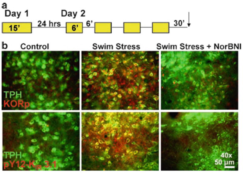
(a) Schematic of the repeated swim stress paradigm used for all studies. (b) Fluorescent images showing repeated swim stress increases both KORp-IR (red, top) and pY12-K_IR 3.1-IR (red, bottom) on TPH+ (green) and TPH- DRN neurons above basal activation found in “no stress” control animals and is sensitive to NorBNI (10 mg/kg) pretreatment.

Fig. 2. Stress-induced activation of KOR and p38 MAPK in same cells of the serotonergic dorsal-raphe nucleus.

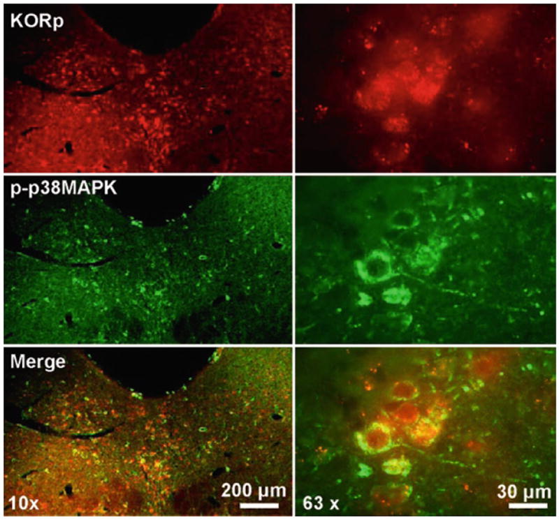
Fluorescent images of the dorsal-raphe nucleus following co-immunofluorescent staining with rabbit KORp and mouse phospho-p38 MAPK at 10× (right) and 63× (left) magnification. The image demonstrates that these proteins are activated following repeated stress and colocalized to the same cells.

3.5. Confocal and Epifluorescent Imaging

Epifluorescent microscopes are usually better for images taken at lower magnification (4–20×) that allow you to see gross neuro-anatomical structure, while confocal microscopes tend to better for higher magnifications (40–100×) and often work better with oil lenses (see Notes 10 and 11). Confocal microscopy is better when one is interested in subcellular localization of the protein of interest. Regardless of which microscope is being used, the general principles of image acquisition are the same.

3.5.1. Epifluorescent Microscopy

1. Most epifluorscent microscopes are equipped with CCD camera and accompanying software. Part of the software package contains a preview and look-up table component that can be used when acquiring the image. The look-up table contains measurements including exposure time, gain, and offset.

2. Take your set of slides and scan each slide by eye to quickly assess what section of what slide is the brightest/highest intensity of nonartifactual staining (if the perfusion was bad, some sections may have heavy blood vessel staining that will autofluoresce).

3. The look-up table will contain a histogram of the intensities for every pixel in the image. The exposure time, gain, and offset should be set such that the pixel intensity histogram is approximately Gaussian or slightly skewed to the left with few pixels oversaturated (see Note 12). It is important that the contrast is not adjusted so much so that the tissue texture is not discernable.

4. Once an exposure time, gain, and offset has been decided on for a given brain region, keep those settings consistent for all the subsequent image acquisition for all sections of all treatment groups for a given magnification. If you change to a different brain region or magnification, you must adjust the exposure time, gain, and offset appropriately. Sections with severe artifacts (see Note 13) should be excluded from quantification if using intensity measures (see Fig. 1).

3.5.2. Confocal Microscopy

1. Rather than a look-up table with exposure time, gain, and offset, confocal microscopes simply have dials to adjust gain and offset. A useful tool with the confocal software is the QLUT button that false colors the image based on the pixel intensity such that “black” pixels are labeled green, saturated pixels appear blue, and oversaturated pixels appear white. This is very helpful for making sure the image is balanced. A balanced image should have a moderately dense number of green pixels (about half the pixels) with some blue pixels and very few if any white pixels.

2. Once again an offset has been decided upon save that setting and use it for all the subsequent sections from all treatment groups (see Note 14).

3.6. Quantification

Analysis of phospho-selective immunoreactivity can be performed in two ways: intensity measurements and cell counts. Each method has specific drawbacks and therefore to obtain the clearest data, it is best to perform both these measurements for comparison (see Note 15).

3.6.1. Intensity Measurements

1. These instructions are based on the software MetaMorph Version 6.2r6 (Molecular Devices, Sunnyvale, CA), and assume use of the monoclonal antiphospho-p38 MAPK that detects dual phosphorylation of Thr180 and Tyr182, KORp, or pY12-K_IR 3.1. A minimum of three anatomically parallel tissue slices are necessary for a single data point.

2. Create and save a region that encompasses the area where you would expect to see a change in the phospho-antibody-IR. Create and save a second region of the same area where you would not expect to see a change in phospho-antibody-IR. Use these same regions on all analysis of tissue from the same experimental group.

3. Log the average pixel intensity in each of the regions. Repeat for all slices.

4. Calculate the ratio between the two regions, and average all anatomically parallel slices of a single individual (Fig. 3a) (see Note 16).

Fig. 3. Two different methods for quantifying immunohistochemistry data.

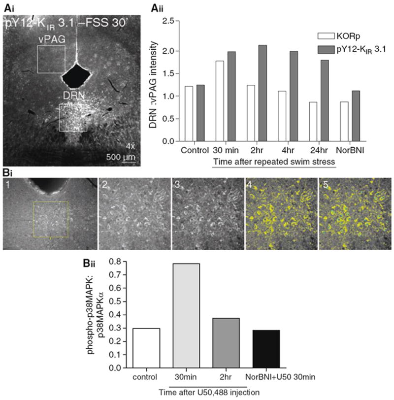
(Ai) An example image in which the intensities of two identically sized areas in the same section are compared from a stressor exposed animal. The serotonergic dorsal raphe demonstrates increases in pY12-K_IR3.1-IR while the ventral periaqueductal gray is unchanged. (Aii). A ratio is constructed the KORp or pY12-K_IR 3.1 DRN:vPAG intensity over a for three slices from a subject an averaged to generate a single N. The graph demonstrates a time course of KORp and pY12-K_IR 3.1 activation following repeated swim stress. Activation of both proteins is not present in subjects treated with the selective KOR antagonist norBNI. (Bi) Outlines the steps necessary when using the cell-counting technique to characterize the amount of phospho-immunoreactivity compared to the nonphospho-immunoreactivity. 1. Select region, 2. Zoom in on region, 3. “auto-enhance,” 4. set intensity threshold to one standard deviation above mean, 5. Toggle between threshold on/off and count cells that meet BOTH morphological AND intensity criterion. (Bii) An example experiment looking at the time course of p38 MAPK activation following intraperitoneal injection of the selective KOR agonist U50,488.

3.6.2. Cell Count

1. These instructions are based on the software MetaMorph Version 6.2r6 and can be used for any antibody that marks the activated form of a protein, costained with the antibody for the nonactivated form of the protein, both of which produce neuronal cell body staining. A minimum of three anatomically parallel tissue slices are necessary for a single data point.

2. Create and save a region that contains the area of interest. Use this same region on all analysis of tissue from the same experimental group.

3. Zoom in on the region and use “auto-enhance” to accentuate the contrast level of the image if need be. Set the inclusive threshold so that only pixels that have an intensity one standard deviation above the mean pixel intensity will be highlighted.

4. Count cells as active if they meet two criteria:

   1. Perimeter of the cell must be highlighted by the threshold (what percentage of the perimeter must be highlighted depends on the quality of staining, but must remain constant across an experimental group).
   2. Morphology of the cell must be appropriate and in focus (i.e., a visible nucleus).

5. Log the cell counts of each region and create a ratio of the number of cells with the activated form of the protein to the number of cells with the nonactivated form of the protein (Fig. 3b) (see Note 17).

References

- 1.Bruchas MR, Land BB, Aita M, Xu M, Barot SK, Li S, Chavkin C. Stress-induced p38 mitogen-activated protein kinase activation mediates kappa-opioid-dependent dysphoria. J Neurosci. 2007;27:11614–11623. doi: 10.1523/JNEUROSCI.3769-07.2007. [DOI] [PMC free article] [PubMed] [Google Scholar]
- 2.Bruchas MR, Xu M, Chavkin C. Repeated swim stress induces kappa opioid-mediated activation of extracellular signal-regulated kinase 1/2. Neuroreport. 2008;19:1417–1422. doi: 10.1097/WNR.0b013e32830dd655. [DOI] [PMC free article] [PubMed] [Google Scholar]
- 3.Thomas GM, Huganir RL. MAPK cascade signalling and synaptic plasticity. Nat Rev Neurosci. 2004;5:173–83. doi: 10.1038/nrn1346. [DOI] [PubMed] [Google Scholar]
- 4.Bardo MT, Bevins RA. Conditioned place preference: what does it add to our preclinical understanding of drug reward? Psychopharmacology (Berl) 2000;153:31–43. doi: 10.1007/s002130000569. [DOI] [PubMed] [Google Scholar]
- 5.Bolshakov VY, Carboni L, Cobb MH, Siegelbaum SA, Belardetti F. Dual MAP kinase pathways mediate opposing forms of long-term plasticity at CA3-CA1 synapses. Nat Neurosci. 2000;3:1107–1112. doi: 10.1038/80624. [DOI] [PubMed] [Google Scholar]
- 6.Bruchas MR, Macey TA, Lowe JD, Chavkin C. Kappa opioid receptor activation of p38 MAPK is GRK3- and arrestin-dependent in neurons and astrocytes. J Biol Chem. 2006;281:18081–18089. doi: 10.1074/jbc.M513640200. [DOI] [PMC free article] [PubMed] [Google Scholar]
- 7.Land BB, Bruchas MR, Schattauer S, Giardino WJ, Aita M, Messinger D, et al. Activation of the kappa opioid receptor in the dorsal raphe nucleus mediates the aversive effects of stress and reinstates drug seeking. Proc Natl Acad Sci U S A. 2009;106:19168–19173. doi: 10.1073/pnas.0910705106. [DOI] [PMC free article] [PubMed] [Google Scholar]
- 8.McLaughlin JP, Xu M, Mackie K, Chavkin C. Phosphorylation of a carboxyl-terminal serine within the kappa-opioid receptor produces desensitization and internalization. J Biol Chem. 2003;278:34631–34640. doi: 10.1074/jbc.M304022200. [DOI] [PubMed] [Google Scholar]
- 9.Ippolito DL, Xu M, Bruchas MR, Wickman K, Chavkin C. Tyrosine phosphorylation of K(ir)3.1 in spinal cord is induced by acute inflammation, chronic neuropathic pain, and behavioral stress. J Biol Chem. 2005;280:41683–41693. doi: 10.1074/jbc.M507069200. [DOI] [PMC free article] [PubMed] [Google Scholar]
- 10.Clayton CC, Bruchas MR, Lee ML, Chavkin C. Phosphorylation of the mu-opioid receptor at tyrosine 166 (Tyr3.51) in the DRY motif reduces agonist efficacy. Mol Pharmacol. 2010;77:339–347. doi: 10.1124/mol.109.060558. [DOI] [PMC free article] [PubMed] [Google Scholar]
- 11.Ippolito DL, Temkin PA, Rogalski SL, Chavkin C. N-terminal tyrosine residues within the potassium channel Kir3 modulate GTPase activity of Galphai. J Biol Chem. 2002;277:32692–32696. doi: 10.1074/jbc.M204407200. [DOI] [PMC free article] [PubMed] [Google Scholar]
- 12.Bausch SB, Patterson TA, Appleyard SM, Chavkin C. Immuno-cytochemical localization of delta opioid receptors in mouse brain. J Chem Neuroanat. 1995;8:175–189. doi: 10.1016/0891-0618(94)00044-t. [DOI] [PubMed] [Google Scholar]
- 13.Pan Z, Kao T, Horvath Z, Lemos J, Sul JY, Cranstoun SD, et al. A common ankyrin-G-based mechanism retains KCNQ and NaV channels at electrically active domains of the axon. J Neurosci. 2006;26:2599–25613. doi: 10.1523/JNEUROSCI.4314-05.2006. [DOI] [PMC free article] [PubMed] [Google Scholar]