Simplex Factor Models for Multivariate Unordered Categorical Data

Abstract

Gaussian latent factor models are routinely used for modeling of dependence in continuous, binary, and ordered categorical data. For unordered categorical variables, Gaussian latent factor models lead to challenging computation and complex modeling structures. As an alternative, we propose a novel class of simplex factor models. In the single-factor case, the model treats the different categorical outcomes as independent with unknown marginals. The model can characterize flexible dependence structures parsimoniously with few factors, and as factors are added, any multivariate categorical data distribution can be accurately approximated. Using a Bayesian approach for computation and inferences, a Markov chain Monte Carlo (MCMC) algorithm is proposed that scales well with increasing dimension, with the number of factors treated as unknown. We develop an efficient proposal for updating the base probability vector in hierarchical Dirichlet models. Theoretical properties are described, and we evaluate the approach through simulation examples. Applications are described for modeling dependence in nucleotide sequences and prediction from high-dimensional categorical features.

1. INTRODUCTION

Multivariate unordered categorical data are routinely encountered in a variety of application areas, with interest often in inferring dependencies among the variables. For example, the categorical variables may correspond to a sequence of A, C, G, T nucleotides or responses to questionnaire data on race, religion, and political affiliation for an individual. We shall use y_i = (y_i1, …, y_ip)^T to denote the multivariate observation for the ith subject, with y_ij ∈ {1, …, d_j}.

Complicated dependence can potentially be expressed in terms of simpler conditional independence relationships via graphical models (Dawid and Lauritzen 1993). Such models have been used for continuous (Lauritzen 1996; Dobra et al. 2004), categorical (Whittaker 1990; Madigan and York 1995), and mixed-scale variables (Pitt, Chan, and Kohn 2006; Dobra and Lenkoski 2011). Although graphical models are popular due to their flexibility and interpretability, computation is daunting since the size of the model space grows exponentially with p. Even with highly efficient search algorithms (Jones et al. 2005; Carvalho and Scott 2009; Dobra and Massam 2010; Lenkoski and Dobra 2011, among others), it is only feasible to visit a tiny subset of the model space even for moderate p. Accurate model selection in this context is difficult when p is moderate to large and the number of samples is not enormous because, in such cases, even the highest posterior probability models receive very small weight and there will typically be a large number of models having essentially identical performance according to any given model selection criteria (Akaike information criterion [AIC], Bayesian information criterion [BIC], etc). Dobra and Lenkoski (2011) advocated model averaging to avoid the inferences to depend explicitly on the choice of the underlying graph.

In parallel to the development of graphical models, factor models (West 2003; Carvalho et al. 2008) have been widely used for modeling of high-dimensional variables and dimension reduction. While Gaussian graphical models work with the precision matrix, factor models provide a framework for regularized covariance matrix estimation. Factor models and generalizations such as structural equation models (Bollen 1989) can accommodate mixtures of continuous, binary, and ordered categorical data through an underlying Gaussian latent factor structure (Muthén 1983). Such models link each observed y_ij to an underlying continuous variable z_ij, with ordinal y_ij arising via thresholding of z_ij. For multivariate binary y_i, a multivariate Gaussian distribution on z_i = (z_i1, …, z_ip)^T induces the multivariate probit model (Ashford and Sowden 1970; Chib and Greenberg 1998; Ochi and Prentice 1984). Multivariate probit models can accommodate nominal data with d_j > 2 by introducing a vector of variables z_ij = (z_ij1, …, z_ijdj)^T underlying y_ij, with y_ij = l if z_ijl = max z_ij (Aitchison and Bennett 1970; Zhang, Boscardin, and Belin 2008). The latent z_i’s are usually modeled as ${\sum }_{j=1}^p{d}_j$-dimensional Gaussian with covariance Σ, with at least p diagonal elements of Σ constrained to be one for identifiability. This constraint makes sampling from the full conditional posterior of Σ difficult. Zhang, Boscardin, and Belin (2006) used a parameter-expanded Metropolis–Hastings algorithm to obtain samples from a correlation matrix for multivariate probit models. Zhang, Boscardin, and Belin (2008) extended their algorithm to multivariate multinomial probit models. An alternative to probit models is to define a generalized linear model for each of the individual outcomes, while including shared normal latent traits to induce dependence (Sammel, Ryan, and Legler 1997; Dunson 2000, 2003; Moustaki and Knott 2000).

For unordered categorical variables, the data could be alternatively presented in the form of a p-way contingency table of dimension d₁ × ··· × d_p. There is a vast literature on analysis of contingency tables dating back to the nineteenth century. Fienberg and Rinaldo (2007) provided an excellent chronological overview of the development of log-linear models, maximum likelihood estimation, and asymptotic tests for goodness of fit. While log-linear models (Bishop, Fienberg, and Holland 1975) have been extensively used to model interactions among related categorical variables, asymptotic tests based on log-linear models face multiple difficulties in the case of sparse contingency tables—refer to the discussion in Section 3 of Fienberg and Rinaldo (2007). In a Bayesian framework, such problems can be avoided by specifying priors of the log-linear model parameters; Massam, Liu, and Dobra (2009) provided a detailed study of a useful class of conjugate priors. Posterior model search in log-linear models using traditional Markov chain Monte Carlo (MCMC) methods tends to bog down quickly as dimensionality increases. Dobra and Massam (2010) proposed a mode-oriented stochastic search method to more efficiently explore high posterior probability regions in decomposable, graphical, and hierarchical log-linear models.

Each of the above-mentioned methods are flexible and have their own distinct advantages. Graphical log-linear models are often preferred for ease of interpretation, while the underlying variable methods are useful for mixed data types, which commonly arise in social science applications. However, these methods face major computational challenges for large contingency tables. Dunson and Xing (2009) developed a nonparametric Bayes approach using Dirichlet process (Ferguson 1973, 1974) mixtures of product multinomials to directly model the joint distribution of multivariate unordered categorical data. They assumed that (y_i1, …, y_ip)^T are conditionally independent, given a univariate latent class index z_i ∈ {1, 2, …, ∞}. The prior specification is completed by assuming a stick-breaking process prior on the distribution of z_i and independent Dirichlet priors for the component-wise position-specific probability vectors. Marginalizing over the distribution of z_i induces dependence among the p variables. This approach extends latent structure analysis (Lazarsfeld and Henry 1968; Goodman 1974) to the infinite mixture case and is conceptually related to nonnegative tensor decompositions (Shashua and Hazan 2005; Kimand Choi 2007). The direct modeling of the joint distribution of the category probabilities in a sparse manner enables efficient posterior computation, thereby allowing their method to efficiently scale up to high dimensions.

Although the Dunson and Xing (2009) approach can handle large contingency tables, the assumption of conditional independence, given a single latent class index, seems restrictive. Although their prior has full support and hence they can flexibly approximate any joint distribution of y_i, in practice, even relatively simple dependence structures may require allocation of individuals to different classes, leading to a large effective number of parameters. Hence, in applications involving moderate to large p and modest sample size n, the Dunson and Xing (2009) approach may face difficulties.

In this article, we propose a new class of simplex factor models for multivariate unordered categorical data in which the dependence among the high-dimensional variables is explained in terms of relatively few latent factors. This is akin to Gaussian factor models, but factors on the simplex are more natural for nominal data. Methods for factor selection are discussed and the proposed approach is shown to have large support and to lead to consistent estimation of joint or conditional distributions for categorical variables. The Dunson and Xing (2009) model is obtained as a particular limiting case of the proposed model, as is the product multinomial model. The joint distribution of the multivariate nominal variables induced from the simplex factor model is shown to correspond to a multilinear singular value decomposition (SVD) (or higher-order SVD [HOSVD]) (De Lathauwer, De Moor and Vandewalle 2000) of probability tensors, which is regarded as a natural generalization of the matrix SVD in the tensor literature. A simple-to-implement data-augmented MCMC algorithm is proposed for posterior computation that scales well to higher dimensions. The methods are illustrated through simulated and real-data examples.

2. MODEL AND PRIOR SPECIFICATION

2.1 The Simplex Factor Model

Let y_i = (y_i1, …, y_ip)^T denote a vector of responses and/or predictors. If y_i ∈ ℜ^p, then a common approach is to jointly model the y_i’s via a normal linear factor model:

$$y_i=\mu +\mathrm{\Lambda }{\eta }_i+{\epsilon }_i,{\epsilon }_i~N_p(0,\mathrm{\sum }),i=1,\dots ,n,$$ (1)

where μ ∈ ℜ^p is an intercept term, Λ is a p × k factor loadings matrix, η_i ∈ ℜ^k are latent factors, and ε_i is an idiosyncratic error with covariance $\mathrm{\sum }=\text{diag}({\sigma }_1^2,\dots ,{\sigma }_p^2)$. When η_i ~ N_k(0, I_k), marginally, y_i ~ N_p(μ, Ω), with Ω = ΛΛ^T + Σ, a decomposition which uses at most p(k + 1) free parameters instead of the p(p + 1)/2 parameters in an unstructured covariance matrix.

Now consider the case in which y_ij ∈ {1, …, d_j} for j = 1, …, p, and the different observations are unordered categorical variables. Let η_i = (η_i1, …, η_ik)^T ∈ , with the (k − 1)-dimensional simplex. The η_i’s will play the role of the latent factors but they lie on the simplex instead of being in ℜ^k. In addition, for each j, let ${\mathbf{\lambda }}_h^{(j)}={({\lambda }_{h1}^{(j)},\dots ,{\lambda }_{{hd}_j}^{(j)})}^{\text{T}}$ be a probability vector for h = 1, …, k. The ${\mathbf{\lambda }}_h^{(j)}$’s can be interpreted as loadings for factor h and outcome j, but we have a vector instead of a single element, as we would have in the case in which y_ij ∈ ℜ. With these components, we let:

$$\text{pr}(y_{ij}=c_j\mid {\eta }_i,\mathbf{\Lambda })=\sum _{h=1}^k{\lambda }_{{hc}_j}^{(j)}{\eta }_{ih}$$ (2)

$$\text{pr}(y_{i1}=c_1,\dots ,y_{ip}=c_p\mid {\eta }_i,\mathbf{\Lambda })=\prod _{j=1}^p\text{pr}(y_{ij}=c_j\mid {\eta }_i,\mathbf{\Lambda }),$$ (3)

where $\mathbf{\Lambda }=({\mathbf{\lambda }}_h^{(j)})$. We refer to the model defined in Equations (2) and (3) as a simplex factor model. The formulation is conceptually related to mixed membership models (Pritchard, Stephens, and Donnelly 2000; Barnard et al. 2003; Blei, Ng, and Jordan 2003; Erosheva, Fienberg, and Joutard 2007), which have found widespread applications in text modeling, population genetics, and machine learning. In particular, the latent Dirichlet allocation (LDA) model (Blei et al. 2003) for text modeling arises as a special case of our model when p = 1. We can think of ${\mathbf{\lambda }}_h^{(j)}$ as the vector of probabilities of y_ij = 1, 2, …, d_j, respectively, in ancestral population or pure species h, with none of the individuals being pure and η_ih being the weight on the hth component for the ith individual. When k = 1, the simplex factor model reduces to the product multinomial model representing global independence. As k increases, the complexity of the model increases.

To obtain further insight, we represent the simplex factor model in the following hierarchical form, which will also be used for posterior computation:

$$y_{ij}~\text{multinomial}(\{1,\dots ,d_j\},{\lambda }_{z_{ij}1}^{(j)},\dots ,{\lambda }_{z_{ij}{d}_j}^{(j)}),\text{pr}(z_{ij}=h)={\eta }_{ih},h=1,\dots ,k.$$ (4)

Clearly, marginalizing out z_ij in (4) gives (2). The z_ij’s can be considered as local latent class indices for the jth variable and the ith subject. The simplex factor model allows these local indices z_ij’s to vary across j for a particular subject, resulting in a more flexible and parsimonious (in terms of number of components k) specification compared with that in Dunson and Xing (2009), where a univariate latent class index is used.

Marginalizing out η_i in Equation (3) induces dependence among the y_ij’s. Letting π_c1…c^p = pr(y_i1 = c₁, …, y_ip = c_p | Λ), one has

$$\begin{array}{l}{\pi }_{c_1\dots c_p}=\int \prod _{j=1}^p\text{pr}(y_{ij}=c_j\mid {\eta }_i,\mathbf{\Lambda })d\mathcal{Q}({\eta }_i)\\ =\sum _{h_1=1}^k\dots \sum _{h_p=1}^k{g}_{h_1\dots h_p}\prod _{j=1}^p{\lambda }_{h_j{c}_j}^{(j)},\end{array}$$ (5)

with denoting the distribution of η_i and g_h1,…,hp = E(η_ih1, …, η_ihp).

2.2 Relationship With Tensor Decompositions

It is useful at this point to consider relationships between (5) and the literature on tensor decompositions, which shall be used in particular to illustrate the differences between our model and the Dunson and Xing (2009) model. Let denote the set of all tensors of dimension d₁ × ··· × d_p, and Π_d1…dp ⊂ denote the set of probability tensors so that π ∈ Π_d1…dp implies

$$\mathit{\pi }=\{{\pi }_{c_1\dots c_p}\ge 0,c_j=1,\dots ,d_j,j=1,\dots ,p:\sum _{c_1=1}^{d_1}\dots \sum _{c_p=1}^{d_p}{\pi }_{c_1\dots c_p}=1\}.$$

A decomposed tensor (Kolda 2001) is a tensor D ∈ such that D = u⁽¹⁾ ⊗ u⁽²⁾, …, ⊗u^(p), where u^(j) ∈ ℜ^d_j and ⊗ denotes the outer product so that $D_{c_1,\dots ,c_p}=u_{c_1}^{(1)}{u}_{c_2}^{(2)},\dots ,u_{c_p}^{(p)}$. One notion of the rank of a tensor is the minimal r such that D can be expressed as a sum of r decomposed (or rank 1) tensors. Such a decomposition is often referred to as a PARAFAC decomposition (Harshman 1970), which is one way of generalizing the matrix SVD. Tucker (1966) proposed a different decomposition for three-way data, which was later extended to arbitrary tensors by De Lathauwer et al. (2000). The Tucker decomposition or HOSVD aims to decompose a tensor D ∈ as

$$D_{c_1\dots c_p}=\sum _{h_1=1}^{d_1}\dots \sum _{h_p=1}^{d_p}{g}_{h_1,\dots ,h_p}{u}_{h_1{c}_1}^{(1)},\dots ,u_{h_p{c}_p}^{(p)},$$ (6)

where G = {g_h1…hp} ∈ is called a core tensor and its entries control interaction between the different components. Wang and Ahuja (2005) and Kim and Choi (2007) empirically noted that the HOSVD achieves better data compression and requires fewer components compared with the PARAFAC model as it uses all combinations of the mode vectors $u_h^{(j)}$’s, h = 1, …, k.

The product multinomial mixture model of Dunson and Xing (2009) induces a decomposition of a probability tensor π as

$${\pi }_{c_1\dots c_p}=\sum _{h=1}^k{\nu }_h{\lambda }_{{hc}_1}^{(1)},\dots ,{\lambda }_{{hc}_p}^{(p)},$$ (7)

where ν_h = pr(z_i = h) and ${\mathbf{\lambda }}_h^{(j)}\in {\mathcal{S}}_{d_j-1}$. Note that (7) is different from a usual PARAFAC decomposition because of the nonnegativity constraints on ν and the ${\mathbf{\lambda }}_h^{(j)}$’s. In the subsequent discussion, a nonnegativity matrix/tensor has all entries nonnegativity. The classical nonnegativity matrix factorization (NMF) problem seeks the best approximation of a nonnegative matrix $A\in {\mathfrak{R}}_{+}^{m\times n}$ as a product of nonnegative matrices $W\in {\mathfrak{R}}_{+}^{m\times k}$ and $V\in {\mathfrak{R}}_{+}^{k\times n}$ for some k ≤ min{m, n}. Gregory and Pullman (1983) were among the first to consider NMF and introduced the notion of nonnegative rank of a matrix, which is the minimal r such that a nonnegative matrix can be written as a sum of rank 1 nonnegative matrices. Cohen and Joel (1993) generalized many properties of the usual rank to the case of nonnegative rank. Along the lines of NMF, one can similarly envision nonnegative versions of the PARAFAC and HOSVD decompositions for tensors (Shashua and Hazan 2005; Kimand Choi 2007).

We note that (7) is a form of nonnegative PARAFAC decomposition, while the simplex factor model in (5) induces a nonnegative HOSVD on the space of probability tensors. Let $\mathit{\pi }\in {\mathcal{T}}_{d_1\dots d_p}^{+}$ be a nonnegative tensor. Define the nonnegative PARAFAC rank ${\text{r}}_{\text{PF}}^{+}(\mathit{\pi })$ of π to be the minimum k such that π admits a decomposition as in (7)with ${\mathbf{\lambda }}_h^{(j)}\in {\mathcal{S}}_{d_j-1}$ and ν ∈ ℜ^k. Similarly, define the nonnegative HOSVD rank ${\text{r}}_{\text{HS}}^{+}(\mathit{\pi })$ of π to be the minimum k such that π can be expressed as in (5) with ${\mathbf{\lambda }}_h^{(j)}\in {\mathcal{S}}_{d_j-1}$ and $\mathbf{G}\in {\mathcal{T}}_{k\dots k}^{+}$. In considering a nonnegative decomposition, assuming ${\mathbf{\lambda }}_h^{(j)}\in {\mathcal{S}}_{d_j-1}$ is not restrictive since we can always scale nonnegative weights to lie to the simplex and adjust the scale in ν or G. In the special case when π is a probability tensor, ν ∈ is a probability vector and G is a probability tensor.

If we start with $k={\text{r}}_{\text{PF}}^{+}(\mathit{\pi })$ in (7), then we can clearly express π as in (5) using the same k by simply letting g_h1…hp = ν_h1(h₁ = h, …, h_p = h). Conversely, suppose we start with a nonnegative HOSVD of π as in (5) with $k={\text{r}}_{\text{HS}}^{+}(\mathit{\pi })$ and the core tensor G ∈ Π_k…k having ${\text{r}}_{\text{PF}}^{+}(\mathbf{G})=r$. Then, there exist ${\mathbf{u}}_l^{(j)}\in {\mathcal{S}}_{k-1}$, l = 1, …, r and q ∈ such that $g_{h_1\dots h_p}={\sum }_{l=1}^r{q}_l{u}_{{lh}_1}^{(1)},\dots ,u_{{lh}_p}^{(p)}$. Substituting this expression for g_h1…hp in (5), one has

$$\begin{array}{l}{\pi }_{c_1\dots c_p}=\sum _{h_1=1}^k\dots \sum _{h_p=1}^k{g}_{h_1\dots h_p}{\lambda }_{h_1{c}_1}^{(1)},\dots ,{\lambda }_{h_p{c}_p}^{(p)}\\ =\sum _{l=1}^r{q}_l\left\{\prod _{j=1}^p\left(\sum _{h=1}^k{\lambda }_{{hc}_j}^{(j)}{u}_{lh}^{(j)}\right)\right\}=\sum _{l=1}^r{q}_l{v}_{l{c}_1}^{(1)},\dots ,v_{l{c}_p}^{(p)},\end{array}$$ (8)

where $v_{l{c}_j}^{(j)}={\sum }_{h=1}^k{\lambda }_{{hc}_j}^{(j)}{u}_{lh}^{(j)}$. Thus, starting with a nonnegative HOSVD of π, we have expanded it in nonnegative PARAFAC form. Clearly, r ≥ k; otherwise, the minimality of k is contradicted. Moreover, very little is known about upper bounds on PARAFAC ranks of tensors. The most general result is for third-order tensors where the upper bound is O(k²); hence, r can potentially be much larger than k, requiring very many parameters for the PARAFAC expansion compared with the HOSVD. We summarize the above facts in the following theorem.

Theorem 2.1

Let π ∈ Π_d1…dp and let $k={\text{r}}_{\text{HS}}^{+}(\mathit{\pi })$. Then, $k\le {\text{r}}_{\text{PF}}^{+}(\mathit{\pi })\le {\text{r}}_{\text{PF}}^{+}(\mathbf{G})$, where G is a core tensor in the minimal HOSVD expansion of π. Moreover, among all such minimal expansions in k components, if G has minimal nonnegative PARAFAC rank, then ${\text{r}}_{\text{PF}}^{+}(\mathit{\pi })={\text{r}}_{\text{PF}}^{+}(\mathbf{G})$.

From a statistical perspective, the decomposition in (8) shows that the simplex factor model can provide sparser solutions in scenarios where the Dunson and Xing (2009) model may require many components to adequately explain the dependence structure. The Dunson and Xing (2009) model induces a global clustering phenomenon by forcing all the variables for a particular subject to be allocated to the same cluster. This can lead to introduction of too many clusters to accommodate small idiosyncracies within the variables or the subjects might be inappropriately grouped together, obscuring local differences. The simplex factor model instead allows the different variables to be allocated to different clusters via the dependent local cluster indices z_ij.

2.3 Prior Specification and Properties

To complete a Bayesian specification of the simplex factor model, a natural choice is to draw the η_i’s and the different ${\mathbf{\lambda }}_h^{(j)}$’s from independent Dirichlet priors. We let η_i ~ Diri(αν₁, …, αν_k), where α > 0 and ν = (ν₁, …, ν_k)^T = E(η_i) ∈ is a vector of probabilities. To obtain a parsimonious representation in which the first few components (subpopulations) tend to be assigned most of the weight, we let ${\nu }_h={\nu }_h^{\ast }{\mathrm{\Pi }}_{l<h}(1-{\nu }_l^{\ast })$ with ${\nu }_k^{\ast }=1$ and place a beta(1, β) prior on ${\nu }_h^{\ast }$, h = 1, …, k − 1. This corresponds to the stick-breaking formulation (Sethuraman 1994) of the Dirichlet process truncated to the first k terms and is widely used for posterior computation in Dirichlet process mixture models (Ishwaran and James 2001). In this case, k can be viewed as an upper bound on the number of components as higher-indexed components will tend to have ν_h ≈ 0, so one obtains η_ih ≈ 0 with high probability for all i and the k-component model adaptively collapses on a lower-dimensional model. In practice, such collapsing will be driven by the extent to which the data support a model with fewer components. The model can be expressed in hierarchical form as

$$\begin{array}{l}{y}_{ij}~\text{multinomial}(\{1,\dots ,d_j\},{\lambda }_{z_{ij}1}^{(j)},\dots ,{\lambda }_{z_{ij}{d}_j}^{(j)}),\\ {\mathbf{\lambda }}_h^{(j)}~\text{Diri}(a_{j1},\dots ,a_{{jd}_j}),\text{pr}(z_{ij}=h)={\eta }_{ih},\\ {\eta }_i~\text{Diri}(\alpha \mathit{\nu }),{\nu }_h={\nu }_h^{\ast }\prod _{l<h}(1-{\nu }_l^{\ast }),{\nu }_h^{\ast }~\text{beta}(1,\beta ).\end{array}$$ (9)

The hierarchical prior specification on η_i has similarities to a finite-dimensional version of the hierarchical Dirichlet process (Teh et al. 2006), although the motivation here is slightly different. Essentially, we have a Dirichlet random-effects model with an unknown mean for the subject-specific random effects η_i’s, with dependence being induced by marginalizing out the η_i’s.

The Dirichlet latent factor distribution allows evaluation of g_h1…hp = E(η_{ih1 … ηihp}) in (5) analytically

$$g_{h_1\dots h_p}=\frac{\mathrm{\Gamma }(\alpha )}{\mathrm{\Gamma }(\alpha +p)}\prod _{h=1}^k\frac{\mathrm{\Gamma }\{\alpha {\nu }_h+{\tau }_h(h_1,\dots ,h_p)\}}{\mathrm{\Gamma }(\alpha {\nu }_h)},$$ (10)

where τ_h(h₁, …, h_p) = {#j: h_j = h} for h = 1, …, k. When evident from the context, we shall drop the arguments and use τ_h. Clearly, ${\sum }_{h=1}^k{\tau }_h=p$.

With ${\pi }_{c_j}^{(j)}=\text{pr}(y_{ij}=c_j\mid \mathit{\nu },\mathbf{\Lambda })$ and ${\pi }_{c_j{c}_{j^{\prime }}}^{(j{j}^{\prime })}=\text{pr}(y_{ij}=c_j,y_{i{j}^{\prime }}=c_{j^{\prime }}\mid \mathit{\nu },\mathbf{\Lambda })$, one has

$${\pi }_{c_j}^{(j)}=\sum _{h=1}^k{\nu }_h{\lambda }_{{hc}_j}^{(j)}$$ (11)

$${\pi }_{c_j{c}_{j^{\prime }}}^{(j{j}^{\prime })}=\frac{\alpha }{\alpha +1}\left(\sum _{h=1}^k{\nu }_h{\lambda }_{{hc}_j}^{(j)}\right)\left(\sum _{h=1}^k{\nu }_h{\lambda }_{{hc}_{j^{\prime }}}^{(j^{\prime })}\right)+\frac{1}{\alpha +1}\sum _{h=1}^k{\nu }_h{\lambda }_{{hc}_j}^{(j)}{\lambda }_{{hc}_{j^{\prime }}}^{(j^{\prime })}.$$ (12)

Now let us consider a few limiting cases; the main results are summarized below.

Proposition 2.2

For any fixed k, (i) in the limit as α → ∞, the simplex factor model (9) simplifies to a product multinomial model with $\text{pr}(y_{ij}=c_j)={\sum }_{h=1}^k{\nu }_h{\lambda }_{{hc}_j}^{(j)}$ independently for j = 1, …, p; and (ii) in the limit as α → 0, model (9) simplifies to the Dunson and Xing (2009) model.

Thus, by putting a hyperprior on α, we can allow the data to inform about α and the posterior to concentrate near either of these two simplifications in cases where the simple structure is warranted. Next, we show that the proposed prior has large support on the space of probability tensors, so any dependence structure can be accurately approximated.

Theorem 2.3

Let ${\mathcal{Q}}_{\pi }^{(k)}$ denote the prior induced on Π_d1…dp through the k-component simplex factor model in (9) and (π⁰) denote an L₁ neighborhood around an arbitrary probability tensor π⁰ ∈ Π_d1…dp. Then, for any π₀ ∈ Π_d1…dp and ε > 0, there exists k such that ${\mathcal{Q}}_{\pi }^{(k)}\{{\mathcal{N}}_{\epsilon }({\mathit{\pi }}^0)\}>0$.

Since the space of probability tensors is isomorphic to a compact Euclidean space, a straightforward extension of theorem 4.3.1 of Ghosh and Ramamoorthi (2003) ensures that the posterior concentrates in arbitrary small neighborhoods of any true data-generating distribution π⁰ with increasing sample size.

3. POSTERIOR COMPUTATION AND INFERENCE

3.1 MCMC Algorithm for Posterior Computation

Let y = (y_ij), η = (η_i), and z = (z_i). We use a combination of Gibbs sampling and independence chain Metropolis–Hastings sampling to draw samples from the posterior distribution of (Λ, z, η, ν^*,α) for the hierarchical model specified in (9). We place a gamma(a_α, b_α) prior on α to allow the data to inform more strongly about sparsity in the η_i vectors. In particular, for small α, the tendency will be to assign one element of η_i to a value close to 1, while for larger α, the η_i vectors will be closer to ν for different subjects. We recommend a_α = b_α = 1 as a default value favoring high weights on few components. In addition, we let a_j1 = ··· = a_jdj= 1, for j = 1, …, p, to induce a uniform prior for the category probabilities in each class for each outcome type. This default prior specification can be modified in cases in which one has prior information on the category probabilities and/or the number of subpopulations.

The conditional posteriors for all the parameters other than ν^* and α can be derived in closed form using standard algebra and the sampler cycles through the following steps:

• Step 1
  For h = 1, …, k, update ${\mathbf{\lambda }}_h^{(j)}$ from the following Dirichlet full conditional posterior distribution

  $$\pi ({\mathbf{\lambda }}_h^{(j)}\mid -)~\text{Diri}\left(a_{j1}+\sum _{i:z_{ij}=h}1(y_{ij}=1),\dots ,a_{{jd}_j}+\sum _{i:z_{ij}=h}1(y_{ij}=d_j)\right)$$
• Step 2
  Update z_ij from the multinomial full conditional posterior distribution, with

  $$\text{pr}(z_{ij}=h\mid -)=\frac{{\eta }_{ih}{\lambda }_{{hy}_{ij}}^{(j)}}{{\sum }_{l=1}^k{\eta }_{il}{\lambda }_{{ly}_{ij}}^{(j)}}.$$
• Step 3
  Update η_i from the Dirichlet full conditional posterior:

  $$\pi ({\eta }_i\mid -)~\text{Diri}\left(\alpha {\nu }_1+\sum _{j=1}^{p}1(z_{ij}=1),\dots ,\alpha {\nu }_k+\sum _{j=1}^{p}1(z_{ij}=k)\right).$$
• Step 4Update α using a Metropolis random walk on log(α).
• Step 5
  Update { ${\nu }_h^{\ast }$} using the following approach. Let $m_{il}={\sum }_{j=1}^{p}1(z_{ij}=l),m_l={\sum }_{i=1}^n{m}_{il},m_{l+}={\sum }_{i=1}^n{\sum }_{l^{\prime }>1}{m}_{i{l}^{\prime }}$ and n_ls = {#i: m_il > s} for nonnegative integers s. Letting $m_l^{\ast }={max}_{1\le i\le n}{m}_{il}$, one has n_ls = 0 for $s\ge m_l^{\ast }$. Further, let ${\stackrel{\sim }{\nu }}_h^{(h)}={\mathrm{\Pi }}_{l<h}(1-{\nu }_l^{\ast })$ and ${\stackrel{\sim }{\nu }}_l^{(h)}={\nu }_l/(1-{\nu }_h^{\ast })$ for l > h, and define $c_l^{(h)}=\alpha {\stackrel{\sim }{\nu }}_l^{(h)}$. The conditional posterior of ${\nu }_h^{\ast }$ marginalizing out the η_i’s is given by

  $$\begin{array}{l}\pi ({\nu }_h^{\ast }\mid -)\propto {(1-{\nu }_h^{\ast })}^{\beta -1}\prod _{i=1}^n\prod _{l=h}^k\frac{\mathrm{\Gamma }(\alpha {\nu }_l+m_{il})}{\mathrm{\Gamma }(\alpha {\nu }_l)}\\ ={(1-{\nu }_h^{\ast })}^{\beta -1}\prod _{l=h}^k\prod _{i:m_{il}\ne 0}\prod _{s=0}^{m_{il}-1}(\alpha {\nu }_l+s).\end{array}$$ (13)

  We assume the default choice β = 1. Since the expression for ν_l contains ${\nu }_h^{\ast }$ for l = h and ( $1-{\nu }_h^{\ast }$) for l > h, the conditional posterior of ${\nu }_h^{\ast }$ in (13) is an analytically intractable mixture of beta densities. However, we show that $\pi ({\nu }_h^{\ast }\mid -)$ can be accurately approximated by a single beta distribution. One can thus use an appropriate beta density as a proposal in a Metropolis–Hastings step, with the beta parameters estimated numerically on a fine grid via moment matching. However, the grid-based method is computationally costly, since the expression in (13) needs to be computed at every point on the grid. We propose an approach to provide analytic expressions for the parameters of the approximating beta density. The analytic solution produces high acceptance rates, and there is a dramatic gain in computational time, whose effect is increasingly pronounced with large n and/or p. We mention below the choices of the parameters of the approximating beta density in the different cases, with justification provided in the Appendix.

If m_h > 0 and m_h+ = 0, we use a beta(â, 1) density with

$$\widehat{a}=1+\sum _{s=0}^{m_h^{\ast }-1}{n}_{hs}\left\{1-\frac{s}{c_h^{(h)}}log(1+c_h^{(h)}/s)\right\}$$ (14)

to approximate $\pi ({\nu }_h^{\ast }\mid -)$. Similarly, if m_h = 0 and m_h+ > 0, a beta(1, b̂) density with

$$\widehat{b}=1+\sum _{l=h+1}^k\sum _{s=0}^{m_l^{\ast }-1}{n}_{ls}\left\{1-\frac{s}{c_l^{(h)}}log(1+c_l^{(h)}/s)\right\}$$ (15)

is used to approximate $\pi ({\nu }_h^{\ast }\mid -)$.

If m_h > 0 and m_h+ > 0, we prove the following fact.

Proposition 3.1

If m_h > 0 and m_h+ > 0, then $\pi ({\nu }_h^{\ast }\mid -)$ is unimodal and ${lim}_{{\nu }_h^{\ast }\to 0}\pi ({\nu }_h^{\ast }\mid -)=0,{lim}_{{\nu }_h^{\ast }\to 1}\pi ({\nu }_h^{\ast }\mid -)=0$.

We approximate $\pi ({\nu }_h^{\ast }\mid -)$ by a beta(â, b̂) density in this case, where â = max(ã + 1, 1), b̂ = max(b̃ + 1, 1), and ã, b̃ are obtained by solving a 2 × 2 linear system E(ã, b̃)^T = (d₁, d₂)^T, with e₁₁ = 1/2, e₁₂ = −1/2, e₂₁ = 1/6, e₂₂ = −1/3 and

$$\begin{array}{l}{d}_1={\int }_0^{1}2{\nu }_h^{\ast }log\pi ({\nu }_h^{\ast }\mid -)d{\nu }_h^{\ast }-{\int }_0^{1}log\pi ({\nu }_h^{\ast }\mid -)d{\nu }_h^{\ast }\\ d_2={\int }_0^{1}3{({\nu }_h^{\ast })}^{2}log\pi ({\nu }_h^{\ast }\mid -)d{\nu }_h^{\ast }-{\int }_0^{1}2{\nu }_h^{\ast }log\pi ({\nu }_h^{\ast }\mid -)d{\nu }_h^{\ast }.\end{array}$$

A one-step improvement is obtained next by running a mode search of the log posterior from the estimated (ã, b̃) pair above and subsequently adjusting those values to have the right mode. Since $\pi ({\nu }_h^{\ast }\mid -)$ is unimodal in this case, the mode search can be done very efficiently using the Newton–Rapson algorithm.

3.2 Adaptive Selection of the Number of Factors

In practical problems, one typically expects a small number of factors k relative to the number of outcomes p. The stick-breaking prior on ν induces a sparse formulation a priori, so relatively few components with high weights are encouraged. Accordingly, one can start with a conservative upper bound k^* on the number of factors and the sparsity favoring prior ensures that the posterior will concentrate on a few components if the truth is approximately sparse. However, an overly conservative upper bound wastes substantial computational time. For Gaussian factor models, Lopes and West (2004) compared a number of alternatives to select the number of factors, recommending a reversible-jump MCMC approach that requires a preliminary run for each choice of the number of factors, which is very computationally intensive. Since we are not interested in inference on the number of factors and our sole consideration is computational efficiency, we outline below a simple adaptive scheme to discard the redundant factors in a tuning phase and continue with a smaller number of factors for the remainder of the chain. This results in considerable computational gains in high dimensions; however, for moderate values of p (e.g., p ≤ 20), one can set p to be the truncation level and ignore the adaptive scheme.

We reserve T_tune many iterations at the beginning of the chain for tuning. At iteration t, letting $K_{\text{eff}}^{(t)}\subset \{1,\dots ,k\}$ to denote the unique values among the z_ij’s, one clearly has m_h > 0 if and only if $h\in K_{\text{eff}}^{(t)}$. We define the effective number of factors k̃^(t) as | $K_{\text{eff}}^{(t)}$|. The inherent sparse structure of the simplex factor model favors small values of k̃^(t). Starting with a conservative guess for k, we monitor the value of k̃^(t) every 50 iterations in the tuning phase. If there are no redundant factors, that is, m_h > 0 for all h, we add a factor and initialize the additional parameters for η, Λ, ν^* from the prior. Otherwise, we delete the redundant components and retain the elements of η, Λ, ν^* corresponding to $h\in K_{\text{eff}}^{(t)}$. In either case, we normalize the samples for η and ν^* to ensure they lie on the simplex. We continue the chain with the updated number of factors and the modified set of parameters for the next 50 iterations before making the next adaptation. At the end of the tuning phase, we fix the number of factors for the remainder of the chain at the value corresponding to the last adaptation. In all our examples, we let T_tune = 5000 and choose the initial number of factors as 20 or 10.

3.3 Inference

One can estimate the marginal distribution of the y_ij’s and conduct inferences on the dependence structure based on the MCMC output and using the expressions for the lower-dimensional marginals in Equations (11) and (12). To conduct inference on dependence between y_ij and y_ij′ for j ≠ j′ ∈ {1, …, p}, we consider the pairwise normalized mutual information matrix M = (m_jj′), with m_jj′ = I_jj′/{H_jH_j′}^0.5 and

$$\begin{array}{l}{I}_{j{j}^{\prime }}=\sum _{c_j=1}^{d_j}\sum _{c_{j^{\prime }}=1}^{d_{j^{\prime }}}{\pi }_{c_j{c}_{j^{\prime }}}^{(j{j}^{\prime })}log\left\{\frac{{\pi }_{c_j{c}_{j^{\prime }}}^{(j{j}^{\prime })}}{{\pi }_{c_j}^{(j)}{\pi }_{c_{j^{\prime }}}^{(j^{\prime })}}\right\},\\ H_j=-\sum _{c_j=1}^{d_j}{\pi }_{c_j}^{(j)}log\{{\pi }_{c_j}^{(j)}\}.\end{array}$$

The mutual information I_jj′ is a general measure of dependence between a pair of random variables (Y_J, Y_j′), with I_jj′ = 0 if and only if Y_j and Y_j′ are independent. Using our Bayesian approach, one can obtain samples from the posterior distribution of m_jj′ for all j ≠ j′ pairs. In particular, posterior summaries of the p × p association matrix can be used to infer on the association between pairs of variables accounting for uncertainty in other variables. Dunson and Xing (2009) pointed out that in large model spaces, it is more computationally tractable to consider pairwise marginal dependencies as compared with learning the entire graph of conditional dependencies. Dunson and Xing (2009) and Dobra and Lenkoski (2011) used the pairwise Cramer’s V association matrix as a measure of dependence. We also computed the pairwise Cramer’s V association matrix for all our examples and obtained similar dependence structures as found by the mutual information criterion. In the analysis of the Rochdale data in Section 4, we present results for both measures of association and in the subsequent simulated and real-data examples, we only provide the results for the mutual information criterion as the conclusions were similar.

In many practical examples, one routinely encounters a high-dimensional vector of nominal predictors y_i along with nominal response variables u_i, with interest in building predictive models for u_i given y_i. For example, y_i might correspond to a nucleotide sequence, with u_i being the existence/nonexistence of some special feature within the gene sequence. By using a simplex factor model for the joint distribution of the response and predictors, one obtains a very flexible approach for classification from categorical predictors that may have higher-order interactions. Such a joint model also trivially allows imputation of missing values under the missing at-random assumption or any other informative missingness.

4. ANALYSIS OF ROCHDALE DATA

Dobra and Lenkoski (2011) used copulas to extend traditional Gaussian graphical models to allow mixed outcomes. They applied their general class of copula Gaussian graphical models (CGGM) to analyze the Rochdale data, a 2⁸ contingency table popular in the social science literature. In this section, we illustrate various aspects of making inference with the simplex factor model on this well-known dataset and compare our results with the CGGM.

The Rochdale dataset was previously analyzed in Whittaker (1990). It is a social survey dataset aimed to assess the relationship among factors influencing women’s economic activity. The dataset consists of eight related binary variables coded a, b, …, h for n = 665 women. A detailed account of the different variables can be found in Dobra and Lenkoski (2011). The resulting 2⁸ contingency table is sparse, with 165 cell counts of zero. The top 10 cell counts are all greater than 20.

Whittaker (1990) used log-linear models to analyze this dataset and argued against using higher-order interactions involving more than two variables. He considered two log-linear models, one being the all two-way interaction model, and the minimal sufficient statistics for the other one consisted of 14 two-way marginals in equation 5.1 of Dobra and Lenkoski (2011). Dobra and Lenkoski (2011) analyzed this dataset using their proposed CGGM and also compared it with a copula full model where the underlying graph was not updated and was fixed at the full graph.

The simplex factor model was run for 50,000 iterations, with the first 30,000 iterations discarded as burn-in and every fifth sample post burn-in was collected. We started with 10 factors and the adaptive algorithm selected four factors, with more than 85% acceptance rate for all elements of ν^*. The posteriormean of α was 0.10, with a 95% credible interval of (0.03–0.20).

According to Whittaker (1990), the strongest pairwise interaction in this dataset is for the pair (b, d), followed by (b, h), (e, f), and (a, g). Dobra and Lenkoski (2011) obtained strongest associations for the pairs (b, d), (b, h), (a, g), (e, f), and (c, g) according to Cramer’s V statistic. They also noted that conditioning on the full graph in the copula full model leads to severe underestimation of all the pairwise Cramer’s V associations. From the MCMC output, we obtained posterior samples for the pairwise normalized mutual information and the pairwise Cramer’s V. Figure 1 shows posterior summaries of the pairwise associations for these two measures. From Figure 1, it is evident that both measures obtained a similar dependence structure and the top four pairs according to either of the two measures were (b, d), followed by (b, h), (a, g), and (c, g). The posterior means of the Cramer’s V values in Figure 1(e) for these four pairs were 0.21, 0.10, 0.09, and 0.09, respectively, which are very similar to those obtained by the CGGM (Dobra and Lenkoski 2011, table 5.5). The variable a denotes wife’s economic activity and is of interest in determining the variables that share association with a. The variables having largest Cramer’s V association to a were g, c, and d, with the posterior means for the pairs (a, g), (a, c), and (a, d) given by 0.09, 0.08, and 0.04, respectively. Again, the same ordering was discovered by the CGGMs. Overall, our results were very much in agreement with those obtained by the CGGMs, with the only notable difference being (a, c) ranking over (e, f) for both the measures in our case.

Figure 1.

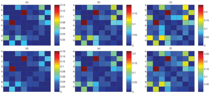
Results for Rochdale data—posterior means (second column), and 2.5 and 97.5 percentiles (first and third column, respectively) of the pairwise normalized mutual information matrix (top row) and the pairwise Cramer’s V association matrix (bottom row). (The online version of this figure is in color.)

The MCMC was also run with the set of 10 factors for the entire length of the chain with a beta(1, 1) prior on β. The results were robust, with the same ordering of the pairwise Cramer V’s obtained as in the previous case. As discussed before, the stick-breaking prior on the ${\nu }_h^{\ast }$ drives the ν_h’s for the redundant components close to zero, thereby making the procedure robust with respect to the choice of the number of factors as long as there are sufficiently many factors.

5. SIMULATION STUDY

We considered two simulation scenarios to assess the performance of the simplex factor model. We simulated y_ij ∈ {A, C, G, T} at p = 50 locations and a nominal response u_i having two and three levels in the two simulation cases, respectively. We considered two pure species (k = 2) and simulated the local subpopulation indices z_ij as in (9) to induce dependence among the response and a subset of locations J = (2, 4, 12, 14, 32, 34, 42, 44)^T. The eight locations in J had different A, C, G, T probabilities in the two pure species, while the phenotype probabilities at the remaining 42 locations were chosen to be the discrete uniform distribution on four points in each species.

In the first simulation scenario, we considered n = 100 sequences and two randomly chosen subpopulations of sizes 60 and 40, respectively. All the z_ij’s were assigned a value of 1 in the first subpopulation, and 2 in the second one. Within each subpopulation, the nucleotides were drawn independently across locations, with the jth nucleotide having phenotype probabilities ${({\lambda }_{z_{ij}A}^{(j)},{\lambda }_{z_{ij}C}^{(j)},{\lambda }_{z_{ij}G}^{(j)},{\lambda }_{z_{ij}T}^{(j)})}^{\text{T}}$. The binary response (u_i ∈ {1, 2}) had category probabilities (0.92, 0.08) and (0.08, 0.92) in the two subpopulations, respectively.

The second scenario had a more complicated dependence structure. We considered 200 sequences and three subpopulations of sizes 80, 80, and 40, respectively, with all the local indices z_ij assigned a value of 1 and 2, respectively, in the first two subpopulations. In the third subpopulation, the z_ij’s for the first 30 locations were assigned a value of 1 (z_ij = 1, j = 1, …, 30), and the remaining 20 locations a value of 2 (z_ij = 2, j = 31, …, 50). The response variable had three categories in this case, with category probabilities (0.90, 0.05, 0.05), (0.05, 0.90, 0.05), and (0.05, 0.05, 0.90) in the three subpopulations, respectively. The third subpopulation is biologically motivated as a rare group that has local similarities with each of the other groups, and thus, is difficult to distinguish from the other two.

For each case, we generated 50 simulation replicates and the simplex factor model was fitted separately to each dataset using the MCMC algorithm mentioned in Section 3.1. The sampler was run for 30,000 iterations, with a burn-in of 10,000 and every fifth sample was collected. We obtained good mixing and convergence for the elements of the pairwise mutual information matrix based on examination of trace plots. Figure 2 shows the posterior means of the pairwise normalized mutual information matrix m_jj′ averaged across simulation replicates in the two simulation scenarios, with the last row/column corresponding to the response variable. The posterior means corresponding to all $\left(\begin{array}{c}9\\ 2\end{array}\right)=36$ dependent location pairs are clearly well separated from the remaining nondependent pairs. We also provide kernel density plots of the posterior means and upper 97.5 percentiles of the m_jj′ across the 50 replicates for the two simulation cases in Figure 3. For the first simulation case (top row), the density plot for the posterior means in Figure 3(a) is bimodal, with a tall spike near zero and a very heavy right tail, thus showing a clear separation between the dependent and the nondependent pairs. The second simulation also had a very heavy tail for the posterior means in Figure 3(c), and the second mode is visible for the upper quantile in Figure 3(d).

Figure 2.

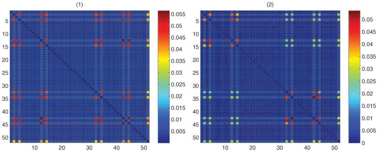
Simulation results—posterior means of the pairwise normalized information matrix of the nominal variables in simulation cases 1 and 2. Dependence between locations (2, 4, 12, 14, 32, 34, 42, 44) and the response (last row/column). (The online version of this figure is in color.)

Figure 3.

Simulation results—density plots of the posterior means (first column) and upper 97.5 percentiles (second column) of the p.w. normalized mutual information m_{jj ′}’s across simulation replicates in the two simulation cases.

Next, we aim to assess out-of-sample predictive performance for the simplex factor model. Since the subpopulations were chosen in a random order, we chose the first 20 samples in simulation case 1 and the first 30 samples in simulation case 2 as training sets within each replicate. We compared our approach with the Dunson and Xing (2009) method, a tree classifier built in MATLAB, and the random forest ensemble classifier (Breiman 2001), which was implemented using the RandomForest package (Liaw and Wiener 2002) in R. We did not consider a fully Bayesian graphical modeling approach, such as Dobra and Lenkoski (2011), because such methods do not scale computationally to the sized contingency tables we are considering. Figure 4 shows box plots of the overall and group-specific misclassification proportions for the different methods across the simulation replicates. As expected, the misclassification rates for simulation case 2 are higher than simulation case 1. The misclassification percentages corresponding to the second category are slightly larger than those for the first category in simulation case 1, which is explained by the relative sizes of the two subpopulations. It is clear from Figure 4 that the simplex factor model had better performance than the tree classifier and the random forest classifier in both cases. The overall misclassification percentage and category-specific misclassification percentages for the simplex factor model and random forest in the two simulation scenarios are provided in Table 1.

Figure 4.

Box plots for misclassification proportions across simulation replicates for the different methods. TREE = tree-based classifier, RF = random forest classifier, DX = Dunson–Xing method, SF = simplex factor model. The top row corresponds to simulation case 1, bottom row to simulation case 2. The first column corresponds to overall misclassification proportion, the remaining columns indicate group-specific misclassification proportions. (The online version of this figure is in color.)

Table 1.

Misclassification percentages in the two simulation cases for the simplex factor model and random forest

	Simulation case 1		Simulation case 2
	Simplex factor	Random forest	Simplex factor	Random forest
Best	(2.50, 0, 3.03)	(2.50, 0, 3.03)	(6.47, 1.54, 0, 8.10)	(8.82, 0, 0, 13.89)
Average	(7.55, 5.45, 10.39)	(9.90, 5.84, 15.51)	(14.08, 7.15, 6.80, 37.07)	(16.67, 9.30, 9.18, 41.03)
Worst	(16.25, 12.00, 28.57)	(35.00, 16.32, 77.77)	(34.12, 14.49, 13.89, 100)	(34.70, 27.14, 31.74, 100)

NOTE: Each vector represents overall and category-specific misclassification percentages, with the categories arranged according to their index. Best-, average-, and worst-case performances across replicates are reported.

Simulation case 1 was designed to comply with the Dunson and Xing (2009) model, since all of the variables for a particular subject were assigned to the same subpopulation. Accordingly, the Dunson and Xing (2009) method had very similar performance compared with the simplex factor model in the first case and did better than the other two methods. However, the performance of the Dunson and Xing (2009) method deteriorated in simulation case 2. In this case, the subjects in the third group had mixed membership for the different variables and the misclassification rates for this group were particularly high for the Dunson and Xing (2009) method.

6. NUCLEOTIDE SEQUENCE APPLICATIONS

We first applied our method to the p53 transcription factor-binding motif data (Wei et al. 2006). The data have n = 574 DNA sequences consisting of A, C, G, T nucleotides (d_j = 4) at p = 20 positions. Transcription factors are proteins that bind to specific locations within DNA sequences and regulate copying of genetic information from the DNA to them RNA. p53 is a widely known tumor suppressor protein that regulates expression of genes involved in a variety of cellular functions. It is of substantial biological interest to discover positional dependence within such DNA sequences.

We ran the MCMC algorithm for 25,000 iterations after the tuning phase, with a burn-in of 10,000 and collected every fifth sample. The adaptive algorithm selected four factors and we obtained acceptance rates greater than 90% for all the elements of ν^* using our proposed independence sampler. Using a gamma(0.1, 0.1) prior for α, the posterior mean of α was 0.11, with a 95% credible interval of (0.08–0.16). From Proposition 2.2, the small value of α indicates that the model favors a simpler dependence structure, as in Dunson and Xing (2009). We actually obtained very similar results to the Dunson and Xing (2009) method for this particular dataset. Figure 5(a)–(c) shows the posterior means and quantiles for the simplex factor model. Figure 5(d)–(f) shows the same for the Dunson and Xing (2009) method. Clearly, the dependence structure is sparse and the strongest dependence are found near the center of the sequence, with position pairs (11, 12) and (9, 11) having the largest normalized mutual information using both methods. The Xie and Geng (2008) approach flagged all 190 pairs as dependent using a p-value of 0.01 or 0.05 for edge inclusion; such overfitting can typically occur for Bayes Nets unless the threshold on edge inclusion is very carefully chosen.

Figure 5.

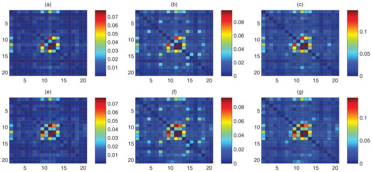
Results for the p53 data—posterior means (second column), and 2.5 and 97.5 percentiles (first and third column, respectively) of the normalized mutual information matrix. The top row corresponds to the simplex factor model, the bottom row is for the Dunson and Xing (2009) method. (The online version of this figure is in color.)

We next applied our method to the promoter data (Frank and Asuncion 2010) publicly available at the UCI Machine Learning Repository. The data consist of A, C, G, T nucleotides at p = 57 positions for n = 106 sequences, along with a binary response indicating instances of promoters and nonpromoters. There are 53 promoter sequences and 53 nonpromoter sequences in the dataset. We selected six training sizes as 20%, 30%, 40%, 50%, 60%, and 70% of the sample size n. For each training size, we randomly selected 10 training samples and evaluated the overall misclassification percentage and misclassification percentages specific to the promoter and nonpromoter groups. We compared out-of-sample predictive performance with the Dunson and Xing (2009) method, random forest, and a tree classifier. The MCMC algorithm for the simplex factor model was run for 30,000 iterations, with five factors selected. Our proposed approach for updating the ${\nu }_h^{\ast }$’s again produced high acceptance rates; the mean acceptance rates averaged across all replicates for ${\nu }_1^{\ast }-{\nu }_4^{\ast }$ were 0.85, 0.92, 0.96, and 0.97, respectively. The posterior means for α across all replicates within each training size was greater than 1; we have provided box plots for the posterior samples of α across the 10 replicates corresponding to the smallest training size in Figure 6.

Figure 6.

Results for the promoter data—box plots for posterior samples of α for the 10 replicates in the first case, where training size is 20% of the sample size. The red line denotes the posterior median, and the edges of the box denote posterior 25th and 75th percentiles. (The online version of this figure is in color.)

The simplex factor model had superior performance compared with the other three methods across all training sizes. In particular, for the training size = 20, the average misclassification percentages (overall, promoters, nonpromoters) for the Dunson and Xing (2009) method and random forest were (23.41, 26.24, 19.69) and (25.53, 29.92, 19.30), respectively, while the same for our method were (14.35, 15.41, 12.16). Table 2 provides the average-, best-, and worst-case misclassification percentages for the simplex factor model and random forest corresponding to the smallest and largest training sizes. From Table 2, the misclassification percentage for the nonpromoter group was smaller compared with that of the promoter group. For the smallest training size of 21, the simplex factor model provides an improvement of more than 14% in terms of the misclassification percentages for the promoter group. We also plot the average-, best-, and worst-case overall misclassification proportions across different training sizes for the competing methods in Figure 7 and the average misclassification proportions specific to the promoter and nonpromoter groups in Figure 8. It is clearly seen from Figures 7 and 8 that the simplex factor model provides the best performance across all training sizes.

Table 2.

Results for the promoter data—misclassification percentages (overall, among promoters, among nonpromoters) for the smallest and largest training sizes for the simplex factor model and random forest

	Training size = 21		Training size = 74
	Simplex factor	Random forest	Simplex factor	Random forest
Best	(8.24, 0, 0)	(15.29, 0, 0)	(0, 0, 0)	(6.25, 0, 0)
Average	(14.35, 15.41, 12.16)	(25.53, 29.92, 19.30)	(7.81, 10.14, 4.79)	(12.50, 17.84, 6.37)
Worst	(30.59, 53.32, 35.56)	(44.71, 80.85, 64.44)	(15.62, 21.05, 17.65)	(15.62, 33.33, 23.53)

NOTE: Best-, average-, and worst-case performances across 10 training samples for each training size are reported.

Figure 7.

Results for the promoter data—misclassification proportions (overall) for the different methods versus training size (ranging from 20% to 70% of the sample size n = 106). The rows correspond to average-, worst- and best-case performances, respectively, across 10 training sets for each training size. (The online version of this figure is in color.)

Figure 8.

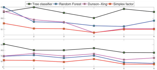
Results for the promoter data—average misclassification proportions (for the promoter and nonpromoter group, respectively) for the different methods versus training size (ranging from 20% to 70% of the sample size n = 106). (The online version of this figure is in color.)

We performed sensitivity analysis for the prior on α by choosing a gamma(1, 1) prior instead of gamma(0.1, 0.1), with the results unchanged. We also multiplied and divided the prior mean by a factor of 2 and did not observe any notable changes. For ${\nu }_h^{\ast }$, the uniform prior was found to be a reasonable default choice, as in most practical cases, one expects to have few dominant components in the case of contingency tables. That said, one can alternatively place a beta(1, β) prior on ${\nu }_h^{\ast }$, with a gamma prior assigned to β.

The additional flexibility of our model over the nonparametric Bayes method of Dunson and Xing (2009) produces improved performance in classification for the promoter data, and our approach also does better than sophisticated frequentist methods such as the tree classifier and random forest. We also applied our classification method to the splice data (publicly available at the UCI Machine Learning Repository) and obtained similar conclusions.

7. DISCUSSION

In a variety of problems, one now encounters data where the dimensionality of the outcome is comparable or even larger than the number of subjects. In such scenarios, one needs to make sparsity assumptions for meaningful inference. For continuous outcomes, one might consider sparse modeling of the covariance matrix via factor models or alternatively use Gaussian graphical models for sparse modeling of the precision matrix. However, the scope of either of these two frameworks is not solely limited to continuous variables. In more general terms, graphical models aim to model conditional dependencies among the variables, while factor models model marginal dependence relationships. In this article, we have proposed a sparse Bayesian factor modeling approach for multivariate nominal data that aims to explain dependence among high-dimensional nominal variables in terms of few latent factors that reside on a simplex. Posterior computation is straightforward and scales linearly with n and p. The proposed method can be thus used in high-dimensional problems, which is an advantage over graphical model-based approaches, which face computational challenges in scaling up to high dimensions.

An interesting extension of our proposed approach is joint modeling of a vector of nominal predictors and a continuous response, and more generally mixtures of different data types, as such situations are often encountered in biological and social sciences. To elaborate, let y_i = (y_i1, …, y_ip)^T denote a vector of observations as before, where the y_ij’s now are allowed to be of different types, such as binary, count, ordinal, continuous, etc. Letting γ_i = (γ_i1, …, γ_ip)^T ∈ {1, 2, …,∞}^p denote a multivariate latent class index for subject i, one can let

$$y_{ij}~{\mathcal{K}}_j({\theta }_{{\gamma }_{ij}j}),j=1,\dots ,p,{\gamma }_i~G,G~\mathrm{\Pi },$$ (16)

where G is the joint distribution of the multivariate categorical variable γ_i. The different y_ij’s are assumed to be conditionally independent, given the latent class index γ_i, and a prior Π on the distribution G of the latent class indices induces dependence among the y_ij’s. In a Dirichlet process mixture modeling framework, one usually has a single cluster index γ_i for the different data types, which forces individuals to be allocated to the same cluster across all data types. This often leads to blowing up of the number of clusters and degraded performance; see, for example, Dunson (2009). We can instead allow for separate but dependent clustering across the different domains by letting Π correspond to the simplex factor prior. One can also include covariate information by stacking together the covariates x_i and the response y_i in a vector z_i = (y_i, x_i) and jointly model z_i as above, with inference based on the induced conditional distribution of y_i | x_i obtained from the joint model. Müller, Erkanli, and West (1996) considered such joint models in a nonparametric Bayes frame work using Dirichlet process mixtures.

There has been a recent surge of interest in developing flexible Bayesian density regression models where the entire conditional distribution of the response y, given the predictors x, is allowed to change flexibly with x; see, for example, Griffin and Steel (2006); Dunson, Pillai, and Park (2007); Dunson and Park (2008); Chung and Dunson (2009); Rodriguez and Dunson (2011). It would be interesting to consider extensions of these models for multivariate categorical response variables by allowing predictor-dependent weights, for example, using the probit stick-breaking process (Chung and Dunson 2009; Rodriguez and Dunson 2011). Pati and Dunson (2011) developed theoretical tools for studying posterior consistency with a broad class of predictor-dependent stick-breaking priors; see also Norets and Pelenis (2011). Along those lines, one can envision extensions of our baseline posterior consistency results to the uncountable collection of probability tensors {π(x): x ∈ }.

APPENDIX

Proof of Proposition 2.2

From Equation (10), one has

$$g_{h_1\dots h_p}=\frac{{\prod }_{h:{\tau }_h\ne 0}(\alpha {\nu }_h)(\alpha {\nu }_h+1),\dots ,(\alpha {\nu }_h+{\tau }_h-1)}{\alpha (\alpha +1),\dots ,(\alpha +p-1)}.$$

Dividing the numerator and the denominator in the above expression by α^p, it is evident that ${lim}_{\alpha \to \infty }{g}_{h_1,\dots ,h_p}={\mathrm{\Pi }}_{h=1}^k{\nu }_h^{{\tau }_h}={\nu }_{h_1},\dots ,{\nu }_{h_p}$, which corresponds to the product multinomial model.

On the other hand,

$$g_{h\dots h}=\frac{(\alpha {\nu }_h)(\alpha {\nu }_h+1),\dots ,(\alpha {\nu }_h+p-1)}{\alpha (\alpha +1),\dots ,(\alpha +p-1)}.$$

Clearly, lim_α→0 g_h…h = ν_h, and thus in the limit, ${\sum }_{h=1}^k{g}_{h\dots h}=1$. As G is a probability tensor for every value of α, the nondiagonal elements must converge to 0 as α → 0. Hence, in this limiting case, G becomes super-diagonal and thus corresponds to the Dunson and Xing (2009) model.

Proof of Theorem 2.3

Fix π⁰ ∈ Π_d1…dp and ε > 0. For π ∈ Π_d1…dp, the L₁ distance between π and π⁰ is defined as

$${\left|\right|\mathit{\pi }-{\mathit{\pi }}^0\left|\right|}_1=\sum _{c_1=1}^{d_1}\dots \sum _{c_p=1}^{d_p}\mid {\pi }_{c_1\dots c_p}-{\pi }_{c_1\dots c_p}^0\mid .$$

Suppose π⁰ has nonnegative PARAFAC rank k, so π⁰ can be expressed as:

$${\mathit{\pi }}^0=\sum _{h=1}^k{\nu }_{0h}{\mathbf{\Lambda }}_{0h},{\mathbf{\Lambda }}_{0h}={\mathbf{\lambda }}_{0h}^{(1)}\otimes \cdots \otimes {\mathbf{\lambda }}_{0h}^{(p)},$$

where ν₀ ∈ and ${\mathbf{\lambda }}_{0h}^{(1)},\dots ,{\mathbf{\lambda }}_{0h}^{(p)}$ are probability vectors of dimensions d₁, …, d_p for each h ∈ {1, …, k}. The prior probability assigned to an ε-sized L₁-neighborhood (π⁰) of π⁰ by a k-component simplex factor model is given by:

$$\begin{array}{l}{\mathcal{Q}}_{\pi }^{(k)}\{{\mathcal{N}}_{\epsilon }({\mathit{\pi }}^0)\}=\int 1({\left|\right|\mathit{\pi }-{\mathit{\pi }}^0\left|\right|}_1<\epsilon )\\ d{\mathcal{Q}}_{\pi }^{(k)}(\mathit{\nu },\alpha ,{\mathbf{\lambda }}_h^{(j)},h=1,\dots ,k;j=1,\dots ,p),\end{array}$$ (A.1)

where

$${\pi }_{c_1\dots c_p}=\sum _{h_1=1}^k\dots \sum _{h_p=1}^k{g}_{h_1\dots h_p}\prod _{j=1}^p{\lambda }_{h_j{c}_j}^{(j)},$$

with g_h1…hp, as in Equation (10). Using Proposition 2.2 and standard algebra, it can be shown that for any ε > 0, there exist α̃ > 0 and ε̃ > 0 such that

$$\alpha <\stackrel{\sim }{\alpha },{\left|\right|\mathit{\nu }-{\mathit{\nu }}_0\left|\right|}_1<\stackrel{\sim }{\epsilon },{\Vert {\mathbf{\lambda }}_h^{(j)}-{\mathbf{\lambda }}_{0h}^{(j)}\Vert }_1<\stackrel{\sim }{\epsilon }\forall h,j$$

implies that ||π − π⁰||₁ < ε. Hence, to prove that (A.1) is positive, it suffices to show that 12501000:

$${\mathcal{Q}}_{\pi }^{(k)}(\alpha <\stackrel{\sim }{\alpha },{\left|\right|\mathit{\nu }-{\mathit{\nu }}_0\left|\right|}_1<\stackrel{\sim }{\epsilon },{\Vert {\mathbf{\lambda }}_h^{(j)}-{\mathbf{\lambda }}_{0h}^{(j)}\Vert }_1<\stackrel{\sim }{\epsilon },h=1,\dots ,k;j=1,\dots ,p)>0,$$

which immediately follows from the prior specification in (9).

Updating ν

We drop the h superscript in $c_l^{(h)}$ for notational convenience. Let

$$f({\nu }_h^{\ast })=\prod _{i=1}^n\prod _{l=h}^k\frac{\mathrm{\Gamma }(\alpha {\nu }_l+m_{il})}{\mathrm{\Gamma }(\alpha {\nu }_l)}=\left[\prod _{i:m_{ih}\ne 0}\frac{\mathrm{\Gamma }(c_h{\nu }_h^{\ast }+m_{ih})}{\mathrm{\Gamma }(c_h{\nu }_h^{\ast })}\right]\times \left[\prod _{l=h+1}^k\prod _{i:m_{il}\ne 0}\frac{\mathrm{\Gamma }\{c_l(1-{\nu }_h^{\ast })+m_{il}\}}{\mathrm{\Gamma }\{c_l(1-{\nu }_h^{\ast })\}}\right]$$ (A.2)

denote the unnormalized conditional posterior, and define $\phi ({\nu }_h^{\ast })=logf({\nu }_h^{\ast })$. When m_h > 0 and m_h+ = 0,

$$\pi ({\nu }_h^{\ast }\mid -)\propto \prod _{i:m_{ih}\ne 0}\prod _{s=0}^{m_{ih}-1}(c_h{\nu }_h^{\ast }+s),$$

so ${lim}_{{\nu }_h^{\ast }\to 0}\pi ({\nu }_h^{\ast }\mid -)=0,0<{lim}_{{\nu }_h^{\ast }\to 1}\pi ({\nu }_h^{\ast }\mid -)<\infty$, and $\pi ({\nu }_h^{\ast }\mid -)$ is convex. Similarly, if m_h = 0 and m_h+ > 0, then $0<{lim}_{{\nu }_h^{\ast }\to 0}\pi ({\nu }_h^{\ast }\mid -)<\infty ,{lim}_{{\nu }_h^{\ast }\to 1}\pi ({\nu }_h^{\ast }\mid -)<0$, and $\pi ({\nu }_h^{\ast }\mid -)$ is convex. In both these cases, the conditional posterior of ${\nu }_h^{\ast }$ can be approximated by a single beta density.

When m_h > 0 and m_h+ > 0,

$$\begin{array}{l}\phi ({\nu }_h^{\ast })=\sum _{l=h}^k\sum _{i:m_{il}\ne 0}\sum _{s=0}^{m_{il}-1}log(\alpha {\nu }_l+s)\\ =\sum _{l=h}^k\sum _{s=0}^{\infty }log(\alpha {\nu }_l+s)n_{ls}=\sum _{s=0}^{\infty }{n}_{hs}log(c_h{\nu }_h^{\ast }+s)+\sum _{s=0}^{\infty }\sum _{l=h+1}^k{n}_{ls}log\{c_l(1-{\nu }_h^{\ast })+s\}.\end{array}$$

As ${\nu }_h^{\ast }\to 0,{\sum }_{s=1}^{\infty }{n}_{hs}log(c_h{\nu }_h^{\ast }+s)+{\sum }_{s=0}^{\infty }{\sum }_{l=h+1}^k{n}_{ls}log\{c_l(1-{\nu }_h^{\ast })+s\}$ converges to a finite limit. Since m_h > 0, n_h0 > 0 and thus ${lim}_{{\nu }_h^{\ast }\to 0}{n}_{h0}log(c_h{\nu }_h^{\ast })=-\infty$, implying ${lim}_{{\nu }_h^{\ast }\to 0}\phi ({\nu }_h^{\ast })=-\infty$. Similarly, ${lim}_{{\nu }_h^{\ast }\to 1}\phi ({\nu }_h^{\ast })=-\infty$, since m_h+ > 0 implies that there exists h′ > h such that n_h′s > 0. Hence, ${lim}_{{\nu }_h^{\ast }\to 0,1}\phi ({\nu }_h^{\ast })=-\infty$ and thus ${lim}_{{\nu }_h^{\ast }\to 0,1}\pi ({\nu }_h^{\ast }\mid -)=0$.

We now show that $\pi ({\nu }_h^{\ast }\mid -)$ has a unique mode by considering the first and second derivatives of φ. We have

$${\phi }^{\prime }({\nu }_h^{\ast })=\sum _{s=0}^{\infty }{n}_{hs}\frac{c_h}{(c_h{\nu }_h^{\ast }+s)}-\sum _{s=0}^{\infty }\sum _{l=h+1}^k{n}_{ls}\frac{c_l}{\{c_l(1-{\nu }_h^{\ast })+s\}},$$ (A.3)

and

$${\phi }^{″}({\nu }_h^{\ast })=-\sum _{s=0}^{\infty }{n}_{hs}{\left\{\frac{c_h}{(c_h{\nu }_h^{\ast }+s)}\right\}}^2-\sum _{s=0}^{\infty }\sum _{l=h+1}^k{n}_{ls}{\left\{\frac{c_l}{\{c_l(1-{\nu }_h^{\ast })+s\}}\right\}}^2.$$ (A.4)

Once again, using the fact that n_h0 > 0 and there exists h′ > h such that n_h′0 > 0, one can prove that ${lim}_{{\nu }_h^{\ast }\to 0}{\phi }^{\prime }({\nu }_h^{\ast })=\infty$ and ${lim}_{{\nu }_h^{\ast }\to 1}{\phi }^{\prime }({\nu }_h^{\ast })=-\infty$. One can then find ε > 0 such that ${\phi }^{\prime }({\nu }_h^{\ast })>0$ for ${\nu }_h^{\ast }<\epsilon$ and ${\phi }^{\prime }({\nu }_h^{\ast })<0$ for ${\nu }_h^{\ast }>1-\epsilon$. Since φ′ is a continuous function, by the intermediate value theorem, there exists ${\nu }_{0h}^{\ast }\in (0,1)$ such that ${\phi }^{\prime }({\nu }_{0h}^{\ast })=0$. Since ${\phi }^{″}({\nu }_h^{\ast })<0$ on (0, 1), φ′ is monotonically decreasing and hence ${\nu }_{0h}^{\ast }$ is the unique mode of $\pi ({\nu }_h^{\ast }\mid -)$.

Next, we discuss an approach to avoid the grid approximation and obtain analytic expressions for the parameters of the approximating beta distribution. When m_h > 0 and m_h+ = 0, we want to find a ≥ 1 such that a beta(a, 1) approximates $\pi ({\nu }_h^{\ast }\mid -)$. Define $\stackrel{\sim }{f}({\nu }_h^{\ast })=f({\nu }_h^{\ast })/f(1)$ so that f̃(1) = 1. Hence, the above problem can be equivalently posed as approximating $\stackrel{\sim }{f}({\nu }_h^{\ast })$ by ${({\nu }_h^{\ast })}^{a-1}$. Since ${\int }_0^{1}log\{{({\nu }_h^{\ast })}^{a-1}\}d{\nu }_h^{\ast }=-(a-1)$, we let $\widehat{a}=1-{\int }_0^1\stackrel{\sim }{\phi }({\nu }_h^{\ast })d{\nu }_h^{\ast }$, where φ(x) = log f̃(x), which leads to the expression in (14). Observe that log(1 + c_h/s) ≤ c_h/s; hence, â ≥ 1. The analysis for the case where m_h = 0 and m_h+ > 0 proceeds along similar lines, where we define $\stackrel{\sim }{f}({\nu }_h^{\ast })=f({\nu }_h^{\ast })/f(0)$ and find b̂ so that $\stackrel{\sim }{f}({\nu }_h^{\ast })\approx {(1-{\nu }_h^{\ast })}^{b-1}$.

When m_h > 0 and m_h+ > 0, the analysis proceeds slightly differently. We want a, b ≥ 1 such that $\pi ({\nu }_h^{\ast }\mid -)\approx \{1/\text{beta}(a,b)\}{({\nu }_h^{\ast })}^{a-1}{(1-{\nu }_h^{\ast })}^{b-1}$. Comparing the first three moments of $log\pi ({\nu }_h^{\ast }\mid -)$ to the log beta(a, b) density, we build the 2 × 2 linear system mentioned in Section 3.1 to estimate a, b. The formulas for d₁, d₂ can be obtained from the following expressions

$$\begin{array}{l}{\int }_0^{1}log\pi ({\nu }_h^{\ast }\mid -)d{\nu }_h^{\ast }=logc+\sum _{s=0}^{\infty }\sum _{l=h}^k{n}_{ls}{\psi }_0(c_l,s)\\ {\int }_0^{1}2{\nu }_h^{\ast }log\pi ({\nu }_h^{\ast }\mid -)d{\nu }_h^{\ast }=logc+2\sum _{s=0}^{\infty }{n}_{hs}{\psi }_1(c_h,s)+2\sum _{s=0}^{\infty }\sum _{l=h+1}^k{n}_{ls}\{{\psi }_0(c_l,s)-{\psi }_1(c_l,s)\}\\ {\int }_0^{1}3{({\nu }_h^{\ast })}^{2}log\pi ({\nu }_h^{\ast }\mid -)d{\nu }_h^{\ast }=logc+3\sum _{s=0}^{\infty }\sum _{l=h}^k{n}_{ls}{\psi }_2(c_l,s)+3\sum _{s=0}^{\infty }\sum _{l=h+1}^k{n}_{ls}\{{\psi }_0(c_l,s)-2{\psi }_1(c_l,s)\},\end{array}$$

where

$$\begin{array}{l}{\psi }_0(c,s)={\int }_0^{1}log(cx+s)dx=\frac{s}{c}log(c+s)+log(c+s)-1-\frac{s}{c}log(s)\\ {\psi }_1(c,s)={\int }_0^{1}xlog(cx+s)dx=-\frac{s^2}{2c^2}log(c+s)+\frac{1}{2}log(c+s)+\frac{s}{2c}-\frac{1}{4}-\frac{s^2}{2c^2}log(s)\\ {\psi }_2(c,s)={\int }_0^1{x}^{2}log(cx+s)dx=\frac{s^3}{3c^3}log(c+s)+\frac{1}{3}log(c+s)-\frac{s^2}{3c^2}+\frac{s}{6c}-\frac{1}{9}-\frac{s^3}{3c^3}log(s).\end{array}$$

References

- Aitchison J, Bennett J. Polychotomous Quantal Response by Maximum Indicant. Biometrika. 1970;57(2):253–262. [Google Scholar]
- Ashford JR, Sowden RR. Multivariate Probit Analysis. Biometrics. 1970;26:535–546. [PubMed] [Google Scholar]
- Barnard K, Duygulu P, Forsyth D, De Freitas N, Blei D, Jordan M. Matching Words and Pictures. Journal of Machine Learning Research. 2003;3:1107–1135. [Google Scholar]
- Bishop Y, Fienberg S, Holland P. Discrete Multivariate Analysis: Theory and Practice. New York: Springer; 1975. [Google Scholar]
- Blei D, Ng A, Jordan M. Latent Dirichlet Allocation. Journal of Machine Learning Research. 2003;3:993–1022. [Google Scholar]
- Bollen K. Structural Equations With Latent Variables. New York: Wiley; 1989. [Google Scholar]
- Breiman L. Random Forests. Machine Learning. 2001;45(1):5–32. [Google Scholar]
- Carvalho C, Lucas J, Wang Q, Nevins J, West M. High-Dimensional Sparse Factor Modelling: Applications in Gene Expression Genomics. Journal of the American Statistical Association. 2008;103:1438–1456. doi: 10.1198/016214508000000869. [DOI] [PMC free article] [PubMed] [Google Scholar]
- Carvalho C, Scott J. Objective Bayesian Model Selection in Gaussian Graphical Models. Biometrika. 2009;96(3):1–16. [Google Scholar]
- Chib S, Greenberg E. Analysis of Multivariate Probit Models. Biometrika. 1998;85:347–361. [Google Scholar]
- Chung Y, Dunson D. Nonparametric Bayes Conditional Distribution Modeling With Variable Selection. Journal of the American Statistical Association. 2009;104(488):1646–1660. doi: 10.1198/jasa.2009.tm08302. [DOI] [PMC free article] [PubMed] [Google Scholar]
- Cohen JE, Rothblum UG. Nonnegative Ranks, Decompositions, and Factorizations of Nonnegative Matrices. Linear Algebra and Its Applications. 1993;190:149–168. [Google Scholar]
- Dawid A, Lauritzen S. Hyper Markov Laws in the Statistical Analysis of Decomposable Graphical Models. The Annals of Statistics. 1993;21(3):1272–1317. [Google Scholar]
- De Lathauwer L, De Moor B, Vandewalle J. A Multilinear Singular Value Decomposition. SIAM Journal on Matrix Analysis and Applications. 2000;21(4):1253–1278. [Google Scholar]
- Dobra A, Hans C, Jones B, Nevins J, Yao G, West M. Sparse Graphical Models for Exploring Gene Expression Data. Journal of Multivariate Analysis. 2004;90(1):196–212. [Google Scholar]
- Dobra A, Lenkoski A. Copula Gaussian Graphical Models. The Annals of Applied Statistics. 2011;5:969–993. [Google Scholar]
- Dobra A, Massam H. The Mode Oriented Stochastic Search (MOSS) Algorithm for Log-Linear Models With Conjugate Priors. Statistical Methodology. 2010;7(3):240–253. [Google Scholar]
- Dunson DB. Bayesian Latent Variable Models for Clustered Mixed Outcomes. Journal of the Royal Statistical Society, Series B. 2000;62(2):355–366. [Google Scholar]
- Dunson DB. Dynamic Latent Trait Models for Multidimensional Longitudinal Data. Journal of the American Statistical Association. 2003;98(463):555–563. [Google Scholar]
- Dunson DB. Nonparametric Bayes Local Partition Models for Random Effects. Biometrika. 2009;96(2):249. doi: 10.1093/biomet/asp021. [DOI] [PMC free article] [PubMed] [Google Scholar]
- Dunson DB, Park J. Kernel Stick-Breaking Processes. Biometrika. 2008;95(2):307. doi: 10.1093/biomet/asn012. [DOI] [PMC free article] [PubMed] [Google Scholar]
- Dunson DB, Pillai N, Park J. Bayesian Density Regression. Journal of the Royal Statistical Society, Series B. 2007;69(2):163–183. [Google Scholar]
- Dunson DB, Xing C. Nonparametric Bayes Modeling of Multivariate Categorical Data. Journal of the American Statistical Association. 2009;104(487):1042–1051. doi: 10.1198/jasa.2009.tm08439. [DOI] [PMC free article] [PubMed] [Google Scholar]
- Erosheva E, Fienberg S, Joutard C. Describing Disability Through Individual-Level Mixture Models for Multivariate Binary Data. The Annals of Applied Statistics. 2007;1(2):502–537. doi: 10.1214/07-aoas126. [DOI] [PMC free article] [PubMed] [Google Scholar]
- Ferguson TS. A Bayesian Analysis of Some Nonparametric Problems. The Annals of Statistics. 1973;1:209–230. [Google Scholar]
- Ferguson TS. Prior Distributions on Spaces of Probability Measures. The Annals of Statistics. 1974;2:615–629. [Google Scholar]
- Fienberg S, Rinaldo A. Three Centuries of Categorical Data Analysis: Log-Linear Models and Maximum Likelihood Estimation. Journal of Statistical Planning and Inference. 2007;137(11):3430–3445. [Google Scholar]
- Frank A, Asuncion A. UCI Machine Learning Repository. Irvine, CA: School of Information and Computer Science, University of California; 2010. available at http://archive.ics.uci.edu/ml. [Google Scholar]
- Ghosh J, Ramamoorthi R. Bayesian Nonparametrics. New York: Springer-Verlag; 2003. [Google Scholar]
- Goodman LA. Explanatory Latent Structure Assigning Both Identifiable and Unidentifiable Models. Biometrika. 1974;61:215–231. [Google Scholar]
- Gregory D, Pullman N. Semiring Rank: Boolean Rank and Nonnegative Rank Factorizations. Journal of Combinatorics, Information & System Sciences. 1983;8(3):223–233. [Google Scholar]
- Griffin J, Steel M. Order-Based Dependent Dirichlet Processes. Journal of the American Statistical Association. 2006;101(473):179–194. [Google Scholar]
- Harshman R. UCLA Working Papers in Phonetics. 1. Vol. 16. Los Angeles, CA: UCLA; 1970. Foundations of the PARAFAC Procedure: Models and Conditions for an ‘Explanatory’ Multi-Modal Factor Analysis; p. 84. [Google Scholar]
- Ishwaran H, James L. Gibbs Sampling Methods for Stick-Breaking Priors. Journal of the American Statistical Association. 2001;96(453):161–173. [Google Scholar]
- Jones B, Carvalho C, Dobra A, Hans C, Carter C, West M. Experiments in Stochastic Computation for High-Dimensional Graphical Models. Statistical Science. 2005;20(4):388–400. [Google Scholar]
- Kim Y, Choi S. Nonnegative Tucker Decomposition. Proceedings of the IEEE Conference on Computer Vision and Pattern Recognition, 2007—CVPR’07; 2007. pp. 1–8. [Google Scholar]
- Kolda T. Orthogonal Tensor Decompositions. SIAM Journal on Matrix Analysis and Applications. 2001;23(1):243–255. [Google Scholar]
- Lauritzen S. Graphical Models. Oxford: Oxford University Press; 1996. [Google Scholar]
- Lazarsfeld P, Henry N. Latent Structure Analysis. Boston, MA: Houghton Mifflin; 1968. [Google Scholar]
- Lenkoski A, Dobra A. Computational Aspects Related to Inference in Gaussian Graphical Models With the G-Wishart Prior. Journal of Computational and Graphical Statistics. 2011;20(1):140–157. [Google Scholar]
- Liaw A, Wiener M. Classification and Regression by Random Forest. R News. 2002;2(3):18–22. [Google Scholar]
- Lopes H, West M. Bayesian Model Assessment in Factor Analysis. Statistica Sinica. 2004;14(1):41–68. [Google Scholar]
- Madigan D, York J. Bayesian Graphical Models for Discrete Data. International Statistical Review. 1995;63(2):215–232. [Google Scholar]
- Massam H, Liu J, Dobra A. A Conjugate Prior for Discrete Hierarchical Log-Linear Models. The Annals of Statistics. 2009;37(6A):3431–3467. [Google Scholar]
- Moustaki I, Knott M. Generalized Latent Trait Models. Psychometrika. 2000;65(3):391–411. [Google Scholar]
- Müller P, Erkanli A, West M. Bayesian Curve Fitting Using Multivariate Normal Mixtures. Biometrika. 1996;83(1):67. [Google Scholar]
- Muthén B. Latent Variable Structural Equation Modeling With Categorical Data. Journal of Econometrics. 1983;22(1–2):43–65. [Google Scholar]
- Norets A, Pelenis J. Technical report. Princeton, NJ: Princeton University; 2011. Posterior Consistency in Conditional Density Estimation by Covariate Dependent Mixtures. [Google Scholar]
- Ochi Y, Prentice R. Likelihood Inference in a Correlated Probit Regression Model. Biometrika. 1984;71(3):531–543. [Google Scholar]
- Pati D, Dunson D. Working Paper. Durham, NC: Department of Statistical Science, Duke University; 2011. Posterior Consistency in Conditional Distribution Estimation. [DOI] [PMC free article] [PubMed] [Google Scholar]
- Pitt M, Chan D, Kohn R. Efficient Bayesian Inference for Gaussian Copula Regression Models. Biometrika. 2006;93(3):537–554. [Google Scholar]
- Pritchard J, Stephens M, Donnelly P. Inference of Population Structure Using Multilocus Genotype Data. Genetics. 2000;155(2):945. doi: 10.1093/genetics/155.2.945. [DOI] [PMC free article] [PubMed] [Google Scholar]
- Rodriguez A, Dunson D. Nonparametric Bayesian Models Through Probit Stick-Breaking Processes. Bayesian Analysis. 2011;6:145–178. doi: 10.1214/11-BA605. [DOI] [PMC free article] [PubMed] [Google Scholar]
- Sammel M, Ryan L, Legler J. Latent Variable Models for Mixed Discrete and Continuous Outcomes. Journal of the Royal Statistical Society, Series B. 1997;59(3):667–678. [Google Scholar]
- Sethuraman J. A Constructive Definition of Dirichlet Priors. Statistica Sinica. 1994;4(2):639–650. [Google Scholar]
- Shashua A, Hazan T. Non Negative Tensor Factorization With Applications to Statistics and Computer Vision. Proceedings of the 22nd International Conference on Machine Learning; 2005. p. 799. [Google Scholar]
- Teh Y, Jordan M, Beal M, Blei D. Hierarchical Dirichlet Processes. Journal of the American Statistical Association. 2006;101(476):1566–1581. [Google Scholar]
- Tucker L. Some Mathematical Notes on Three-Mode Factor Analysis. Psychometrika. 1966;31(3):279–311. doi: 10.1007/BF02289464. [DOI] [PubMed] [Google Scholar]
- Wang H, Ahuja N. Rank-R Approximation of Tensors: Using Image-as-Matrix Representation. Proceedings of the IEEE Conference on Computer Vision and Pattern Recognition, 2005—CVPR’05; 2005. pp. 346–353. [Google Scholar]
- Wei C, Wu Q, Vega V, Chiu K, Ng P, Zhang T, et al. A Global Map of p53 Transcription-Factor Binding Sites in the Human Genome. Cell. 2006;124(1):207–219. doi: 10.1016/j.cell.2005.10.043. [DOI] [PubMed] [Google Scholar]
- West M. Bayesian Factor Regression Models in the ‘Large p, Small n’ Paradigm. Bayesian Statistics. 2003;7(2003):723–732. [Google Scholar]
- Whittaker J. Graphical Models in Applied Multivariate Statistics. New York: Wiley; 1990. [Google Scholar]
- Xie X, Geng Z. A Recursive Method for Structural Learning of Directed Acyclic Graphs. Journal of Machine Learning Research. 2008;9:459–483. [PMC free article] [PubMed] [Google Scholar]
- Zhang X, Boscardin WJ, Belin TR. Sampling Correlation Matrices in Bayesian Models With Correlated Latent Variables. Journal of Computational and Graphical Statistics. 2006;15(4):880–896. [Google Scholar]
- Zhang X, Boscardin WJ, Belin TR. Bayesian Analysis of Multivariate Nominal Measures Using Multivariate Multinomial Probit Models. Computational Statistics & Data Analysis. 2008;52:3297–3708. doi: 10.1016/j.csda.2007.12.012. [DOI] [PMC free article] [PubMed] [Google Scholar]