

Abstract
Genome-wide binding assays can determine where individual transcription factors bind in the genome. However, these factors rarely bind chromatin alone, but instead frequently bind to cis-regulatory elements (CREs) together with other factors thus forming protein complexes. Currently there are no integrative analytical approaches that can predict which complexes are formed on chromatin. Here, we describe a computational methodology to systematically capture protein complexes and infer their impact on gene expression. We applied our method to three human cell types, identified thousands of CREs, inferred known and undescribed complexes recruited to these CREs, and determined the role of the complexes as activators or repressors. Importantly, we found that the predicted complexes have a higher number of physical interactions between their members than expected by chance. Our work provides a mechanism for developing hypotheses about gene regulation via binding partners, and deciphering the interplay between combinatorial binding and gene expression.
Chromatin immunoprecipitation followed by sequencing (ChIP-seq) (Johnson et al. 2007) is being routinely used to identify the genomic binding locations of individual transcription factors (TF) in a given cell population. However, accumulating evidence suggests that these TFs rarely bind chromatin alone (Gerstein et al. 2012); instead they bind together with other factors as protein complexes (Moorman et al. 2006; Ram et al. 2011) (e.g., Polycomb Repressive Complex 2 [PRC2], MYC/MAX TF network, AP1 complex, and more). The number and composition of protein complexes that assemble on chromatin is largely unknown. How many binding sites on the genome are occupied by protein complexes, how these sites are distributed relative to genomic features (e.g., promoters, intergenic regions), and how chromatin-bound TF complexes are involved in regulation of cell-type–specific gene expression are still unknown for most human cell types. Even the role that known chromatin-bound complexes may play in regulation gene expression (Goke et al. 2011; Ram et al. 2011; Yu et al. 2011; Lee et al. 2012) is also often not well defined.
In the present study, we describe a computational methodology based on nonnegative matrix factorization (NMF) and regression analysis that systematically captures potential protein complexes, identifies where they bind in the genome, and infers their impact on gene expression. We have applied this method to a large collection of TF binding data across three different human cell types from the Encyclopedia of DNA elements (ENCODE) Project (The ENCODE Project Consortium 2011): embryonic stem cells (H1 ESC), B-lymphoblastoid cells (GM12878), and erythrocytic leukemia cells (K562). We also included histone modifications (HMs) in our analyses in order to consider protein complexes binding and its effect on transcription in the broader context of the chromatin landscape.
NMF has been used in several biological applications (Brunet et al. 2004; Kim and Park 2007; Xu et al. 2009; Pu et al. 2011) because its nonnegativity constraint (see Methods) provides an intuitive and biologically interpretable decomposition of a multivariate data set and a natural way to cluster biological data (Brunet et al. 2004). This is unlike principal components analysis, where eigenvectors with negative sign loadings can be hard to interpret in the context of positively valued variables such as ChIP-seq read counts. Unlike other clustering methods (e.g., hierarchical clustering, k-means clustering), NMF enables soft clustering, which allows for a TF to belong to multiple complexes and a genomic region to be a binding site for multiple TFs. This type of clustering is important in the context of transcriptional regulation.
Several studies have performed integrative analysis of multiple ChIP-seq data sets in different organisms (Ouyang et al. 2009; Rye et al. 2011; Herrmann et al. 2012; Shen et al. 2012). However, only a few of these studies have explored how combinatorial binding leads to the assembly of protein complexes on chromatin, and they have either been limited only to a handful of TFs (Yu et al. 2011) or have focused uniquely on chromatin regulators (Ram et al. 2011). Importantly, our work differs from recent studies that have used large collections of ChIP-seq data sets to segment the genome (Ernst et al. 2011; Ernst and Kellis 2012; Hoffman et al. 2012) into regulatory regions like promoters, enhancers, and insulators (Barski et al. 2007; Cuddapah et al. 2009; Moqtaderi et al. 2010; Rada-Iglesias et al. 2011), in that we aim to discover what factors bind the regulatory regions as protein complexes. Other studies have also shown that TF binding (Ouyang et al. 2009; Cheng and Gerstein 2011; Cheng et al. 2012), HMs (Karlic et al. 2010; Cheng et al. 2012; Wang et al. 2012a), and recently even DNase I hypersensitive sites (Natarajan et al. 2012) can explain a fraction of gene expression variation, but none of them have directly modeled the impact of complexes on gene expression. Thus, currently there are no broadly used integrative analytical approaches that can systematically infer the impact of protein complexes on gene expression.
In this paper, we describe a computational approach that uses multiple ENCODE ChIP-seq data sets to recapitulate known chromatin-bound complexes and to predict novel ones. Our method allows exploring and deciphering the interplay between combinatorial TF binding and gene expression, and serves as a valuable resource for understanding the collective function and role of regulatory elements and the complexes that bind them. The proposed computational approach can also generate hypotheses involving chromatin organization and gene regulation via co-regulators and binding partners.
Results
Detecting cis-regulatory elements and protein complexes, and modeling their effect on gene expression
The primary goal of this study is to systematically predict potential chromatin-bound protein complexes and infer their impact on gene expression using NMF and regression analysis. We applied the methodology described here to ChIP-seq data sets for the Tier 1 human cell types in the ENCODE project (i.e., H1 ESC, GM12878, K562). In total for the three cell types 64 TFs and 11 HMs were included in this study (Supplemental Table 1).
We first detected peaks (Giannopoulou and Elemento 2011) for every available ChIP-seq experiment in each cell type (Supplemental Fig. 1). Then we merged peaks from all experiments into cis-regulatory elements (CREs): regions with enrichment in at least one data set (Fig. 1A).
Figure 1.

Modeling gene expression from combinatorial binding. (A) Peaks from multiple experiments (TFs, HMs) are merged into nonoverlapping CREs, within the same cell type. (B) For each CRE, the normalized reads intensity in each experiment is estimated. The RC matrix is then produced, representing the CREs in rows, and the reads' intensity profiles of different experiments in columns. NMF analysis is applied to the RC matrix, to group the M experiments of TFs and HMs into k complexes. NMF decomposes the RC matrix into the basis matrix and the mixture coefficient matrix. The basis matrix contains the coefficient of each CRE in a complex (also called complex score), while each complex represents a positive linear combination of the original read count variables for each experiment (coefficients matrix). (C) The CREs that occur within a fixed-range window around a TSS are estimated. Then, the complex scores and the proximity of the CREs to the TSS of a gene are integrated into a Binding Influence Score (BIS) between a protein complex and a gene. d0 is a constant used to specify the shape of the exponential function (see Methods). (D) The BIS values are used as predictors to assess the contribution of protein complexes to gene expression in regression models.
For each CRE, we quantified the normalized ChIP-seq reads density in every experiment in order to build a read count matrix (RC matrix), whose rows correspond to CREs and columns to ChIP-seq experiments (Fig. 1B) (see Methods). NMF analysis was then performed on the RC matrix to group the CREs into clusters. Each NMF cluster represents a positive linear combination of the original normalized read count variables associated with each ChIP-seq experiment. Consequently, every cluster reveals a binding pattern that represents a set of TFs simultaneously found by ChIP-seq at the same CRE and associated HMs. Thus, NMF clusters provide evidence for the existence of potential complexes with one or more TFs/HMs. In brief, we computationally infer chromatin-bound protein complexes from the clusters uncovered by NMF.
In the next step of the workflow, the CREs that occur within a 50-kb window around a RefSeq transcription start site (TSS) were identified and integrated the complex scores, estimated by NMF, with the proximity of the CREs to a TSS, to measure the influence of a complex on a gene (Fig. 1C; Tabach et al. 2007; Cheng et al. 2012). These influence scores were then used as explanatory variables to assess the contribution of a complex to gene expression (Fig. 1D) (see Methods).
A critical parameter in this workflow is the factorization rank for NMF, which defines the number of clusters used to approximate the original matrix, and therefore the number of predicted complexes. In order to decide whether a given rank decomposes the original matrix into meaningful clusters we used several quality criteria that have been previously proposed for this type of approach (Brunet et al. 2004) (see Methods). In particular, we used different rank values, ranging from 2 to 20, estimated for each rank several quantitative measures, such as the cophenetic correlation and dispersion coefficients, and identified local maxima in these coefficients at high-rank factorization, in order to find complexes with high granularity (Supplemental Fig. 1). Additionally we used the consensus matrices visualization to help us find the ranks at which the NMF run shows robust clustering results (see Methods and Supplemental Figs. 2–4). We then performed NMF at these ranks (see Methods for the parameters and criteria used) to uncover the corresponding protein complexes. Finally, for each complex we extracted its most contributing CREs. The term complex-specific CREs mentioned in the following sections indicates these CREs, which contribute most in each of the discovered complexes.
Nonnegative matrix factorization identifies known protein complexes and predicts potential novel ones
After peak detection and merging of the overlapping peaks into CREs, we identified ∼100,000 CREs per cell type. These CREs were distributed in promoter, distal, intergenic, intronic, exonic, and downstream regions of genes, as shown in Figure 2A, and covered 7%–8% of the human genome (Supplemental Table 2). Additionally, we found that overall genes whose promoters were occupied by any of these CREs showed significantly higher expression than genes not occupied by them, across all cell types (Fig. 2B); this shows the functional significance of the identified CREs. Using pairwise Jaccard similarity coefficient (see Methods) between CREs of the three cell types, we also observed that the three cell types showed only ∼25% overlap between their CREs (Fig. 2C), which supports a cell-type–specific character of the detected elements. Importantly, almost half of these CREs were bound by more than one TF, suggesting that the CREs are possibly regions where multiple TFs assemble as protein complexes (Supplemental Fig. 5). Since we envision that TFs may either bind to chromatin alone in specific contexts (our analysis allows a TF to participate in multiple contexts) or with other co-factors not assayed by ChIP-seq, we did not filter out in CREs bound by only one TF in the present analysis. However, in the Supplemental Material we also show the complexes identified after filtering out the single TF-bound CREs and keeping only the CREs bound by at least two TFs (Supplemental Figs. 6, 7).
Figure 2.

Analysis of the CREs of three human cell types. (A) Genomic distribution of CREs and categorization in promoters (±2 kb around TSS), downstream extremities (±2 kb around TES), exons, introns, distal (>2 kb and <50 kb), and intergenic regions (>50 kb). CREs span multiple genomic regions in a fashion that agrees with the fraction of the human genome (hg19) in the above categories. (B) Boxplots showing that genes with CREs in their promoters (±2 kb around TSS) have significantly higher expression than genes not occupied by them, across all cell types. The y-axis shows absolute transcript expression levels measured by FPKM (fragments per kilobase of exon per million fragments mapped). P-values were calculated by Wilcoxon rank sum test. Three asterisks (***) indicate P-value < 2.2 × 10⁻¹⁶. (C) The Jaccard similarity coefficients are shown, indicating how similar the CREs are across the three cell types. The larger the coefficient, the more similar two peak sets are in terms of overlapping regions. Low coefficients of similarity are observed between the three cell types, supporting a cell-type–specific character of the detected CREs.
Local maxima in the cophenetic correlation and dispersion coefficients pointed to the existence of 17, 20, and 17 NMF clusters for H1 ESC, GM12878, and K562, respectively (Supplemental Figs. 1–4). Heatmaps showing the NMF clusters identified in each cell type are shown in Figure 3A. In each heatmap, rows correspond to TFs and HMs and columns to clusters. The rows of the heatmaps are ordered, and groups of TFs and HMs are color-coded in five groups, indicating common TFs in all three cell types (light red), common between H1 ESC and GM12878 only (light blue), common between GM12878 and K562 only (light yellow), common between H1 ESC and K562 only (light purple), and common HMs in all three cell types (light gray). TFs and HMs that are not highlighted depict data sets available only for the corresponding cell type (at the time of submission). The strength of each TF and HM in each cluster is shown using a color scale with dark red representing the strongest enrichment. Factorization at lower rank levels is presented in the Supplemental Material.
Figure 3.

Predicted complexes in three human cell types. (A) The heatmaps visualize the NMF coefficients matrices for the three cell types. (Columns) The detected complexes; (rows) the reads density binding pattern of the corresponding TF/HM experiment for each complex. The rows of the heatmaps are ordered, and groups of TFs and HMs are color-coded in five groups, indicating common TFs in all three cell types (light red), common between H1 ESC and GM12878 only (light blue), common between GM12878 and K562 only (light yellow), common between H1 ESC and K562 only (light purple), and common HMs in all three cell types (light gray). TFs and HMs that are not highlighted depict data sets available only for the corresponding cell type (at the time of submission). The cells depict the relative contribution of each complex to an experiment. All experiments are shown on the left of the heatmaps (HMs red, TFs blue). The TFs whose corresponding complex coefficient is >0.3 (and represent on average the top 5% of the NMF coefficients matrixes) are shown below each complex. These factors were strictly considered as complex members only for the protein–protein interaction analysis. (B) Genomic distribution of the complex-specific CREs and categorization in promoters (±2 kb around TSS), downstream extremities (±2 kb around TES), exons, introns, distal (>2 kb and <50 kb), and intergenic regions (>50 kb). (C) Regulatory motif analysis revealed the most enriched motifs for the complex-specific CREs. The z-scores for each predicted motif appears in parentheses. The motif logos are shown in Supplemental Figure 3. (D) The linear regression coefficients for each complex. The size of the coefficient corresponds to the size of the effect that each complex has on gene expression, and the sign of the coefficient (positive or negative) gives the direction of the effect. Statistical significance of the estimated coefficients is coded as: (***) 0 < P < 0.001; (**) 0.001 < P < 0.01; (*) 0.01 < P < 0.05; (•) 0.05 < P < 0.1; no value, 0.1 < P < 1.
A number of observations suggest that our method accurately recovers groups of functionally related chromatin-binding factors and that these factors are indeed involved in physical interactions compatible with protein complexes. In what follows, we use the notation H/G/K followed by a number to refer to the corresponding cluster in H1 ESC, GM12878, and K562 cell lines, respectively (Fig. 3A).
First, preliminary examination of the predicted protein complexes showed that complexes known to bind to and function at enhancers, such as the “enhanceosome” complex (Kim et al. 2008; Yu et al. 2011), or contain enhancer-related factors (e.g., EP300, SPI1) were frequently found in distal and intergenic regions rather than in promoters (H-11, G-4, G-11) (orange and light blue bars in Fig. 3B). The opposite was observed for complexes related to transcription initiation (e.g., complexes with TAF1) or promoter marks (e.g., H3K4me2, H3K4me3, H3K27me3, H3K79me2; H-4, H-7, H-9, K-2, K16) (dark blue bars in Fig. 3B).
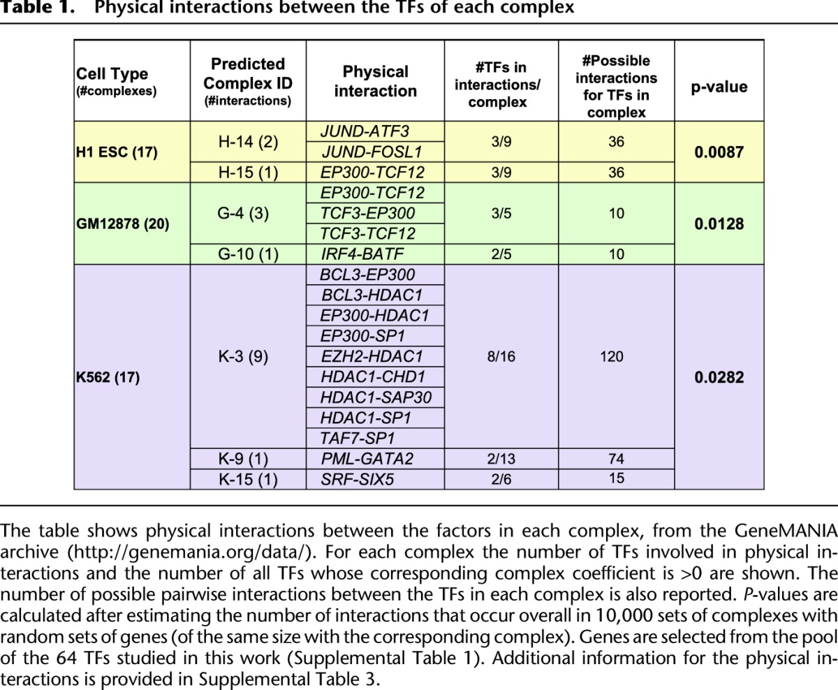
Second, we found that many of the members of the predicted complexes are involved in physical interactions as documented in the GeneMANIA (Warde-Farley et al. 2010) database (see Methods). In particular, using randomizations that involved generating random groups of TFs of the same size as the predicted ones by randomly combining genes from the pool of the 64 TFs studied in this work, we found that our predicted protein complexes are engaged more frequently in physical interactions than expected by chance (P < 0.01 in H1 ESC, P < 0.02 in GM12878, P < 0.03 in K562) (Table 1; Supplemental Table 3).
Table 1.
Physical interactions between the TFs of each complex
Third, several of the complexes identified in this study have been characterized before, partially or entirely. For example, our method predicted an EP300–TCF12 complex in two cell types (H-15, G-4); these two factors are known to physically interact (Table 1; Supplemental Table 3) and represent the previously described HEB/EP300 complex (TCF12 is also known as HEB) that has been reported in neuronal and T cells (D'Apuzzo et al. 2001; Zhang et al. 2004). We used regulatory motif analysis to search for overrepresented DNA motifs within the complex-specific CREs, in order to identify sequence-specific TFs likely to target the complexes to the chromatin (Fig. 3C; Supplemental Fig. 8). Motif analysis identified the TCF12 motif as overrepresented in the CREs of H-15, which indicates that TCF12 binds to DNA and recruits co-activators such as EP300 (O'Neil and Look 2007). Predicted complex H-14, which consists of ATF3–JUND–FOSL1 factors, is also well supported by the literature: JUND and FOSL1 are subunits of the well-characterized AP-1 complex, while ATF3 is known to interact with JUND (Table 1; Supplemental Table 3; Pearson et al. 2003). De novo motif analysis identified the consensus motif for AP-1 as enriched within the corresponding CREs, and not for CREB that is the canonical motif for the TF family that ATF3 belongs to, suggesting that AP-1 members bind to DNA and recruit ATF3 (Fig. 3C).
Other complexes identified using our approach are also known but include novel predicted subunits. For example, complex H-11 in Figure 3 contains the pluripotency factors NANOG–POU5F1–EP300, which are members of the “enhanceosome,” an EP300 histone acetyltranferase-recruiting complex (Kim et al. 2008; Yu et al. 2011). The corresponding CREs mostly occupied intergenic regions (∼60%), while only the SOX2–POU5F1 motif was identified as overrepresented (Fig. 3C). BCL11A, a zinc-finger protein that functions as a myeloid and B-cell proto-oncogene (Nakamura et al. 2000), and was recently found to be co-associated with NANOG in human stem cells (The ENCODE Project Consortium 2012), was also found in this complex.
The binding cluster of RBBP5–KDM5B–PHF8–HEY1–TAF1 was predicted in K-14, and was characterized by preferential binding in promoters (∼90%) (Fig. 3B). Interestingly, we were able to capture this binding combination that has also been reported in a recent study (together with the factors CHD1–SAP30–HDAC1 that are also found in K-14 with coefficients <0.3), where chromatin regulators were detected using a ChIP-based meso-scale assay (Ram et al. 2011). Our analysis also predicted HEY1 and TAF1 as additional members of the complex and potential binding partners of RBBP5, KDM5B, PHF8, CHD1, SAP30, and HDAC1. Complex K-3 in Figure 3 is another complex that contained EZH2, a PRC2 complex component, and HDAC1, a gene that PRC2 is known to interact with for transcriptional silencing (van der Vlag and Otte 1999). Complex K-3 was also associated with H3K27me3, which is catalyzed by EZH2. The majority of the K-3 complex-specific CREs occupied intergenic regions (∼76%), while only a small percentage occurred in promoters (2.8%). This could be explained by the presence of EP300 that is known to bind to enhancer elements (Visel et al. 2009). Other factors in the predicted complex include BCL3, CHD1, SAP30, SP1, SP2, TAF7, and ZBTB33; several known physical interactions occur among them such as BCL3–EP300, BCL3–HDAC1, EP300–SP1, CHD1–HDAC1, SAP30–HDAC1, SP1–HDAC, TAF7–SP1 (Table 1; Supplemental Table 3). We hypothesize that these factors may indicate co-regulators that interact with PRC2 via its subunits.
Importantly, our approach also made a number of novel predictions. One of these new complexes is ATF3–USF1 and was predicted in all cell types (H-6, G-13, K-5), with ∼27%–29% of its binding occurring in intergenic regions and only 2%–5% in promoters. The consensus sequence for an E-box element was found enriched in the complexes in both cell types (5′-CANNTG-3′), which is justified by the presence of USF1, a helix–loop–helix family member that can activate transcription through binding to E-box motifs (Fig. 3C; Rada-Iglesias et al. 2008). Since only USF1 motif was found enriched in the CREs of these potential complexes, we hypothesize that USF1 binds to DNA and recruits ATF3. A parallel study (Wang et al. 2012b) very recently also discovered that ATF3 tethers USF1, which binds to DNA. Similarly, in the corresponding CREs of the PBX3–SP1 complex (G-9) the DNA motif of NFYA factor was enriched, which is known to interact with SP1 (Roder et al. 1999). Although NFYA ChIP-seq data were not included in the NMF analysis, the discovery of the NFYA motif suggests that SP1 binds through or with NFYA to the DNA and consequently recruits PBX3. Finally, even though REST did not co-localize with other factors in H1 ESC and GM12878, the CTCF–REST complex was found in K562 (K-13). The motif for REST, and not CTCF, was enriched in the corresponding CREs, suggesting that REST might bind to the DNA in that cell line and recruit CTCF.
Other predicted protein complexes include: GABPA–SIN3A–KDM5B (H-2), SP1–SP2 (H-5), ELF1–EGR1–USF1 (G-2), PBX3–BCL3 (G-5), ETS1–ZBB7A (K-1), GABPA–SP2 (K-16), as well as BATF–IRF4 (G-10). The latter complex is indeed supported by a known physical interaction between BATF and IRF4 (Table 1; Supplemental Table 3; Ravasi et al. 2010). Most importantly, the predicted complexes captured by our method provide testable protein interaction hypotheses that could be further evaluated using techniques such as co-immunoprecipitation (Co-IP).
Finally, since a subset of TFs was present in all cell types (the 13 TFs shown at the top of the heatmaps in Fig. 3A), we sought to examine which complexes that include these TFs were common and which were different between the three cell types. As already mentioned, ATF3–USF1 was discovered in all three cell types (H-6, G-13, K-5), and ATF3–CTCF only in H1 ESC and GM12878 (H-3, G-1). REST did not co-localize with other factors in two cell types, but was clustered together with CTCF in K562 (K-13). SIX5 was clustered on its own in H1 ESC (H-17), but had different partners in GM12878 (G-8) and K562 (K-3, K-15). A similar pattern was observed for the factors YY1, TAF1, and SRF that did not co-localize with any other of the 13 common TFs in H1 ESC (H-10, H-4, and H-12, respectively), but had different partners in the other two cell types (G-3, K-15 for TAF1; G-3, G-13, and K-14 for YY1; G-2, G-6, K-3, K-12, and K-15 for SRF).
Protein complexes acting as activators or repressors
We next sought to predict the effect of these complexes on gene expression, and determine their role as activators or repressors. We thus used regression analysis in order to model and describe the mRNA expression levels of the genes in a given cell type as a function of the protein complexes binding near the genes (Fig. 1C,D). We developed two regression models, a linear model using ordinary least squares linear regression, as well as a nonlinear one, using the random forests (Breiman 2001) algorithm (see Methods).
The performance of both regression models was evaluated by the coefficient of determination (R2) and by fourfold cross-validation (Fig. 4). We observed that nonlinear regression outperformed linear regression in estimating the extent to which protein complexes predict gene expression (Fig. 4). This suggests that nonlinear regression offers a more biologically realistic model, where the contribution of complexes to gene expression does not simply add up but is probably affected by other factors too, including synergy between complexes. We also found that both regression models agree on most of the complexes that have the highest contribution to gene expression (H-1, H-4, H-8, H-9, G-1, G-12, G-17, K-2, K-3, K-7, K-9, K-11, K-14) (Supplemental Fig. 9; Supplemental Table 4) (see Methods).
Figure 4.

Measuring the predictive accuracy of the regression models. The coefficient of determination (R2) and the Spearman's rank correlation coefficient are shown for linear and nonlinear regression models, with and without shuffling the RC matrix. NMF and regression analysis based on the shuffled RC matrix results in lower values for the predictive accuracy of the models. This suggests that the NMF-based discovery of protein complexes, which is based on the collective binding of multiple TFs on CREs, can explain gene expression variation better than models that use random TF binding data. One hundred runs of shuffling–NMF–regression were performed, and the average R2 and correlation coefficient are plotted.
Importantly, we have estimated the predictive accuracy of the regression models with complexes based on randomized ChIP-seq binding data (Supplemental Fig. 10) (see Methods), and found that our method for discovering protein complexes with NMF, based on the collective binding of multiple TFs on CREs, can explain gene expression variation better than models that use random TF binding data (Fig. 4).
In the linear prediction model the coefficients of the complexes can be either positive or negative, which allows inferring the directionality of the effect of a complex on gene expression. Thus, if the coefficient for a complex is positive, the model predicts that the combinatorial binding of its partners is a positive regulator and has a positive effect on transcription, while a negative coefficient implies that the protein complex serves as a negative regulator and has repressive effect on transcription (see Methods). The linear regression coefficients for all predicted complexes are shown in Figure 3D.
The results from linear regression were consistent with previous studies that suggest certain complexes as repressors or activators of gene expression. For example, the complex where the transcriptional repressor REST was present (K-13) was predicted to repress gene expression. Complex K-3, which contains members of the PRC2 complex and HDACs, was also predicted to repress gene activity, and this prediction is supported by the known role of PRC2 in transcriptional silencing (van der Vlag and Otte 1999). Complex H-14, with the AP-1 subunits (JUND, FOSL) and ATF3, was predicted as an activator, which is supported by the known role of AP-1 complex in transcriptional activation. In general, complexes with repressive histone marks were predicted to act as repressors, such as the ones with H3K27me3 (H-9, G-1, G-17, K-3), while complexes with active histone marks (e.g., H3K4me3, H3K79me2, H3K9ac) were predicted to have a positive effect on gene expression (H-7, H-8, G-12, G-20, K-11).
Importantly, our approach made a number of new predictions regarding the regulatory role of the discovered complexes. For example SP1–SP2 (H-5), ATF3–USF1 (H-6), ELF1–EGR1–USF1 (G-2), PBX3–SP1 (G-9), RBBP5–KDM5B–PHF8–HEY1–TAF1 (K-14), and GABPA–SP2 (K-16) were predicted to act as activators, while BATF–IRF4 (G-10) complex was predicted to have a repressive effect.
Altogether, these results show that we can not only successfully discover sets of potentially interacting binding co-factors, but also determine their regulatory role in a certain cell type.
Discussion
There is limited knowledge on which TFs bind together to the same regulatory elements and form protein complexes, as well as what effect these complexes have on gene expression regulation. Despite the huge ongoing experimental endeavor to determine the binding locations of several TFs, there are currently no integrative analytical approaches that can predict which complexes these factors form, and more importantly whether they affect gene expression as activators or repressors. Several protein complexes are already known and well studied, such as the AP-1 complex and PRC2. However, the systematic prediction of protein complexes from experimental TF binding data is a computational challenge that has not been addressed so far.
Here, we predicted the formation of potential protein complexes from the combinatorial binding of a number of TFs in three human cell types. We presented a computational approach that systematically integrates multiple ChIP-seq experiments, discovers protein complexes, and predicts their regulatory role. We first showed that hundreds of thousands of regulatory elements in a cell type are binding sites for protein complexes, and then explored the complexes discovered with NMF. Using motif analysis we generated hypotheses about which factors within these predicted complexes bind directly to the DNA and potentially recruit the rest of their co-factors. Importantly, we showed that members of the predicted complexes participate in more physical interactions than expected by chance. With regression modeling we predicted the effect of complexes to gene expression and determined their role as activators or repressors. We showed that the model based on the collective binding of multiple TFs on CREs can explain gene expression variation better than models that use random TF binding data. Interestingly, we found that random forest outperforms linear regression, possibly suggesting that nonlinear models are biologically realistic models, where the contribution of complexes to gene expression is affected by other factors too, such as competitive binding and synergy between complexes.
Although many members of the protein complexes we predict were found to be physically interacting, it is important to mention that this may not always be the case. Co-localization of proteins to the same CREs does not necessarily imply their physical interaction, but could also occur if distinct TFs bind to the same CRE in different cells within the same cell population, which cannot be captured by ChIP-seq. Thus, since the kinetics of binding is unknown, some TFs could either bind individually or together in some cells. Further experiments are necessary to validate protein–protein interactions within the predicted complexes, such as Co-IP, ChIP-reChIP, and knockdown of one member in a complex and measure of binding of other proteins in the complex.
Even though our analysis predicted certain complexes, we cannot rule out the possibility that other TFs/HMs, not tested in our study, could slightly alter the predicted protein complexes landscape in a cell type and break down large complexes in smaller ones. Importantly, the model parameters used in our analysis may not be optimal for predicting the transcriptional activity of complexes that mostly bind distal regulatory regions, such as the POU5F1–SOX2–NANOG complex. However, increasing the influence of distal CREs onto promoters can be achieved by increasing the value of the d0 parameter in our model (Supplemental Figs. 12, 13). Finally, we believe that the presented method can be further improved in order to account for competitive binding and the influence of 3D chromosomal structure (Miele and Dekker 2009; Rickman et al. 2012).
Overall, our results provide a reference for users to develop hypotheses involving gene regulation via binding partners, while the application of our method to other data sets can eventually lead to the systematic characterization of potential chromatin-bound protein complexes.
Methods
ChIP-seq and gene expression analysis
For each of the Tier 1 ENCODE ChIP-seq data sets shown in Supplemental Table 1 (downloaded from the ENCODE portal, http://genome.ucsc.edu/ENCODE/downloads.html, and used in accordance with the ENCODE Data Release Policy) we analyzed the aligned read files (bam format) using the ChIPseeqer software (Giannopoulou and Elemento 2011). Multiple replicates of each experiment were combined, and aligned reads were filtered to remove multi-mapping reads. Peak detection was performed using the same parameters for all data sets (i.e., P-value threshold for peaks = 10−5, minimum distance between peaks = 100 bp), except for broad domain modifications (e.g., H3K36me3, H4K20me1) where one parameter was adjusted (minimum distance between peaks = 1000 bp) in order to capture wide peaks, not as sharp as TF peaks (Giannopoulou and Elemento 2011). The peak detection parameters were chosen to ensure the quality of the detected peaks, estimated by a false discovery rate (FDR) <0.005. An empirical approach was followed to estimate the FDR, which involves randomly splitting the ChIP-seq data into two sets. One set is used as the ChIP-seq data and the other as the pseudo-control data; and peak detection is performed. The FDR is defined as the ratio of the number of peaks detected in this pseudo-control analysis using the split data set, to the number of peaks detected in the real ChIP-seq experiment.
For the motifs analyses we used FIRE (Elemento et al. 2007), which is included in ChIPseeqer (Giannopoulou and Elemento 2011). The estimation of multi-binding CREs and the overlap of CREs across all cell types were based on the CompareIntervals tool of ChIPseeqer. The ChIPseeqerReadCountMatrix tool was used to perform RPKM-style read count normalization, so that multiple experiments with different numbers of reads can be comparable, and to quantify the normalized reads for the CREs. The read count matrix (RC) was created from this analysis (Fig. 1B), representing for every CRE (N rows) the reads density profiles of different experiments (M columns).
The estimation of the Jaccard index was based on the corresponding tool of ChIPseeqer (ChIPseeqerComputeJaccardIndex). The Jaccard index is defined as the number of regions that overlap between two peak sets, divided by the union of the two sets (i.e., peaks of set1 and peaks of set2 and overlapping peaks between set1 and set2). The larger the coefficient, the more similar two peak sets are in terms of overlapping regions. ChIPseeqer software is freely available (http://physiology.med.cornell.edu/faculty/elemento/lab/chipseq.shtml).
The gene expression data sets used, which are available in the GEO repository (GSM758566, GSM758559, GSM765405), were aligned to the human genome (GRCh37/hg19) using TopHat (http://tophat.cbcb.umd.edu/), assembled into transcripts and quantified using Cufflinks (http://cufflinks.cbcb.umd.edu/).
Nonnegative matrix factorization
NMF is a matrix factorization technique that can be applied to multidimensional data in order to reduce their dimensionality, discover patterns, and aid in their interpretation (Brunet et al. 2004). The objective of NMF is to explain the observed data using a limited number of components, which when combined together approximate the original data as accurately as possible. NMF decomposes the original RC matrix (N × M) into a basis matrix (N × k) and a mixture coefficient matrix (k × M) (Fig. 1B). The basis matrix has size N × k (each of the k columns defines a predicted complex) and contains the coefficient of each CRE in each complex (Fig. 1B; Brunet et al. 2004). The coefficient matrix has size k × M and each of the M columns represents the complex binding pattern of the corresponding experiment (Fig. 1B; Brunet et al. 2004). The coefficients in the basis matrix are protein complex scores that characterize each CRE; thus, a CRE can be described by a set of complex scores (Fig. 1B). We use these scores to model the regulatory effect of a complex on each gene (Fig. 1C) and predict its expression (see next section). Importantly, the stochastic nature of the seeding method used to compute the starting point of the chosen algorithm requires multiple NMF runs to achieve stability. The NMF R package we used (see below) gives the possibility to perform multiple runs with random initializations for the basis and coefficient matrices, and keep the factorization that achieves the lowest approximation error across the multiple runs (Gaujoux and Seoighe 2010) (function nmf, option nrun). In this work we show the results of the best fit after performing 100 runs for each data set.
The selection of rank k is of great importance when applying NMF. In order to decide whether a given rank k decomposes the original matrix into meaningful clusters, several quality criteria have been suggested (Brunet et al. 2004). The dispersion and the cophenetic correlation coefficients measure quantitatively the stability of clustering associated with each k, based on the consensus matrix, which is defined as the average connectivity matrix over many factorization runs (Supplemental Fig. 1; Brunet et al. 2004). Other measures describe the explained variance of the NMF model as well as the sparseness of both the basis and mixture coefficient matrices, which quantifies how much energy of a vector is packed into only a few components (Supplemental Fig. 1; Pascual-Montano et al. 2006). In fact, one of the most useful properties of NMF is that it usually produces a sparse representation of the data. Such a representation encodes much of the data using few “active” components, which facilitates the interpretation of the factorization.
Moreover, in NMF the consensus matrix is the average connectivity matrix over many clustering runs, where each connectivity matrix has entry 1 if two samples belong to the same cluster, or 0 if the two samples belong to different clusters (Brunet et al. 2004). For a robust clustering we expect that the connectivity matrices will not vary among runs, and that the entries of the consensus matrix will be close to 1 or 0.
In Supplemental Figure 2 we show the consensus matrices averaging 100 connectivity matrices computed at k = 2,3,4,5,6,7 and k = 14,15,16,17,18,19 for the H1 Esc data set along with the cophenetic coefficient and dispersion qualitative measures, in order to justify our choices for the k = 6 “low-rank” and k = 17 “high-rank” NMF discussed in the manuscript and shown in Figure 3 and Supplemental Figure 15. In general, clear block patterns along the diagonal of the consensus matrices indicate robustness of clustering in the corresponding ranks, and as we see robustness varies with different values of k. For example, NMF runs with k = 2,5,6,7 indicate more robust clustering than with k = 3,4 (Supplemental Fig. 2), which is also evident from the qualitative measure plots: There is a decline in the cophenetic correlation measure with k = 3 and k = 4 compared with the other rank values. Although cophenetic correlation increases at k = 5 and remains at higher levels at k = 6,7, there are clearer blocks shaped in the consensus matrices of k = 6,7 than of k = 5. Finally, we selected k = 6 for the “low-rank” NMF because additionally at this rank we observed a higher value for the dispersion measure. Along the same lines, we selected the value of k for the “high-rank” NMF. Although we observed that at higher ranks the blocks on the diagonal are not as clear as in the lower ranks, at k = 17 we saw clearer block diagonal patterns which is also confirmed by the peak that is shaped at the same rank in the correlation cophenetic plot. We chose k = 17 over k = 19 since the cophenetic coefficient is higher in rank 17, and there are marginal differences between ranks 17 and 19 in the dispersion plot (Supplemental Fig. 2).
Similarly, in Supplemental Figure 3 we show the consensus matrices averaging 100 connectivity matrices computed at k = 2,3,4,5,6,7 and k = 15,16,17,18,19,20 for the GM12878 data set along with the cophenetic coefficient and dispersion qualitative measures, in order to justify our choices for the k = 4 “low-rank” and k = 20 “high-rank” NMF discussed in the manuscript and shown in Figure 3 and Supplemental Figure 15. Again, we took into consideration both the cophenetic correlation and the dispersion measures as well as the consensus matrix visualization to select the values of k. Thus, for the “low-rank” NMF k = 4 was chosen since (a) k = 2 is too low revealing only two large groups of potential co-factors, (b) the matrices deteriorate with less and less clear blocks shaped on the diagonal as k increases, and (c) at k = 4 higher cophenetic correlation and dispersion measures are achieved compared with k = 5, which also produces a relatively clear consensus matrix. For the “high-rank” NMF, k = 20 was chosen since there is a peak in the cophenetic plot, while the corresponding consensus matrix shows a clearer patterns of blocks on the diagonal (Supplemental Fig. 3).
In Supplemental Figure 4 we show the consensus matrices averaging 100 connectivity matrices computed at k = 2,3,4,5,6,7 and k = 15,16,17,18,19,20 for the K562 data set along with the cophenetic coefficient and dispersion qualitative measures, in order to justify our choices for the k = 4 “low-rank” and k = 17 “high-rank” NMF discussed in the manuscript and shown in Figure 3 and Supplemental Figure 15. We followed the same tactic of combining both quantitative measures and the consensus matrix visualization to select the values of k. Thus, for the “low-rank” NMF k = 4 was chosen since (a) k = 2 is too low revealing only two large groups of potential co-factors, (b) the matrices deteriorate with less and less clear blocks shaped on the diagonal as k increases, and (c) at k = 4 higher cophenetic correlation and dispersion measures are achieved compared with k = 6, which also produces a relatively clear consensus matrix. For the “high-rank” NMF, k = 17 was chosen since there is a peak in the cophenetic plot, and confirmed by a consensus matrix with much clearer blocks on the diagonal (Supplemental Fig. 4).
NMF was performed in R (package NMF 0.5.02). We took advantage of the four different built-in algorithms of the corresponding version (i.e., brunet, lee, nsNMF, offset) (Gaujoux and Seoighe 2010) and applied NMF for multiple values of k, ranging from 2 to 20, with each of the four algorithms for every rank. In the end, we selected the algorithm that achieved the highest R2 in regression analysis (Supplemental Fig. 11). To estimate the quality measures for rank k and to extract the complex-specific CREs, that is CREs that contribute most in each complex (Kim and Park 2007), we used the functions nmfEstimateRank and extractFeatures from the NMF package, respectively.
Linear and nonlinear regression models
To model the effect of each protein complex on a gene we used the method described in a similar study (Ouyang et al. 2009) (implemented in the CalcExtendedPeakScoresExp tool of ChIPseeqer). In particular, we first determined all CREs that are within 50 kb of each RefSeq TSS. Each CRE was characterized by protein complex scores (basis coefficients of NMF), which quantify the presence of each complex in a CRE. Each of the CREs got a weight that decreases exponentially with their genomic distance to the TSS (Fig. 1C). The weighted complex scores for each TSS were then summed up to define a Binding Influence Score (BIS) between a complex and a gene. Formally, the interaction between gene j and protein complex i is modeled as 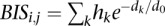 , where hk is the complex score of CRE k, dk is the distance between the TSS and the CRE. d0 is a constant used in the ratio dk /d0 to specify the shape of the exponential function (Ouyang et al. 2009); the larger d0, the more distal complexes will influence the promoter and eventually the BIS score. In this study, we set d0 to 5 kb, because using this value the corresponding regression models, used to integrate our binding data with gene expression, had the highest R2 (see next paragraphs). This parameter choice leads to a rapidly decreasing exponential function (Supplemental Fig. 12), which strongly penalizes distal regulatory elements, such as the “enhanceosome” complex (complex H-11 in Fig. 3A). To examine the effect of this parameter on the POU5F1–SOX2–NANOG complex, we changed d0 to higher values (i.e., 100 kb and 500 kb), in order to give higher BIS scores to complexes that bind to CREs far away from the TSS and repeated the regression analysis for the data shown in Figure 3A (H1 ESC data set, NMF run at k = 17). The new estimated regression coefficients for the POU5F1–SOX2–NANOG complex are now positive and statistically significant in both d0 = 100 kb and d0 = 500 kb (P < 0.003 and P < 2 × 10⁻¹⁶, respectively) (Supplemental Fig. 13). Thus, when allowing distal CREs to more strongly influence promoters, our analysis correctly predicts the positive transcriptional regulatory activity of POU5F1–SOX2–NANOG on its target genes.
The BIS values were then used as explanatory variables (predictors) to assess the contribution of a detected protein complex to gene expression (response). Linear regression was performed in R (function lm) using the model 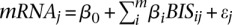 , where mRNAj is the absolute mRNA expression value of gene j, and BISij is the score of gene j in complex i. The
  coefficients were estimated using ordinary least square fitting and their statistical significance was determined using the t-test. A significant and positive
  coefficient indicates that the corresponding protein complex positively contributes to mRNA expression values, while a negative coefficient indicates negative (i.e., repressive) contribution.
Random forests regression (Breiman 2001) was also performed in R (package randomForest 4.6-4), a nonlinear regression technique that is based on an ensemble of trees, and the method of bootstrap aggregation (Breiman 2001). The performance of both models was evaluated by R2, which measures the quality of the overall fit of the model and indicates the proportion of the gene expression variation explained by the model, as well as by fourfold cross-validation, measuring goodness of fit, and prediction accuracy using Spearman correlation between actual and predicted gene expression values. The importance of the variables in random forests (function importance) is measured by the increased mean square error (Supplemental Fig. 9) that represents the deterioration of the predictive accuracy of the model when each component-predictor is replaced by random noise, as well as by the residual sum of squares that shows the decrease in node impurities from permutation of each predictor (Supplemental Fig. 15). The frequency of the variables used is another measure of importance (function varUsed) and shows how many times each predictor is used in the forest (Supplemental Fig. 15).
GeneMANIA physical interactions
We used the physical interaction networks available in the GeneMANIA (Warde-Farley et al. 2010) database (http://genemania.org/data/current/networks/Homo_sapiens.tgz) to find pairs of TFs within the predicted complexes that are known to physically interact. We only used the interaction data from physical interactions (e.g., iRefIndex, BioGRID) and not from co-expression, co-localization, or protein domain networks. Although redundant interactions may be included in the data set by sources with overlapping interaction data (e.g., BioGRID, IREF_GRID, IREF_OPHID, IREF_BIND), we count an interaction between a pair of proteins only once, even though it may be supported by multiple sources. Thus, the P-values shown in Table 1, Supplemental Table 3, and Supplemental Table 5 are not affected by the number of sources supporting a protein–protein interaction, but are calculated after estimating the number of physical interactions that occur overall in 10,000 sets of complexes with random sets of genes (of the same size with the corresponding complex). Columns 4 and 5 (GeneMANIA scores, Source of interaction) in Supplemental Tables 3 and 5 are only provided to further explain and support the interacting pair of proteins.
The validation of the complexes through known protein–protein interactions demands choosing a coefficients threshold in NMF that defines which TFs participate in a complex. If this cutoff is high (e.g., 0.7), only a few TFs are considered members of a complex (i.e., only the bright red colored TFs in each complex in Fig. 3A), while at lower cutoff (e.g., 0.1) more TFs are added in each complex. We chose this threshold to be 0.3 because the TFs with complex coefficients >0.3 represent on average the top 5% of the NMF coefficients matrices of Figure 3. Additionally, at higher cutoffs we get on average two to three TFs in each complex, thus overlooking larger complexes.
Finally, we repeated the protein–protein interactions analysis with the TF complex members shaped when coefficient >0.1 and found less significant protein–protein interactions within the complex members shaped at cutoff 0.1 than at 0.3.
Shuffling of the RC matrix
The ChIP-seq read densities were randomly shuffled within each CRE: The read density of a ChIP-seq experiment was randomly assigned to another experiment (Supplemental Fig. 10). NMF was subsequently performed on the shuffled RC matrix, and regression analysis followed using the BIS values of the new NMF-discovered complexes as explanatory variables, in order to assess the accuracy of both predictive regression models. The process of shuffling–NMF–regression was repeated 100 times, and the average R2 and correlation coefficients are shown in Figure 4. We observe that the predictive accuracy of the models is better without shuffling, suggesting that our method of inferring protein complexes with NMF based on the collective binding of multiple TFs on CREs can explain gene expression variation better than models that use random TF binding data.
Acknowledgments
We thank Renaud Gaujoux for assisting in certain aspects of the NMF analysis, Quaid Morris for his help with the GeneMANIA physical interactions data sets, and David S. Rickman and Yanwen Jiang for their insightful comments. This work was supported by the CAREER grant from the National Science Foundation (DB1054964), the Starr Cancer Consortium grant I4-A411, the LLS SCOR grant 7132-08, as well as by startup funds from the Institute for Computational Biomedicine, Weill Cornell Medical College.
Author contributions: E.G.G. developed the method, analyzed the results, and wrote the manuscript. O.E. supervised the project and edited the manuscript. Both authors read and approved the final manuscript.
Footnotes
[Supplemental material is available for this article.]
Article published online before print. Article, supplemental material, and publication date are at http://www.genome.org/cgi/doi/10.1101/gr.149419.112.
Freely available online through the Genome Research Open Access option.
References
- Barski A, Cuddapah S, Cui K, Roh TY, Schones DE, Wang Z, Wei G, Chepelev I, Zhao K 2007. High-resolution profiling of histone methylations in the human genome. Cell 129: 823–837 [DOI] [PubMed] [Google Scholar]
- Breiman L 2001. Random Forests. Mach Learn 45: 5–32 [Google Scholar]
- Brunet JP, Tamayo P, Golub TR, Mesirov JP 2004. Metagenes and molecular pattern discovery using matrix factorization. Proc Natl Acad Sci 101: 4164–4169 [DOI] [PMC free article] [PubMed] [Google Scholar]
- Cheng C, Gerstein M 2011. Modeling the relative relationship of transcription factor binding and histone modifications to gene expression levels in mouse embryonic stem cells. Nucleic Acids Res 40: 553–568 [DOI] [PMC free article] [PubMed] [Google Scholar]
- Cheng C, Alexander R, Min R, Leng J, Yip KY, Rozowsky J, Yan K-K, Dong X, Djebali S, Ruan Y, et al. 2012. Understanding transcriptional regulation by integrative analysis of transcription factor binding data. Genome Res 22: 1658–1667 [DOI] [PMC free article] [PubMed] [Google Scholar]
- Cuddapah S, Jothi R, Schones DE, Roh TY, Cui K, Zhao K 2009. Global analysis of the insulator binding protein CTCF in chromatin barrier regions reveals demarcation of active and repressive domains. Genome Res 19: 24–32 [DOI] [PMC free article] [PubMed] [Google Scholar]
- D'Apuzzo M, Mandolesi G, Reis G, Schuman EM 2001. Abundant GFP expression and LTP in hippocampal acute slices by in vivo injection of sindbis virus. J Neurophysiol 86: 1037–1042 [DOI] [PubMed] [Google Scholar]
- Elemento O, Slonim N, Tavazoie S 2007. A universal framework for regulatory element discovery across all genomes and data types. Mol Cell 28: 337–350 [DOI] [PMC free article] [PubMed] [Google Scholar]
- The ENCODE Project Consortium 2011. A user's guide to the Encyclopedia of DNA Elements (ENCODE). PLoS Biol 9: e1001046. [DOI] [PMC free article] [PubMed] [Google Scholar]
- The ENCODE Project Consortium 2012. An integrated encyclopedia of DNA elements in the human genome. Nature 489: 57–74 [DOI] [PMC free article] [PubMed] [Google Scholar]
- Ernst J, Kellis M 2012. ChromHMM: Automating chromatin-state discovery and characterization. Nat Methods 9: 215–216 [DOI] [PMC free article] [PubMed] [Google Scholar]
- Ernst J, Kheradpour P, Mikkelsen TS, Shoresh N, Ward LD, Epstein CB, Zhang X, Wang L, Issner R, Coyne M, et al. 2011. Mapping and analysis of chromatin state dynamics in nine human cell types. Nature 473: 43–49 [DOI] [PMC free article] [PubMed] [Google Scholar]
- Gaujoux R, Seoighe C 2010. A flexible R package for nonnegative matrix factorization. BMC Bioinformatics 11: 367. [DOI] [PMC free article] [PubMed] [Google Scholar]
- Gerstein MB, Kundaje A, Hariharan M, Landt SG, Yan K-K, Cheng C, Mu XJ, Khurana E, Rozowsky J, Alexander R, et al. 2012. Architecture of the human regulatory network derived from ENCODE data. Nature 489: 91–100 [DOI] [PMC free article] [PubMed] [Google Scholar]
- Giannopoulou EG, Elemento O 2011. An integrated ChIP-seq analysis platform with customizable workflows. BMC Bioinformatics 12: 277. [DOI] [PMC free article] [PubMed] [Google Scholar]
- Goke J, Jung M, Behrens S, Chavez L, O'Keeffe S, Timmermann B, Lehrach H, Adjaye J, Vingron M 2011. Combinatorial binding in human and mouse embryonic stem cells identifies conserved enhancers active in early embryonic development. PLoS Comput Biol 7: e1002304. [DOI] [PMC free article] [PubMed] [Google Scholar]
- Herrmann C, Van de Sande B, Potier D, Aerts S 2012. i-cisTarget: An integrative genomics method for the prediction of regulatory features and cis-regulatory modules. Nucleic Acids Res 40: e114. [DOI] [PMC free article] [PubMed] [Google Scholar]
- Hoffman MM, Buske OJ, Wang J, Weng Z, Bilmes JA, Noble WS 2012. Unsupervised pattern discovery in human chromatin structure through genomic segmentation. Nat Methods 9: 473–476 [DOI] [PMC free article] [PubMed] [Google Scholar]
- Johnson DS, Mortazavi A, Myers RM, Wold B 2007. Genome-wide mapping of in vivo protein-DNA interactions. Science 316: 1497–1502 [DOI] [PubMed] [Google Scholar]
- Karlic R, Chung HR, Lasserre J, Vlahovicek K, Vingron M 2010. Histone modification levels are predictive for gene expression. Proc Natl Acad Sci 107: 2926–2931 [DOI] [PMC free article] [PubMed] [Google Scholar]
- Kim H, Park H 2007. Sparse non-negative matrix factorizations via alternating non-negativity-constrained least squares for microarray data analysis. Bioinformatics 23: 1495–1502 [DOI] [PubMed] [Google Scholar]
- Kim J, Chu J, Shen X, Wang J, Orkin SH 2008. An extended transcriptional network for pluripotency of embryonic stem cells. Cell 132: 1049–1061 [DOI] [PMC free article] [PubMed] [Google Scholar]
- Lee BK, Bhinge AA, Battenhouse A, McDaniell RM, Liu Z, Song L, Ni Y, Birney E, Lieb JD, Furey TS, et al. 2012. Cell-type specific and combinatorial usage of diverse transcription factors revealed by genome-wide binding studies in multiple human cells. Genome Res 22: 9–24 [DOI] [PMC free article] [PubMed] [Google Scholar]
- Miele A, Dekker J 2009. Mapping cis- and trans-chromatin interaction networks using chromosome conformation capture (3C). Methods Mol Biol 464: 105–121 [DOI] [PMC free article] [PubMed] [Google Scholar]
- Moorman C, Sun LV, Wang J, de Wit E, Talhout W, Ward LD, Greil F, Lu XJ, White KP, Bussemaker HJ, et al. 2006. Hotspots of transcription factor colocalization in the genome of Drosophila melanogaster. Proc Natl Acad Sci 103: 12027–12032 [DOI] [PMC free article] [PubMed] [Google Scholar]
- Moqtaderi Z, Wang J, Raha D, White RJ, Snyder M, Weng Z, Struhl K 2010. Genomic binding profiles of functionally distinct RNA polymerase III transcription complexes in human cells. Nat Struct Mol Biol 17: 635–640 [DOI] [PMC free article] [PubMed] [Google Scholar]
- Nakamura T, Yamazaki Y, Saiki Y, Moriyama M, Largaespada DA, Jenkins NA, Copeland NG 2000. Evi9 encodes a novel zinc finger protein that physically interacts with BCL6, a known human B-cell proto-oncogene product. Mol Cell Biol 20: 3178–3186 [DOI] [PMC free article] [PubMed] [Google Scholar]
- Natarajan A, Yardımcı GG, Sheffield NC, Crawford GE, Ohler U 2012. Predicting cell-type–specific gene expression from regions of open chromatin. Genome Res 22: 1711–1722 [DOI] [PMC free article] [PubMed] [Google Scholar]
- O'Neil J, Look AT 2007. Mechanisms of transcription factor deregulation in lymphoid cell transformation. Oncogene 26: 6838–6849 [DOI] [PubMed] [Google Scholar]
- Ouyang Z, Zhou Q, Wong WH 2009. ChIP-Seq of transcription factors predicts absolute and differential gene expression in embryonic stem cells. Proc Natl Acad Sci 106: 21521–21526 [DOI] [PMC free article] [PubMed] [Google Scholar]
- Pascual-Montano A, Carazo JM, Kochi K, Lehmann D, Pascual-Marqui RD 2006. Nonsmooth nonnegative matrix factorization (nsNMF). IEEE Trans Pattern Anal Mach Intell 28: 403–415 [DOI] [PubMed] [Google Scholar]
- Pearson AG, Gray CW, Pearson JF, Greenwood JM, During MJ, Dragunow M 2003. ATF3 enhances c-Jun-mediated neurite sprouting. Brain Res Mol Brain Res 120: 38–45 [DOI] [PubMed] [Google Scholar]
- Pu Y, Tang GC, Wang WB, Savage HE, Schantz SP, Alfano RR 2011. Native fluorescence spectroscopic evaluation of chemotherapeutic effects on malignant cells using nonnegative matrix factorization analysis. Technol Cancer Res Treat 10: 113–120 [DOI] [PubMed] [Google Scholar]
- Rada-Iglesias A, Ameur A, Kapranov P, Enroth S, Komorowski J, Gingeras TR, Wadelius C 2008. Whole-genome maps of USF1 and USF2 binding and histone H3 acetylation reveal new aspects of promoter structure and candidate genes for common human disorders. Genome Res 18: 380–392 [DOI] [PMC free article] [PubMed] [Google Scholar]
- Rada-Iglesias A, Bajpai R, Swigut T, Brugmann SA, Flynn RA, Wysocka J 2011. A unique chromatin signature uncovers early developmental enhancers in humans. Nature 470: 279–283 [DOI] [PMC free article] [PubMed] [Google Scholar]
- Ram O, Goren A, Amit I, Shoresh N, Yosef N, Ernst J, Kellis M, Gymrek M, Issner R, Coyne M, et al. 2011. Combinatorial patterning of chromatin regulators uncovered by genome-wide location analysis in human cells. Cell 147: 1628–1639 [DOI] [PMC free article] [PubMed] [Google Scholar]
- Ravasi T, Suzuki H, Cannistraci CV, Katayama S, Bajic VB, Tan K, Akalin A, Schmeier S, Kanamori-Katayama M, Bertin N, et al. 2010. An atlas of combinatorial transcriptional regulation in mouse and man. Cell 140: 744–752 [DOI] [PMC free article] [PubMed] [Google Scholar]
- Rickman DS, Soong TD, Moss B, Mosquera JM, Dlabal J, Terry S, MacDonald TY, Tripodi J, Bunting K, Najfeld V, et al. 2012. Oncogene-mediated alterations in chromatin conformation. Proc Natl Acad Sci 109: 9083–9088 [DOI] [PMC free article] [PubMed] [Google Scholar]
- Roder K, Wolf SS, Larkin KJ, Schweizer M 1999. Interaction between the two ubiquitously expressed transcription factors NF-Y and Sp1. Gene 234: 61–69 [DOI] [PubMed] [Google Scholar]
- Rye M, Saetrom P, Handstad T, Drablos F 2011. Clustered ChIP-Seq-defined transcription factor binding sites and histone modifications map distinct classes of regulatory elements. BMC Biol 9: 80. [DOI] [PMC free article] [PubMed] [Google Scholar]
- Shen Y, Yue F, McCleary DF, Ye Z, Edsall L, Kuan S, Wagner U, Dixon J, Lee L, Lobanenkov VV, et al. 2012. A map of the cis-regulatory sequences in the mouse genome. Nature 488: 116–120 [DOI] [PMC free article] [PubMed] [Google Scholar]
- Tabach Y, Brosh R, Buganim Y, Reiner A, Zuk O, Yitzhaky A, Koudritsky M, Rotter V, Domany E 2007. Wide-scale analysis of human functional transcription factor binding reveals a strong bias towards the transcription start site. PLoS ONE 2: e807. [DOI] [PMC free article] [PubMed] [Google Scholar]
- van der Vlag J, Otte AP 1999. Transcriptional repression mediated by the human polycomb-group protein EED involves histone deacetylation. Nat Genet 23: 474–478 [DOI] [PubMed] [Google Scholar]
- Visel A, Blow MJ, Li Z, Zhang T, Akiyama JA, Holt A, Plajzer-Frick I, Shoukry M, Wright C, Chen F, et al. 2009. ChIP-seq accurately predicts tissue-specific activity of enhancers. Nature 457: 854–858 [DOI] [PMC free article] [PubMed] [Google Scholar]
- Wang C, Tian R, Zhao Q, Xu H, Meyer CA, Li C, Zhang Y, Liu XS 2012a. Computational inference of mRNA stability from histone modification and transcriptome profiles. Nucleic Acids Res 40: 6414–6423 [DOI] [PMC free article] [PubMed] [Google Scholar]
- Wang J, Zhuang J, Iyer S, Lin X, Whitfield TW, Greven MC, Pierce BG, Dong X, Kundaje A, Cheng Y, et al. 2012b. Sequence features and chromatin structure around the genomic regions bound by 119 human transcription factors. Genome Res 22: 1798–1812 [DOI] [PMC free article] [PubMed] [Google Scholar]
- Warde-Farley D, Donaldson SL, Comes O, Zuberi K, Badrawi R, Chao P, Franz M, Grouios C, Kazi F, Lopes CT et al. 2010. The GeneMANIA prediction server: Biological network integration for gene prioritization and predicting gene function. Nucleic Acids Res 38: W214–W220 [DOI] [PMC free article] [PubMed] [Google Scholar]
- Xu M, Li W, James GM, Mehan MR, Zhou XJ 2009. Automated multidimensional phenotypic profiling using large public microarray repositories. Proc Natl Acad Sci 106: 12323–12328 [DOI] [PMC free article] [PubMed] [Google Scholar]
- Yu HB, Johnson R, Kunarso G, Stanton LW 2011. Coassembly of REST and its cofactors at sites of gene repression in embryonic stem cells. Genome Res 21: 1284–1293 [DOI] [PMC free article] [PubMed] [Google Scholar]
- Zhang J, Kalkum M, Yamamura S, Chait BT, Roeder RG 2004. E protein silencing by the leukemogenic AML1-ETO fusion protein. Science 305: 1286–1289 [DOI] [PubMed] [Google Scholar]