

Abstract
Electron transfer (ET) reactions are one of the most important processes in chemistry and biology. Because of the quantum nature of the processes and the complicated roles of the solvent, theoretical study of ET processes is challenging. To simulate ET processes at the electronic level, we have developed an efficient DFT QM/MM approach that uses the fractional number of electrons as the order parameter to calculate the redox free energy of ET reactions in solution. We applied this method to study the ET reactions of the aqueous metal complexes and . The calculated oxidation potentials, 5.82 eV for Fe(II/III) and 5.14 eV for Ru(II/III), agree well with the experimental data, 5.50 eV and 4.96 eV, for iron and ruthenium, respectively. Furthermore, we have constructed the diabatic free energy surfaces from histogram analysis based on the molecular dynamics trajectories. The resulting reorganization energy and the diabatic activation energy also show good agreement with experimental data. Our calculations show that using the fractional number of electrons (FNE) as the order parameter in the thermodynamic integration process leads to efficient sampling and validate the ab initio QM/MM approach in the calculation of redox free energies.
I. INTRODUCTION
As one of the fundamental processes in biology and chemistry, electron transfer (ET) reactions have been the focus of experimental and theoretical studies for decades.1 The most widely used theory for electron transfer was developed by Marcus in the 1950s based on a simplified description of the solvent behavior, specifically a continuum solvent model with the linear response assumption.2–5 Marcus theory has been applied extensively to molecular systems and can yield qualitatively correct results for molecules with drastically different chemical compositions. However, because of the simplified solvent models, Marcus theory does not provide the details of the solvent dynamics and the effects of solute inner structure in ET processes, and thus may lead to deviation in complex cases.1,6 To understand the detailed kinetics, thermodynamics, and mechanism of ET processes, simulation study at the atomistic and electronic level becomes necessary.
Consistent with the framework of Marcus theory, a straightforward approach for calculating the redox potentials is to compute the energetic change of ET processes with a quantum mechanical (QM) treatment of the solute and an implicit model for the contributions of the solvent molecules, e.g., the dielectric continuum model. It is often thought that such a computational scheme can capture the most important quantum mechanical nature of ET processes with a reasonable description of the solvent effects.7–9 The advantage of this approach is clearly the reduced computational cost for the solvent molecules, such that highly accurate DFT and even MP2 calculations are now affordable for the energetic calculation of the redox center. However, the QM optimized geometry of the reaction site has a crucial influence on the final energetics. The calculated redox potentials and inner shell reorganization energy can depend on the solute geometry and the size of the QM region, as found in a recent study7 where the solute molecules in the presence of the continuum solvent have been carefully examined with DFT calculations. Furthermore, the fluctuations of the solvent molecules, which constitute the driving force for ET processes, are also absent in this simplified theoretical scheme. Such an effect can only be obtained with explicit treatment of the solvent molecules in ensemble-based phase space sampling simulations.
Because of the limitation of computer resources, early efforts to incorporate the explicit contribution of the solvent molecules through broad phase space sampling were realized with a simplified molecular mechanical (MM) description of the reaction system. In the 1980s, Warshel et al.10–13 and Kuharski et al.14 performed a series of simulations of ET processes with MM force fields. These calculations showed that with the classical solvent model and a specially designed MM force field for the solute, the essential solvent behavior and contributions can be correctly simulated. Nonetheless, since the MM force fields used cannot describe the electronic structures of the ET reaction centers, the calculated redox potentials may not be directly comparable to experimental values.15
Recent advances in computational resources have enabled simulations of ET processes with ab initio molecular dynamics (MD) methods, such as the Car-Parrinello molecular dynamics (CPMD) method.16 Sprik’s group has successfully employed the CPMD method to simulate ET in several aqueous metal complexes.17–22 In these studies, the whole system including the solvent molecules was treated quantum mechanically and the time evolution of the electronic structures was modeled with CPMD based on a plane-wave implementation of density functional theory (DFT). Compared with simple MM force fields, treating the whole system quantum mechanically, including both the solute and the solvent molecules, certainly improves the accuracy of the results. However, the computational cost is demanding such that the calculation can only be performed on a system of limited size on a short timescale, which may lead to convergence issues in the final results.19
The combined quantum mechanics and molecular mechanics (QM/MM) method, initially developed by Warshel and Levitt,23 enables a good balance between computational accuracy and efficiency and has become a promising alternative for studying chemical reaction processes, including ET reactions. By describing the solute with highly accurate QM methods and the solvent molecules with classic MM methods, QM/MM calculations can provide satisfactorily accurate energetics at reasonable computational costs.24,25 Applications of QM/MM methods to the calculation of redox potentials have been reported, but more often with some level of approximations to reduce the amount of calculations. Either the QM calculations are avoided in the MD sampling and replaced by geometry optimization or a frozen DFT approach,26 or semi-empirical QM methods are employed in MD simulations.27 A few examples have been reported in which ab initio QM/MM methods are applied together with MD sampling.28,29
To improve the accuracy of the calculations and the convergence of the free energy simulation of ET processes, we have developed here a first-principle QM/MM-MD method to simulate ET processes using the fractional number of electrons as an order parameter. The use of the fractional number of electrons yields additional efficiency in free energy simulations as compared with other simulation methods. The explicit treatment of solvent molecules does not assume the linear response of the solvent. In addition, QM/MM methods are applicable to complex systems such as proteins and enzymes.
This paper is organized as follows. We first review the background on Marcus theory, ET half-reactions, and free energy simulation methods. Then we introduce the fractional electron approach. In Sec. III we show the computational details of our simulations. In Sec. IV we reconstruct the diabatic free energy surfaces from the simulation trajectory with histogram analysis12 and compare the simulation results with other theoretical work and experiments. Finally we conclude with Sec. V.
II. THEORY
A. Background
1. Marcus Theory
In Marcus theory, the solvent and solute contribution in the ET process is described as the reorganization energy λ, which is defined to be the decrease on the free energy surface along the reaction coordinate ξ (see Fig. 1),
Figure 1.

Diabatic free energy surfaces in electron transfer process. The free energy curves of reactant and product states were plotted with respect to the reaction coordinate ξ. ξr,p denote the expectation values of the reaction coordinate of the reactant and product, respectively. ΔG is the thermodynamic free energy, ΔG‡ is the diabatic activation free energy, and λr;p are the solvent reorganization energies for the reactant and product, respectively.
| (1) |
| (2) |
where, λr,p, Gr,p and ξr,p are reorganization energies, free energies, and the reaction coordinate for the reactant and product states, respectively.
The reorganization energy can be divided into the outer shell solvent contribution and the inner shell solute contribution. Based on the linear response approximation assumed in the dielectric continuum solvent model, the outer shell solvent reorganization energy is derived to be a function of the transferred charge Δq, the solvent dielectric properties εe and εs, the radii rA,B of the solutes and the separation RAB of electronic centers (A and B),
| (3) |
The linear response assumption of the solvent led to the famous Marcus parabolas (Fig. 1) for the diabatic energy surfaces along the reaction coordinate for both reduced and oxidized states. According to Marcus theory, the outer shell activation free energy , the barrier at the intersecting point of the two free energy curves, is related to the thermodynamic driving force and the solvent reorganization energy,
| (4) |
For self-exchange reaction, the thermodynamic free energy ΔG is equal to 0, which allows Eq. (4) to be simplified as . In the original model, the inner shell reorganization energy was not considered because the solute was treated as a spherical body, but the intramolecular contribution to the activation free energy was thereafter studied and included.30
2. ET Half-Reactions
For convenience, aqueous self-exchange reactions of metal complexes (Eq. (5)) are often chosen as the simplest model to study solvated ET reactions.
| (5) |
e.g., M = Fe, Ru.
The attempt to calculate the full reaction with DFT calculation is very challenging because ET reactions are a type of special electronic excitation problem. Although a recent work using spin-polarized DFT31 shows encouraging result for the full ET reaction, this problem can often be avoided by dividing the full reaction into two half-reactions, assuming the reaction is carried out via an electron reservoir as the mediator.19 The half-reaction in the simulation is
| (6) |
3. Free Energy Simulation
In the studies of ET reactions, the redox free energy ΔG and activation energy ΔG‡ are of great importance because they determine the reaction equilibrium constant and rate constant, respectively. Like many other chemical reactions, the free energy for a half-reaction can be computed with various free energy simulation methods. Free energy perturbation (FEP),32 thermodynamic integration (TI),33 and umbrella sampling34 are commonly employed methods in free energy simulations. In the TI method, ΔA is evaluated as an integral over the derivative of the potential energy with respect to an order parameter (η) in the ensemble average.
| (7) |
where A is the Helmholtz free energy, and 〈···〉η denotes the ensemble average of the biased sampling window at order parameter η, which is defined between the reactant state (η = 0) and the product state (η = 1). For ET reactions that occur under constant temperature and pressure, the Gibbs free energy ΔG can be approximated by the Helmholtz free energy ΔA.
B. Fractional Number of Electrons as the Order Parameter
Unlike chemical reactions, which can often be well characterized by the geometrical change of a set of atoms, electron transfer may not proceed in parallel with the geometrical changes at the reaction site. To apply the TI method to simulate the free energy change, the immediate question is to identify a suitable order parameter that distinguishes the reactant and product states,35 and can drive the system from one state to the other to enable the sampling of the free energy surface. One common choice is to use a coupling parameter to mix the potential energy surfaces of two states.33 In this fashion, the effective energy and forces are calculated through linear coupling of two calculations: one for the reduced state and the other for the oxidized state.
Instead of mixing two energy functions to describe the transition, an alternative approach is to gradually change the number of electrons in the system.14 MD sampling can be performed with the QM energy and forces computed by fixing the FNE of the system in the SCF calculations. Thus for each conformational state, only one QM calculation at the specific FNE state is required to generate the energy and forces. Compared with the coupling parameter method, the FNE approach requires only half the computational cost. This advantage has indeed been taken in previous work.31,36,37
When the FNE is employed as the order parameter (η), the oxidation process can be represented as in Fig. 2. The corresponding state of the system with FNE is,
Figure 2.
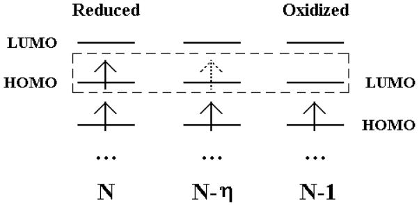
Scheme of oxidation process. The arrows denote electrons and the horizontal bars are orbitals. In oxidation process, we remove the FNE on the HOMO of the reduced state with N electrons, and gradually reaches the oxidized state with (N − 1) electrons.
| (8) |
The physical significance of the fractional electron can be interpreted as the probability of the electronic distribution on the HOMO of the solute.38,39 For example, the state corresponds to the ensemble with half of the systems in the reduced state (i.e. ) and half of the systems in the oxidized state (i.e. ).
Known36,37,40,41 as the Janak theorem, the energy derivative with respect to the occupation number in the highest occupied Kohn-Sham orbital in DFT calculation is equal to its orbital energy εHOMO. Cohen, Mori-Sanchez and Yang have recently proved that this indeed is also the derivative of the total DFT energy with respect to the total number of electrons for DFT calculations with exchange-correlation functionals being explicit functional of density (such as the local density approximation).42,43 Thus, we have
| (9) |
where the minus sign is introduced because η is the fractional number of electrons removed from the HOMO, and the occupation number of the orbital is actually (1 − η). Thus, the redox free energy can be then conveniently evaluated from thermodynamic integration of the HOMO energies, i.e.
| (10) |
When the DFT calculations are performed with orbital functionals beyond the local density and generalized gradient approximations, the corresponding derivative of the total DFT energy with respect to the total number of electrons has also been derived.42,43
C. Reaction Coordinate and Free Energy Surface
When the QM/MM-MD simulation is completed, the values of 〈εHOMO〉η are available, and the redox free energy can be easily obtained with the TI method. In most cases, the reorganization and activation free energy of the reaction can also be obtained. A reaction coordinate must be defined to reconstruct the diabatic free energy surface similar to the scheme in Fig. 1. The order parameter η cannot serve this role because the FNE is only an electronic coordinate for the ET reaction, which was introduced to perform effective sampling but contains no information of the solvent dynamics. Instead, a reaction coordinate containing solvent statistics is required at this stage to characterize the dynamics and mechanism of the reaction.21,35 The energy gap between the reactant and product states at the same nuclear configuration10 often serves as a convenient reaction coordinate to characterize the solvent contribution in the reaction,
| (11) |
where E0(R) and E1(R) are the potential energies of the reactant and product, at the solute and solvent nuclear configuration R. In order to use the energy gap as the reaction coordinate, dual calculations (for the reduced and oxidized states) must be performed for each configuration. But these calculations are only needed for the data points necessary for histogram analysis, which is normally less than one tenth of the total MD sampling points. Hence the calculation for the energy gap will not significantly increase the overall computational cost. With the reaction coordinate, the histogram analysis12 can be performed to obtain the probability distribution and to reconstruct the diabatic free energy surfaces of the systems.
The redox half-reactions in Eq. (6) can be interpreted as the electron transfer from the solute in the reduced state to an ideal electrode with electronic chemical potential μ. Therefore, the potential energy of the reactant state corresponds to that of the reduced state, i.e. E0 = ERe, while the potential energy of the product state E1 contains the potential energy of both the oxidized solute and the electrode, i.e., E1 = EOx + μ. Thus, the representation of energy gap in the half-reaction simulation is,
| (12) |
From the histogram analysis of the dynamics trajectories, the probability distribution of the energy gap P0,1(ΔE) can be obtained as,
| (13) |
The corresponding potential of mean force along the reaction coordinate ΔE in the diabatic representation for the reactant state 0 (reduced state) and product state 1 (oxidized state with the electron transferred to the ideal electrode) are,
| (14) |
| (15) |
where ∫dR denotes integration over both the solute and solvent coordinates, β = 1/kBT is the inverse of the product of Boltzmann constant and temperature, A0,1 = −kBT ln ∫dRe−βE0,1(R) is the free energy of the reactant or the product state, and P0,1 is the probability distribution of the reaction coordinate.
D. Reorganization Energies
Once the diabatic free energy surfaces has been obtained, we can measure the reorganization energies of the half-reactions according to the definition in Eqs. (1–2), i.e.,
| (16) |
| (17) |
where ΔE0,1 is the ensemble average of the energy gap in state 0, 1. Since the reorganization energy is the free energy decrease on the same diabatic surface, thus this quantity is independent of μ, meaning the chemical potential can be chosen arbitrarily. For convenience, μ is chosen to be the negative oxidation free energy, i.e., μ = −ΔA = ARe − AOx, so that the free energy difference between the reactant and product states becomes zero, and the diabatic free energy surface of the oxidized state is shifted to be: A1(ΔE) = AOx(ΔE) + μ. Because the free energy surface is only shifted for a constant μ, the reorganization energy remains unchanged, i.e., λRe = λ0 and λOx = λ1.
In our QM/MM approach, the quantities so obtained include both the inner shell reorganization energy λin from the solute geometry change and the outer shell reorganization energy λout from the solvent contribution. Thus, they should be interpreted as the total reorganization energies of the half-reactions, .
To help understanding the ET processes, we decomposed the calculated total reorganization energies into the inner and outer shell contributions. Usually, the inner shell reorganization energies can be calculated from the bond length changes and the bond force constants with the harmonic model for molecular vibration.7,44–46 The inner shell reorganization energies can also be obtained from direct MD simulations in vacuo15 with the assumption that the bulk solvent has negligible influence on the inner shell reorganization process. Although the inner shell reorganization energy only contains the contributions from the solute, the presence of solvent may affect the vibrational motions of solute molecule. In some cases, the inner shell reorganization energy from MD simulation in vacuo was reported to be even larger than the total reorganization energy,15 which indicates that the effect of solvent on inner shell may be important.
In our approach, the inner shell reorganization energies of the half-reactions can be directly obtained without the above assumptions. We can obtain free energy contributions of the solute explicitly from the trajectories of the solute molecules in the MD simulation. By replaying the trajectories of the solute molecules without the surrounding MM solvent, we can exclude the solvent contributions while including the solvent influence on inner shell motions, since the snapshots are taken from the MD simulation in solution. Histogram analysis can then be performed on the solute trajectories in order to obtain the diabatic free energy surfaces only for the solute molecules,
| (18) |
where r is only the solute coordinates, is the free energy of the solute, is the potential energy of the solute, and ΔE′ is the energy gap between two redox states of the solute molecule. Based on the free energy surfaces only for the solute, the inner shell reorganization energies can be measured according to the definition,
| (19) |
| (20) |
where the solute free energy surfaces can also be shifted to the same baseline without affecting the value of the inner shell reorganization energies.
III. COMPUTATIONAL DETAILS
Hexaaquo ruthenium and iron cations, and , were selected as the two test systems to evaluate the performance of our approach. The geometrical changes of the two coordination compounds and during the redox process are not significant. Only slight changes (~0.1 Å) in the coordination bond lengths were observed experimentally44,47 and in our calculations. Since the dielectric continuum model is a good approximation for aqueous solution, these two systems comply well with Marcus theory. For this reason the two systems have been studied extensively by both experimental and theoretical work.
The QM regions in both systems were defined as the central metal cation with six coordinating water molecules, i.e. , and . The initial geometries of the complexes were optimized in the gas phase. The QM subsystems of and were further solvated by 8641 and 8638 MM water molecules respectively, treated with the TIP3P model.48 The entire system for each simulation was in a cubic box with side length 64 Å under periodic boundary conditions.
The MD simulations were carried out with the Sigma49,50 program combined with Gaussian0351 for the QM calculations.52 Spin-unrestricted DFT calculations were performed for the QM subsystem, with the BLYP exchange-correlation functional.53,54 The effective core potential (ECP) basis set LanL2DZ55 was used for both the metal ion and the ligand molecules. The DFT calculation with FNE was carried out with a modified version of the Gaussian03 program, which uses a fraction occupation number of the HOMO during the SCF calculation. One SCF calculation was performed at each MD step to evaluate the energy and forces on the QM system. The parameters of the CHARMM force field56 and parameters from Ref.57 for Ru were used to model the classical MM interactions. The interactions between the QM and MM subsystems were described by van der Waals interactions and the electrostatic forces between point charges on MM water molecules based on the TIP3P model and the effective charges on QM atoms obtained from electrostatic potential (ESP) fitting.58,59 Because the long range electrostatic interaction between the solvent and the solute is essential for stabilizing the net charge on the system, and the Ewald summation for charged systems with a local basis set has not been implemented, a QM-MM interacting distance cutoff was used in our calculations and its influence on energetic properties was examined.
The QM/MM-MD simulations of were carried out for 18 ps after equilibration for 5 ps. The MD integration time step was 1 fs. Six windows with different values of fractional number of electrons, η = 0.0, 0.2, 0.4, 0.6, 0.8, 1.0, were used in the thermodynamic integration simulation from to . Similar simulations of were performed for 12.6 ps after 5 ps equilibration for each sampling window. The snapshots from trajectories were recorded every 9 fs, which provided 2000 and 1400 conformations from each sampling window of the Ru and Fe systems, respectively, for histogram analysis.
IV. RESULTS AND DISCUSSIONS
A. Oxidation Free Energy of Half-Reactions
The experimental oxidation free energy ΔG can be obtained from the electrode potential of the half-reaction φ from the Nernst equation (ΔG = −nFφ). For comparing experimental values with the simulation results, the absolute potential of the standard hydrogen electrode (SHE) should be added to the experimental electrode potentials. By taking −4.73 V for the absolute potential of the Pt-H electrode suggested by Reiss et al.60, the absolute oxidation free energies are 5.50 eV and 4.96 eV for aqueous and couples, respectively.
The oxidation free energies of aqueous and were obtained using the FNE-adapted thermodynamic integration, according to Eq. (10). The εHOMO curves along different fractional number of electrons η for the and systems are shown in Fig. 3. By integrating over the εHOMO curves, we obtained 5.14 eV and 5.82 eV for the absolute free energies ΔGAbs of and , respectively, which show good agreement with the experiment values (see Table I). From the difference between the absolute values of the two redox species, the relative free energy difference ΔΔG was found out to be 0.68 eV. This value can be compared to the experimental value 0.54 eV, which is directly obtained from the electrode potentials 0.77 V and 0.23 V of the aqueous iron and ruthenium ions, respectively, independent of the absolute value of the hydrogen electrode potential. Thus the ΔΔG error is 0.14 eV, which is smaller than the error in the absolute free energies (0.18 eV and 0.32 eV) and reflects the intrinsic accuracy of our method.
Figure 3.

Ensemble average of εHOMO curves for the two test systems at different fractional numbers of electrons. Their oxidation free energies are annotated, respectively, according to Eq. (10). The vertical bars indicate thermodynamic fluctuations.
Table I.
Comparison of the oxidation free energies of the aqueous and calculated with different methods and statistical approaches to experiments. Energy units are in eV.
B. Reorganization Free Energies of Half-Reactions
The probability distributions shown in Fig. 4A for the two systems along the energy gap ΔE from different sampling windows have sufficient overlap to enable the use of histogram analysis and the reconstruction of the diabatic free energy surfaces of the initial and final states as shown in Fig. 4B. The reorganization energies for each system were then obtained according to Eqs. (16–17). The total reorganization energy of the oxidized state λOx is 2.47 eV for the aqueous Fe complex and 2.52 eV for the Ru complex, which are comparable to corresponding experimental values listed in Table II.
Figure 4.

Energetic profile of the half redox reactions for and in aqueous solution. (A) Probability distributions over the order parameter ΔE for different sampling windows, and (B) energy surfaces of the initial and final states constructed from the probability distributions.
Table II.
Comparison of the reorganization energies and activation free energies of aqueous and calculated with different methods to experiments. Energies are in eV.
| Reorganization energies (half-reaction)§ | Activation Energies (full reaction) | ||||||||||||||
|---|---|---|---|---|---|---|---|---|---|---|---|---|---|---|---|
| λRe | λOx | λOx |
|
|
|
ΔG‡ | |||||||||
| QM/MMa | CPMDb | MMb | Expt. | QM/MMa | Expt.e | QM/MMf | CPMD | MM | Expt. | ||||||
|
|
2.41 | 2.52 | - | - | 2.11c | 0.35 | 0.41 | 0.60 | 1.22g | 0.79h | 0.49i | 0.9j | 0.69k | ||
|
|
2.43 | 2.47 | 0.78 | 0.42 | 1.54d | 0.37 | 0.34 | 0.34 | 1.28g | 0.80h | 0.20b | 0.08b | 0.51l | ||
Including both inner shell and outer shell reorganization energy for the oxidized state.
Results from this work.
Ref.15
Directly measured in photoelectron emission experiments.61
Calculated from the bond length differences and force constants.44,63,64,69 Experimental values of inner shell reorganization energies are the same for different redox states, since the force constants were assumed to be the same.
Results from this work.
Estimated in the infinite-separation limit.
Estimated in the touching-sphere limit.
Ref.31
Ref.14
Ref.47
Ref.44
The experimental reorganization energy for the oxidized Fe complex 2.11 eV was directly measured by photoelectron emission for the half-reaction61. However, similar experimental data for Ru is not available, thus the experimental value for the oxidized Ru complex was estimated by combining the experimental outer and inner shell reorganization energies,62–64 which is about 1.54 eV.
Comparing the calculation results with the experimental values, we found an overestimation in the total reorganization energies in the calculations, which may be due to the non-polarizable solvent model employed in our simulations. However, the better agreement between the calculation results and experimental values in the Fe complex than in the Ru complex suggests that the direct measurement of reorganization energy in photoelectron experiments (in the case of Fe) may be more accurate than combining the experimental outer and inner shell reorganization energies (in the case of Ru).
From the results demonstrated in Fig. 5, the inner shell reorganization energies of the half-reactions were found to be 0.35 eV and 0.41 eV for the oxidized and reduced Ru complex, and 0.37 eV and 0.34 eV for the oxidized and reduced Fe complex. These results are comparable to the experimental estimation of the inner shell reorganization energies, 0.60 eV for Fe and 0.34 eV for Ru,44,64 as shown in Table II. The experimental inner shell reorganization energy of each solute was obtained from the X-ray measurement of the coordination bond length changes,44,64 thus the inner shell reorganization energies for the two redox states are approximately the same, i.e., , based on a conventional assumption that the solute in different redox states has the same force constants of the coordination bond.
Figure 5.

Intramolecular diabatic free energy surfaces of the complex molecules (A) and (B) constructed from the probability distributions.
The results from the QM/MM simulation indicate that the solute intramolecular degrees of freedom have considerable contributions to the total reorganization free energies during the ET process, which agrees well with experiments.44,64 The better agreement in the inner shell than in the outer shell reorganization energies indicates that the QM calculations of the solute are quite accurate, which supports the speculation that the non-polarizable model for the MM solvent is an important error source in the reorganization energy calculation.
Based on the diabatic free energy surfaces in Fig. 4B and Fig. 5, for both systems, the total and inner shell reorganization energies are not the same for the reduced and oxidized states. The reorganization energies of the different redox states characterize different relaxation processes: λRe is the free energy decrease of the system after a vertical reduction, whereas λOx is the free energy decrease after a vertical oxidation. The observed free energy differences of about 0.1 eV imply the intrinsic difference of the solvent contributions to the two redox states, e.g., the force constants of the coordination bonds are not the same for the two different redox states.
C. Activation Free Energies
The quadratic shape of the diabatic free energy surfaces obtained from the non-Boltzmann sampling indicates that the FNE is an efficient order parameter. When the system reaches the intersection on the energy surface shown in the Fig. 4, the reaction coordinate ΔE is equal to zero, which means the electron can transfer from the solute to the reservoir with energy being conserved. At this point, the system evolves from the reactant state to the product state, which corresponds to the transition states in the Marcus perspective. Thus we can estimate the activation free energy for the half-reaction ,15 as the barrier height from the equilibrated reactant state to the transition state. However, the activation energy for the full self-exchange reaction is dependant on the separation distance between the two redox centers. In our work, since the two redox centers were treated separately as two half-reactions, we cannot identify the separation distance between two reacting redox solutes. Therefore, we examine the system in two extreme conditions and calculated the activation free energies in both cases, as summarized in Table II.
Infinite-separation limit
By assuming that the donor and acceptor are separated by a infinite distance, we can approximate the activation free energies of the full self-exchange reaction as , Under this assumption, the activation free energies for the full self-exchange reactions of the two complexes are 1.22 eV and 1.28 eV for Fe and Ru, respectively. In the infinite-separation limit, the solute molecules in the ET reaction are connected with an fictitious electron reservoir, and the distance between the two redox centers are assumed to be infinite, whereas in the experimental condition, the solutes are separated by a finite distance with the similar magnitude of the sum of their ionic radii. This difference leads to an overestimation in the free energy of the full reaction, despite of the accuracy in the half-reaction calculation. The experimental values of the activation energy are measured to be 0.69 eV and 0.51 eV for Fe and Ru, respectively.44,47 When compared to experimental values, the activation energies in our calculation at the infinite-separation limit are overestimated by 0.5~0.7 eV.
Touching-sphere limit
Unlike the redox free energy, which is independent of the path, the activation energy is dependent on the solvent conformation at the transition states. Compared to the more accurate results for the redox free energies, the observed larger deviations in the activation energy can be attributed to several factors. As described above, the difference between the infinite-separation limit and the real experimental condition actually contributes a significant proportion to the error, because we know from Marcus theory (Eqs. (3–4)) that the activation free energy depends on the distance between the two redox centers. In the experiment condition, the real distance cannot to be too large otherwise the electron tunneling probability will be too low. Thus, we here assumed the lower limit of the separation distance and use Marcus theory to correct the calculation results.
Based on the assumption that the solute radii are approximately the same for both redox states, and taking a limit that the distance between the two redox centers are equal to the sum of the radius of each solute, i.e., R = rOx + rRe ≈ 2rOx/Re, the outer shell reorganization energy for the full reaction is approximately equal to that for a half-reaction according to Eq. (3),62
| (21) |
where the notation follows that in Eq. (3). However, the inner shell reorganization energy for the full reaction maintains the additive relation,
| (22) |
Therefore, in this “touching-sphere” limit, the total reorganization energy for the full reaction is,
| (23) |
From the harmonic vibration model and the diabatic free energy surfaces of solute molecules in Fig. 5, we can assume that the Marcus relation is also applicable to the inner shell part in these two self-exchange reactions, i.e., . In the touching-sphere limit, the total activation energy can be estimated from the reorganization energy according to Marcus theory,
| (24) |
| (25) |
| (26) |
Feeding in the reorganization energies, the activation free energies for the self-exchange reactions of and are 0.79 eV and 0.80 eV, respectively, in much better agreement with experimental values. The activation free energies reduced by 0.4 ~ 0.5 eV in taking the touching-sphere limit compared to the infinite-separation limit.
The significant different results obtained in the infinite-separation limit and in the touching-sphere limit indicate that the relative geometrical conformation of the redox centers is important for obtaining the accurate activation energy of an ET reaction. In principle, the possible separation distance should be in between the two extremes; however, the real experimental condition is more similar to the touching-sphere limit.14,65,67 Although taking the touching-sphere limit reduced the error and generate more accurate activation energies for the two systems, we should be careful to apply this correction to other systems, where the assumption on the similarity of the radii of the two redox centers may be invalid. Despite the effect of the separation distance between the solutes, other factors may also introduce errors in the calculation of activation free energy. The non-polarizable water model may not be sufficient to simulate accurately the solvent conformation for the transition state. Additionally, the nuclear tunneling effects can also be important for obtaining accurate activation free energies in the process, which are not included in our work. For the aqueous iron complex, the nuclear tunneling probability, calculated from the overlap of the wave-functions of two nuclear configurations, enhances the self-exchange rate by a factor of about 60, equivalent to reducing the activation energy by 0.1 eV.66 Because a smaller geometric difference of the inner shell was observed in the redox process of than that of ,64 the nuclear tunneling factor may be even larger in the aqueous ruthenium. Each issue described above can introduce an error in the estimated activation energy.
D. Effect of the Long Range QM-MM Interaction Cutoff
As mentioned in Sec. III, QM-MM interaction distance cutoff was used in the simulation. Now we examine the influence of cutoff on the solute in terms of potential and HOMO energies. Unlike in the simulation of the full reaction, in which the net charge remains constant, the electrostatic environment of the half-reaction changes more dramatically during the electron transfer process because of the variation in the net charge of the system. Therefore, a commonly used interaction cutoff (~10 Å14,67 ) was found to be insufficient in the half-reaction simulation. By investigating the electrostatic potentials generated by solvent molecules at the center of the solute (see Fig. 6), we found that the solvent electrostatic potential do not converge until the cutoff distance reaches ~25 Å.
Figure 6.

The external electrostatic potentials generated by solvent molecules at the center of the periodic box for reduced and oxidized metal cations, respectively. The two solid lines correspond to ruthenium system and the dashed lines denote the iron system. The QM system is located at the center of the box, where the external potentials are plotted. The external potentials converge to constants as the QM-MM interaction cutoff increases.
Since the HOMO energies include the contributions from the QM-MM interactions, they consequently display similar slow convergence with respect to the interaction cutoff distance. As shown in Fig. 7, the HOMO energies are shifted by the external potential of the solvent molecules as far as 20 Å away from the central ion. The large interacting distance may be caused by the non-polarizable water model used since the polarization of the solvent could have screening effects and thus reduce the influence of the electrostatic interactions. Therefore, a periodic box with 64 Å for the side length was used and a radial cutoff of 28 Å for the QM-MM interactions was chosen in the MD simulations to ensure that the orientation of the solvent molecules was isotropic and the contributions from external electrostatic potential are converged.
Figure 7.

Dependence of the average of εHOMO curves for aqueous iron (A1) and ruthenium (B1) systems on the cutoff of QM-MM interaction distance. In (A2) and (B2), the difference of the εHOMO between the oxidized and reduced states (ΔεHOMO = εHOMO (Ru3+) −εHOMO (Ru2+)) are plotted with respect to the cutoff distance.
V. CONCLUSION
In this work, we have developed an ab initio QM/MM approach for electron transfer reactions based on the FNE DFT calculations. With this method we obtained the oxidation free energies and the diabatic free energy surfaces for the ET processes of the Ru and Fe complex systems in aqueous solution. The agreement between the calculated results and experimental data validates our approach. The QM/MM method deals with both the solute and solvent explicitly and thus can be applied beyond the linear regime of Marcus theory. The accurate oxidation free energies and the quadratic free energy surfaces obtained from the calculation indicate that the FNE is an efficient order parameter that can be used to drive the redox reaction process and sample the solvent conformations along the reaction. The overestimation in the reorganization energies suggests that the consideration of electronic polarization in the MM water model and nuclear tunneling effects may be necessary to obtain more accurate theoretical values. The analysis of the two limits for separation distance between the redox centers reflects the importance of the relative conformation of the solutes in the calculation of activation free energy. This work opens up the possibility for free energy calculation of electron transfer processes in complex systems, such as protein and enzymes.
Acknowledgments
Financial support from the National Institutes of Health is gratefully appreciated. We also thank professors David N. Beratan, Jie Liu, Ruixue Xu, and Abraham Nitzan for helpful discussions.
References
- 1.Bixon M, Jortner J. Adv in Chem Phys. 1999;106 [Google Scholar]
- 2.Marcus RA. J Chem Phys. 1956;24:966. [Google Scholar]
- 3.Marcus RA. J Chem Phys. 1956;24:979. [Google Scholar]
- 4.Marcus RA. J Chem Phys. 1957;26:867. [Google Scholar]
- 5.Marcus RA. J Chem Phys. 1957;26:872. [Google Scholar]
- 6.Carter EA, Hynes JT. J Phys Chem. 1989;93:2184. [Google Scholar]
- 7.Jaque P, Marenich A, Cramer C, Truhlar D. J Phys Chem C. 2007;111:5783. [Google Scholar]
- 8.Rosso K, Rustad J. J Phys Chem A. 2000;104:6718. [Google Scholar]
- 9.Uudsemaa M, Tamm T. J Phys Chem. 2003;107:9997. [Google Scholar]
- 10.Warshel A. J Phys Chem. 1982;86:2218. [Google Scholar]
- 11.Warshel A, Hwang JK. J Chem Phys. 1986;84:4938. [Google Scholar]
- 12.Hwang JK, Warshel A. J Am Chem Soc. 1987;109:715. [Google Scholar]
- 13.Hwang JK, King G, Greighton S, Warshel A. J Am Chem Soc. 1988;110:5297. [Google Scholar]
- 14.Kuharski RA, Bader JS, Chandler D, Sprik M, Klein ML, Impey RW. J Chem Phys. 1988;89:3248. [Google Scholar]
- 15.Blumberger J, Sprik M. Theo Chem Acc. 2006;115:113. [Google Scholar]
- 16.Car R, Parrinello M. Phys Rev Lett. 1985;55:2471. doi: 10.1103/PhysRevLett.55.2471. [DOI] [PubMed] [Google Scholar]
- 17.Blumberger J, Sprik M. J Phys Chem B. 2004;108:6529. [Google Scholar]
- 18.Blumberger J, Bernasconi L, Tavernelli I, Vuilleumier R, Sprik M. J Am Chem Soc. 2004;126:3928. doi: 10.1021/ja0390754. [DOI] [PubMed] [Google Scholar]
- 19.Blumberger J, Sprik M. J Phys Chem B. 2005;109:6793. doi: 10.1021/jp0455879. [DOI] [PubMed] [Google Scholar]
- 20.Tateyama Y, Blumberger J, Sprik M, Tavernelli I. J Chem Phys. 2005;122:234505. doi: 10.1063/1.1938192. [DOI] [PubMed] [Google Scholar]
- 21.Blumberger J, Tavernelli I, Klein ML, Sprik M. J Chem Phys. 2006;124:064507. doi: 10.1063/1.2162881. [DOI] [PubMed] [Google Scholar]
- 22.Sulpizi M, Raugei S, VandeVondele J, Carloni P, Sprik M. J Phys Chem B. 2007;111:3969. doi: 10.1021/jp067387y. [DOI] [PubMed] [Google Scholar]
- 23.Warshel A, Levitt M. J Mol Bio. 1976;103:227. doi: 10.1016/0022-2836(76)90311-9. [DOI] [PubMed] [Google Scholar]
- 24.Zhang Y, Liu H, Yang W. J Chem Phys. 2000;112:3483. [Google Scholar]
- 25.Hu H, Yang W. Ann Rev Phys Chem. 2008;59 doi: 10.1146/annurev.physchem.59.032607.093618. [DOI] [PMC free article] [PubMed] [Google Scholar]
- 26.Olsson M, Hong G, Warshel A. J Am Chem Soc. 2003;125:5025. doi: 10.1021/ja0212157. [DOI] [PubMed] [Google Scholar]
- 27.Li G, Zhang X, Cui Q. J Phys Chem B. 2003;107:8643. [Google Scholar]
- 28.Cascella M, Magistrato A, Tavernelli I, Carloni P, Rothlisberger U. Proc Natl Acad Sci USA. 2006;103:19641. doi: 10.1073/pnas.0607890103. [DOI] [PMC free article] [PubMed] [Google Scholar]
- 29.Wang S, Hu P, Zhang Y. J Phys Chem B. 2007;111:3758. doi: 10.1021/jp067147i. [DOI] [PMC free article] [PubMed] [Google Scholar]
- 30.Marcus RA. J Phys Chem. 1963;67:853. [Google Scholar]
- 31.Sit PH-L, Cococcioni M, Marzari N. Phys Rev Lett. 2006;97:028303, 4. doi: 10.1103/PhysRevLett.97.028303. [DOI] [PubMed] [Google Scholar]
- 32.Zwanzig R. J Chem Phys. 1954;22:1420. [Google Scholar]
- 33.Kirkwood JG. J Chem Phys. 1935;3:300. [Google Scholar]
- 34.Torrie GM, Valleau JP. J Comp Phys. 1977;23:187. [Google Scholar]
- 35.Dellago C, Bolhuis PG, Chandler D. J Chem Phys. 1998;108:9236. [Google Scholar]
- 36.Vuilleumier R, Sprik M, Alavi A. J Mol Struct. 2000;506:343. [Google Scholar]
- 37.Tavernelli I, Vuilleumier R, Sprik M. Phys Rev Lett. 2002;88:213002. doi: 10.1103/PhysRevLett.88.213002. [DOI] [PubMed] [Google Scholar]
- 38.Perdew JP, Parr RG, Levy M, Balduz JL., Jr Phys Rev Lett. 1982;49:1691. [Google Scholar]
- 39.Yang W, Zhang Y, Ayers P. Phys Rev Lett. 2000;84:5172. doi: 10.1103/PhysRevLett.84.5172. [DOI] [PubMed] [Google Scholar]
- 40.Parr RG, Yang W. Density-Functional Theory of Atoms and Molecules. Oxford University Press; New York: 1989. [Google Scholar]
- 41.von Lilienfeld OA, Tuckerman ME. J Chem Phys. 2006;125:154104. doi: 10.1063/1.2338537. [DOI] [PubMed] [Google Scholar]
- 42.Cohen AJ, Mori-Sanchez P, Yang W. 2007 arXiv:0708.3175v1 [cond-mat.mtrl-sci] [Google Scholar]
- 43.Mori-Sanchez P, Cohen AJ, Yang W. 2007 arXiv:0708.3688v1 [cond-mat.mtrl-sci] [Google Scholar]
- 44.Bernhard P, Buergi HB, Hauser J, Lehmann H, Ludi A. Inorg Chem. 1982;21:3936. [Google Scholar]
- 45.Bottcher W, Brown GM, Sutin N. Inorg Chem. 1979;18:1447. [Google Scholar]
- 46.Brunschwig BS, Logan J, Newton MD, Sutin N. J Am Chem Soc. 1980;102:5798. [Google Scholar]
- 47.Silverman J, Dodson RW. J Phys Chem. 1952;56:846. [Google Scholar]
- 48.Jorgensen WL, Chandrasekhar J, Madura JD, Impey RW, Klein ML. J Chem Phys. 1983;79:926. [Google Scholar]
- 49.Hu H, Elstner M, Hermans J. Proteins: Struct, Funct, Genet. 2003;50:451. doi: 10.1002/prot.10279. [DOI] [PubMed] [Google Scholar]
- 50.Mann G, Yun RH, Nyland L, Prins J, Board J, Hermans J. Proceedings of the 3rd International Workshop on Algorithms for Macromolecular Modelling. Springer-Verlag; Berlin and New York: 2002. Computational Methods for Macromolecules: Challenges and Applications. [Google Scholar]
- 51.Frisch MJ, Trucks GW, Schlegel HB, Scuseria GE, Robb MA, Cheeseman JR, Montgomery JA, Jr, Vreven T, Kudin KN, Burant JC, et al. Gaussian 03, Revision D.02. Gaussian, Inc; Wallingford, CT: 2004. [Google Scholar]
- 52.Hu H, Lu Z, Yang W. J Chem Theory Comput. 2007;3:390. doi: 10.1021/ct600240y. [DOI] [PMC free article] [PubMed] [Google Scholar]
- 53.Becke AD. Phys Rev A. 1988;38:3098. doi: 10.1103/physreva.38.3098. [DOI] [PubMed] [Google Scholar]
- 54.Lee C, Yang W, Parr RG. Phys Rev B. 1988;37:785. doi: 10.1103/physrevb.37.785. [DOI] [PubMed] [Google Scholar]
- 55.Hay PJ, Wadt WR. J Chem Phys. 1985;82:270. [Google Scholar]
- 56.MacKerell A, Bashford D, Bellott M, Dunbrack R, Evanseck J, Field M, Fischer S, Gao J, Guo H, Ha S, et al. Journal of Physical Chemistry B. 1998;102:3586. doi: 10.1021/jp973084f. [DOI] [PubMed] [Google Scholar]
- 57.Brandt P, Norrby T, Akermark B, Norrby PO. Inorg Chem. 1998;37:4120. doi: 10.1021/ic980021i. [DOI] [PubMed] [Google Scholar]
- 58.Singh UC, Kollman PA. J Comp Chem. 1984;5:129. [Google Scholar]
- 59.Besle BH, KMM, Kollman PA. J Comp Chem. 1990;11:431. [Google Scholar]
- 60.Reiss H. J Phys Chem. 1985;89:4207. [Google Scholar]
- 61.Delahay P, Burg KV, Dziedzic A. Chem Phys Lett. 1981;79:157. [Google Scholar]
- 62.Delahay P. Chem Phys Lett. 1982;87:607. [Google Scholar]
- 63.Delahay P. Chem Phys Lett. 1983;99:87. [Google Scholar]
- 64.Brunschwig BS, Creutz C, Macartney DH, Sham TK, Sutin N. Faraday Discuss Chem Soc. 1982;74:113. [Google Scholar]
- 65.Tembe BL, Friedman HL, Newton MD. J Chem Phys. 1982;76:1490. [Google Scholar]
- 66.Bader JS, Kuharski RA, Chandler D. J Chem Phys. 1990;93:230. [Google Scholar]
- 67.Bader JS, Chandler D. J Phys Chem. 1992;96:6423. [Google Scholar]
- 68.CRC. Handbook of Chemistry and Physics. CRC Press; Boca Raton, FL: 2006. [Google Scholar]
- 69.Khan SUM, Bockris JO. Chem Phys Lett. 1983;99:83. [Google Scholar]