TWO STAGES AND THREE COMPONENTS OF THE POSTURAL PREPARATION TO ACTION

Abstract

Previous studies of postural preparation to action/perturbation have primarily focused on anticipatory postural adjustments (APAs), the changes in muscle activation levels resulting in the production of net forces and moments of force. We hypothesized that postural preparation to action consists of two stages: (1) Early postural adjustments (EPAs), seen a few hundred ms prior to an expected external perturbation; and (2) APAs seen about 100 ms prior to the perturbation. We also hypothesized that each stage consists of three components, anticipatory synergy adjustments seen as changes in co-variation of the magnitudes of commands to muscle groups (M-modes), changes in averaged across trials levels of muscle activation, and mechanical effects such as shifts of the center of pressure. Nine healthy participants were subjected to external perturbations created by a swinging pendulum while standing in a semi-squatting posture. Electrical activity of twelve trunk and leg muscles and displacements of the center of pressure were recorded and analyzed. Principal component analysis was used to identify four M-modes within the space of muscle activations using indices of integrated muscle activation. This analysis was performed twice, over two phases, 400-700 ms prior to the perturbation and over 200 ms just prior to the perturbation. Similar robust results were obtained using the data from both phases. An index of a multi-M-mode synergy stabilizing the center of pressure displacement was computed using the framework of the uncontrolled manifold hypothesis. The results showed high synergy indices during quiet stance. Each of the two stages started with a drop in the synergy index followed by a change in the averaged across trials activation levels in postural muscles. There was a very long electromechanical delay during the early postural adjustments and a much shorter delay during the APAs. Overall, the results support our main hypothesis on the two stages and three components of the postural preparation to action/perturbation. This is the first study to document anticipatory synergy adjustments in whole-body tasks. We interpret the results within the referent configuration hypothesis (an extension of the equilibrium-point hypothesis): The early postural adjustment is based primarily on changes in the co-activation command while the APAs involve changes in the reciprocal command. The results fit an earlier hypothesis that whole-body movements are controlled by a neuromotor hierarchy where each level involves a few-to-many mapping organized to stabilize its overall output.

INTRODUCTION

Human vertical posture is notoriously unstable because of mechanical (the high center of mass and small support area), anatomical (the multi-joint design of the legs), and physiological factors (the long delays in sensory feedback loops and slow muscle force production). When a standing person performs an action leading to a postural perturbation or expects an external postural perturbation, changes in the activation levels of postural muscles are observed prior to the perturbation time (Belenkiy et al. 1967); reviewed in (Massion 1992). These changes have been addressed as anticipatory postural adjustments (APAs); APAs are typically seen about 100 ms prior to the movement initiation or the perturbation time (Aruin and Latash 1995; Aruin and Latash 1996). The purpose of APAs has been viewed as generating force and moments of force directed against those from the expected perturbation (Cordo and Nashner 1982; Bouisset and Zattara 1987); although see (Hirschfeld and Forssberg 1991; Stapley et al. 1998; Krishnamoorthy and Latash 2005).

Another type of postural preparation has been described. When a person prepares to make a whole-body action, for example to take a step, postural adjustments are seen several hundred ms prior to the stepping foot take-off (Crenna and Frigo 1991; Elble et al. 1994; Lepers and Breniere 1995). The purpose of such early postural adjustments is to ensure adequate mechanical conditions for the planned action. In particular, prior to step initiation, such adjustments include shifting the center of pressure (COP) backwards and towards the supporting foot (after a transient deviation towards the stepping foot) (Halliday et al. 1998). These adjustments have also been addressed as APAs, although their timing and purpose are obviously different from those of “classical APAs”.

One more group of phenomena related to feed-forward control processes has been described recently as anticipatory synergy adjustments (ASAs, (Olafsdottir et al. 2005; Shim et al. 2005). ASAs are based on a particular definition of a multi-effector synergy as a neural organization that ensures co-variation across repetitive trials of elemental variables (those produced by the effectors) that stabilizes a desired time profile of a performance variable, to which all the effectors contribute (Latash et al. 2007; Latash 2010a). In a recent study, ASAs have been documented in experiments similar to those used for APA studies (Klous et al. 2010). In those experiments, the subjects performed fast bilateral arm movements. Muscle activation patterns were analyzed first to identify muscle groups with parallel scaling of muscle activation levels within each group. Such groups have been referred to as “synergies” in some studies (Saltiel et al. 2001; d’Avella et al. 2003; Ivanenko et al. 2005; Ting and Macpherson 2005; Ivanenko et al. 2006; Torres-Oviedo et al. 2006; Torres-Oviedo and Ting 2007) and as muscle modes (M-modes) in other studies (Krishnamoorthy et al. 2003a; Krishnamoorthy et al. 2003b; Krishnamoorthy et al. 2004; Danna-Dos-Santos et al. 2007; Robert et al. 2008b). Further, gains at M-modes were considered as elemental variables while COP shift in the anterior-posterior direction (COP_AP) was considered the performance variable. Prior to the arm action initiation, M-mode gains co-varied strongly to stabilize COP_AP (as in (Krishnamoorthy et al. 2003b)). In other words, they formed a strong COP_AP-stabilizing synergy. About 150-200 ms prior to the movement initiation, an ASA was observed as a drop in the index of the synergy. This happened significantly earlier than any changes in baseline muscle activation. That is to say, ASAs occurred prior to APAs.

To study the three mentioned components (ASA, APA and EPA) of postural preparation to action/perturbation, we used a recently developed method of delivering external postural perturbations using a pendulum-impact paradigm (Santos and Aruin 2008; Santos et al. 2010). In this paradigm, the standing subject is not performing any explicit action but watches the pendulum moving towards the body. The cited studies have documented strong APAs about 100 ms prior to the impact time. The following hypotheses were tested.

Hypothesis-1: There will be two stages of postural preparation to the impact. An early stage (early postural adjustment, EPA) will be seen a few hundred ms prior to the impact, while the late stage (later postural adjustment, APA) will be seen about 100 ms prior to the impact.

Hypothesis-2: ASAs will be seen in both stages (cf. Klous et al. 2011). They will occur prior to changes in the averaged across trials muscle activation levels (EPAs or APAs) and certainly prior to detectable changes in COP_AP. Note that ASAs reflect co-variation of muscle activation levels across all individual trials while EPAs and APAs reflect changes in these activation levels evident in averaged across trials signals.

Hypothesis-3: The relative timing of ASAs as well as EPAs and APAs will be consistent for data analyses based on different time windows used for identification of muscle modes. It will be robust with respect to the method of ASA estimation (cf. (Klous et al. 2010)).

METHODS

Participants

Nine healthy subjects (5 males and 4 females; mean ± SD: age 25±4 years, body mass 60±10 kg, height 168±11cm), without any known neurological or musculoskeletal disorder participated in the experiment. Seven subjects were right-handed and two subjects were left-handed based on the Edinburgh Inventory. The experimental procedure was approved by the Institutional Review Board of the University of Illinois at Chicago and the participants provided their informed consent.

Apparatus

A force platform (AMTI, OR-5, USA) was used to record the ground reaction forces in the anterior-posterior direction (F_y) and vertical direction (F_z) and the moment of force around the frontal axis (M_x). An accelerometer (Model 208CO3, PCB Piezotronics Inc., USA) was taped to the participant’s left clavicle laterally to record the moment of the pendulum impact (see further text for details). Disposable self-adhesive electrodes (Red Dot 3M) were used to record the surface muscle activity (EMG) of the following muscles: tibialis anterior (TA), soleus (SOL), gastrocnemius medialis (GM), gastrocnemius lateralis (GL), biceps femoris (BF), semitendinosus (ST), vastus lateralis (VL), rectus femoris (RF), vastus medialis (VM), lumbar erector spinae (ES), latissimus dorsi (LD) and rectus abdominis (RA). The pairs of electrodes were placed over the right side of the subject’s body over the muscle bellies, and spaced 3 cm apart. Prior to the placement of the electrodes, the skin area was cleaned with alcohol swipes. A ground electrode was attached to the anterior aspect of the leg over the tibial bone. The EMG signals were collected, filtered and pre-amplified (10-500 Hz, gain 2000) with a commercially available EMG system (Myopac, RUN Technologies, USA). All signals were sampled at 1000 Hz frequency with a 16-bit resolution. Customized LabView software (LabView 8.6 National Instruments, Austin, TX) was used in a desktop computer to collect the data.

Procedures

The experiment consisted of: (1) control trials, and (2) perturbation trials. First, two control trials were conducted which were later used for normalization of the EMG signals. In the control trials, the participants were standing barefoot in front of a metal frame either facing it or facing away from the frame. In both cases they were holding a bar with both hands with the shoulders flexed to 90° and elbows extended fully. The bar was connected by a rope to a 4.5 kg load via a pulley (Figure 1A). When the subjects were facing the pulley, they counteracted the load by activating the dorsal muscles of the trunk and legs; when they were facing away from the pulley, the ventral muscles were activated. Each task was performed for 5 s and the subjects were required not to lean forward or backwards (controlled by the experimenter). The time interval between the two trials was 1 min. The subjects were standing with eyes open in all experimental conditions.

Figure 1.

A. Schematic representation of the setup used to perform control trials. 1 is a bar, 2 is a pulley, and 3 is a 10 lbs load. Arrows show the direction of the pulling force. + indicate activation of the muscles associated with the direction of pull. B. Schematic representation of the experimental setup. The subjects were exposed to the external perturbations in mild squat stance with eyes open. l is the length and m is the 3% of subject’s body weight additional mass.

For the perturbation trials, the participants were instructed to maintain a semi-squat stance with knee flexion of about 20° (to achieve a non-zero level of background muscle activation) while standing barefoot on the force platform with their feet shoulder width apart, parallel to each other. The foot position was marked on top of the platform and reproduced across the trials. The desired knee flexion and the upright trunk position were marked by two pointers that were placed laterally to the subject at the knee and the shoulder level, respectively.

The participants were positioned in front of an aluminum pendulum attached to the ceiling. The pendulum consisted of a height adjustable central rod with the distal end designed as two padded pieces positioned shoulder width apart and projected towards the participant (Figure 1B). A load (3% of the body weight of the participant) was attached to the distal end of the central rod, above the padded pieces. A rope fastened to the distal end of the central rod of the pendulum was passed through a pulley system and used to release the pendulum (for more details see (Santos and Aruin 2008)). Before its release, the experimenter secured the pendulum to a trigger at a fixed distance away from the participant (0.5 m). Then the experimenter released the trigger by pulling the rope so the pendulum produced a uni-directional perturbation to the standing participant. A beep signaled the release of the pendulum providing an auditory cue. The participants received the impact of the pendulum on their shoulders and were required to maintain their balance at all time. For safety purposes the participants wore a harness with two straps attached to the ceiling. The rest intervals between trials were 10 s. The participants were also given rest periods as needed. Before the start of the trial, participants were given three practice trials. A total of 25 trials were collected.

General scheme of data processing

To address the specific hypotheses formulated in the Introduction we performed the following analyses: (1) Analysis of the general trends of the averaged across trials EMG and mechanical signals; (2) Analysis of co-variation of elemental variables (M-modes) averaged across trials; and (3) Analysis of the changes (ASAs) in the index of synergy stabilizing the COP displacement based on all individual trials.

The analysis of synergies stabilizing the trajectory of the COP in the anterior-posterior direction (COP_AP) used the following steps (Figure 2A). First, the EMG signals were integrated over 10-ms time intervals, corrected for the background activity, and normalized. To demonstrate robustness of the approach, we performed data analysis twice, using the elemental variables (M-modes) and Jacobians defined over different time windows – for each subject separately. Note that, in general, one could expect different M-mode compositions and different Jacobians using the data over different time windows, possibly resulting in different behaviors of the synergy index (see later). The two time windows are addressed as “Phases”. They were selected to represent a time window where no quick EMG changes were expected (steady-state and possible EPAs) and a time window where quick EMG changes were expected (APAs). Each set of M-modes (and the corresponding Jacobian) were then used to analyze all the data for that particular subject. (Phase-1 and Phase-2, Figure 2B). Principal component analysis with factor extraction was used to reduce the multi-dimensional EMG space to a four-dimensional space of factors that we address as muscle modes or M-modes. Further, multiple regression analysis was used to map small changes in the magnitudes of M-modes of COP_AP shifts resulting in the Jacobian of this transformation. For the two phases shown in Figure 2B, two sets of M-modes and Jacobians were obtained for each subject (Figure 2A). Further, each set was applied to analyze the data over the whole duration of the trial. For each time sample, across-trials variance in the M-mode space was quantified within the null-space of the Jacobian (approximating the uncontrolled manifold, UCM) and within its orthogonal complement. An index of COP_AP stabilizing synergy (ΔV) was computed for each time sample as the normalized difference between the two variance indices (as in earlier studies, (Krishnamoorthy et al. 2003b; Danna-Dos-Santos et al. 2007; Klous et al. 2010). Two sets of results were obtained for each subject based on two sets of M-modes and Jacobians.

Figure 2.

Schematic representation of calculations. A. The steps involved in data processing. B. The two phases used for data analysis to compute the M-modes and the Jacobian: Phase-1 (steady-state and EPAs) and Phase-2 (just before the perturbation); t₀ refers to the moment of the pendulum impact. C. The two time intervals used for analyses of the timing indices during the early and later postural adjustments (EPA and APA) are shown within brackets. The shaded area shows the approximate timing of ASAs. EPA and APA were calculated using the averaged across trials while ASA was calculated across the trials.

In addition to the original variables that are averaged across the trials, EMGs and COP_AP, we obtained one more time dependent variable, M-modes, for which the initiation time of its change was computed. Moreover, EMG patterns and M-modes (see Results) that are averaged across the trials, were grouped into two time intervals, {−600; −200} and {−200; 0} ms prior to the time of impact (Figure 2C), corresponding to the early postural adjustments and anticipatory postural adjustments (EPAs and APAs). Note that variables showing major changes within the EPA time interval were likely to continue changing within the APA time interval. To avoid contamination of results within the APA interval by such EPA-related changes, we considered all the variables for the EPA analysis, while for the APA analysis only those variables were considered that showed no changes (steady-state) prior to the APA time interval.

We used different criteria to identify the initiation of changes in different variables. The different variables were characterized by different steady-state variability and different rates of change. We selected objective, optimal criteria for each variable (that is, minimal criteria not leading to erroneous results, checked by visual analysis of the data at an optimal resolution), rather than a uniform one that would be suboptimal for all variables. The criterion for EMG signals was selected based on earlier studies (De Wolf et al. 1998; Nana-Ibrahim et al. 2008; Jacobs et al. 2009; Kung et al. 2009; Santos et al. 2010) as the instant in time when the muscle activity first reaches a level higher than the mean pre-stimulus activity plus 2 times the standard deviation. We assumed that M-modes (which are linear combinations of integrated EMG indices) have a similar noise level to EMG data; hence, we used the same criterion to find the onset of M-mode magnitude change. Forces and moments of force are typically characterized by slower changes and lower steady-state variability; besides, these variables were filtered with a 20 Hz low-pass 2^nd order zero-lag Butterworth filter. Hence, the noise level of this signal was much lower than that for the EMG data. The changes in the center of pressure were clear, albeit small. Therefore, a small but consistent value (0.5 mm) was used as the criterion to define the onset in the change of the center of pressure displacement. The values for the index of synergies (delta-V) stabilizing the center of pressure displacement were calculated after additional filtering of M-mode variables (that was obtained across all the individual trials). As a result, the noise level for delta-V was low while its changes were slow and smooth. The onsets of the changes (drops) in the delta-V prior to t₀ were picked up by an algorithm detecting the moment when the rate of change of delta-V reached zero (the start of the drop) starting from a local minimum and moving towards earlier time samples.

Basic preliminary steps

All signals were processed offline using customized Matlab 7.6 software (MathWorks, Natick, MA). EMG signals were rectified and filtered with a 50 Hz low-pass, 2nd order, zero-lag Butterworth filter, while the reaction forces and the moments were filtered with a 20 Hz low-pass, 2nd order, zero-lag Butterworth filter. The accelerometer signal was corrected for offset and the time of impact (‘time zero’, t₀=0) was calculated by a computer algorithm as a point in time at which the signal exceeded 5% of the maximum acceleration in that particular trial. This value was confirmed by visual inspection of the data. Data in the range from −1000 ms (before t₀) to +1000 ms (after t₀) were selected for further analysis.

The vertical component of the ground reaction force (F_Z), the horizontal component of the ground reaction force in anterior-posterior direction (F_Y), and the moment of force around the frontal axes (M_X) were filtered with a 20 Hz low-pass, 2^nd order, zero-lag Butterworth filter. Time-varying COP_AP was calculated using the following approximation (Winter et al. 1996):

$$CO{P}_{AP}=\frac{M_X-(F_Y\ast dZ)}{F_Z}$$ (1)

where dz pertains to the distance from the surface to the platform origin (0.038 m). The data were shifted 50 ms forward with respect to t₀ to account for the electro-mechanical delay (Cavanagh and Komi 1979; Corcos et al. 1992). The displacement of COP_AP was computed by subtracting the average COP_AP baseline activity (baseline was calculated during a time window from −950 ms to −800 ms with respect to t₀). To determine the time of COP_AP shift initiation (t_COP), the average COP_AP across trials for each subject was calculated; t_COP was defined as the instant in time when the change in COP_AP (ΔCOP_AP) from the baseline exceeded 0.5 mm.

The burst or inhibition of a muscle was determined by inspecting the rectified and filtered muscle activation patterns in the averaged across trials data. To identify the burst/inhibition (t_EMG), means and standard deviations for the EMG data were calculated for each data point over all trials for each subject from −800 ms to −700 ms (baseline activity) before t₀. During this time no burst/inhibition were expected to occur. The t_EMG was defined as the instant in time when the average muscle activation level over trials differed by more than ± 2 standard deviations from the baseline activity for at least 25 ms continuously. An algorithm picked up the t_EMG for each muscle and was visually confirmed by an experienced researcher. Each muscle had one t_EMG that corresponded to either a burst or an inhibition. Of the total twelve muscles, approximately half of the muscles’ t_EMG were in the time interval of EPAs, while the rest of the muscles’ t_EMG were in the time interval of APAs.

The rectified and filtered EMG signals were integrated using a trapezoidal numerical integration with 10 ms time windows (IEMG_AVG). IEMG data were normalized (IEMG_NORM) using the method described in Krishnamoorthy et al. (2003a; 2003b):

$$IEM{G}_{NORM}=\frac{IEM{G}_{AVG}-IEM{G}_{QS}}{IEM{G}_{REF}}$$ (2)

where IEMG_QS is the average rectified EMG from −1000 to −850 ms with respect to t₀ and integrated over a time window of the same duration as for IEMG_AVG. IEMG_REF is the average rectified EMG in the middle of the trial obtained during the two control trials when holding the bar with 4.5 kg load attached in front or behind the body, integrated over a time window of the same duration as for IEMG_AVG. For further analysis (identification of M-modes and the Jacobians), data for the trials were divided into two phases as follows: “Phase-1: PH1” {−700 ms to −400 ms} and “Phase-2: PH2” {−200 ms to t₀}. These phases are depicted in Figure 2B. The partial overlap of the two phases with EPAs and APAs (see Fig. 2C) is not an important feature, because the data over the phases were used at early stages of analyses, and the results were further applied to the whole duration of the trial, including both EPA and APA time windows.

The choice of the particular phases was based on the following considerations. APAs and ASAs were previously documented starting not earlier than 200 ms prior to action initiation (Olafsdottir et al. 2005; Shim et al. 2005; Kim et al. 2006; Santos et al. 2010). Hence, a time window between −700 to −400 ms, which was not expected to involve quick EMG changes typical of APAs, was selected as Phase-1 (30 IEMG_NORM-PH1 values corresponding to 10 ms time windows) and a time window between −200 ms to t₀ was selected as Phase-2 (20 IEMG_NORM-PH2 values corresponding to 10 ms time windows) (Fig. 2B).

Defining M-modes with principal component analysis (PCA)

The objective of this step of analysis was to identify groups of muscles (muscle modes or M-modes) that showed parallel scaling of changes in their levels of activation.

Each IEMG_NORM-PH1 and IEMG_NORM-PH2 formed a matrix with twelve columns representing twelve muscles and the number of rows corresponding to the number of time windows times the number of trials analyzed (e.g., 25×30=750 rows for Phase-1, and 25×20=500 rows for Phase-2). The correlation matrices for the IEMG_NORM-PH1 and IEMG_NORM-PH2 were subjected to PCA. Within each phase, at least one muscle was significantly loaded (loading value over ±0.5; see (Hair et al. 1995) on at least one of the first four PCs. Visual inspections of the scree plots confirmed the validity of this criterion. The 4 PCs were subjected to Varimax rotation with factor extraction. The factors (eigenvectors) will further be addressed as M-modes, which were used as the elemental variables for further analysis of M-mode synergies.

This analysis resulted in two groups of four M-modes (M-mode_PHASE). Then, the M-mode magnitudes ($\overline{M-Mod{e}_{PHASE,TOTAL}}$) were obtained by multiplying the loadings of the individual M-mode phases with the total IEMG_NORM matrix using the following equation:

$$\overline{M-Mod{e}_{PHASE,TOTAL}}={{M-\mathrm{modes}}_{PHASE}}^{\ast }IEM{G}_{NORM}$$ (3)

where $\overline{M-Mod{e}_{PHASE,TOTAL}}$ was calculated for each of the two phases. The purpose of this step was to compute M-mode magnitudes assuming different sets of M-modes defined over the mentioned two phases. We computed the synergy index (see later) twice, based on these two different sets of M-modes (and corresponding Jacobians – see the next section) applied to the total time of analysis.

M-mode magnitudes form time functions M_i(t) where i = 1,2,3,4 – the number of the M-mode. The time of APAs, t_MODE was determined for those variables for each of the subjects. Similarly to the computation based on EMGs, t_MODE was defined at the instant in time when the mode magnitude differed from the average baseline value (−800 to −700 ms with respect to t₀) by ± 2 times the standard deviation.

Defining the Jacobian

Both the magnitudes of the M-modes and the COP_AP,PHASE were filtered with a 20 Hz, low pass, 2^nd order, zero-lag Butterworth filter before calculating the changes between time windows. Multiple linear regressions over all trials were performed for each of the two phases separately. For each subject, $\overline{\Delta M_{PHASE}}$ and ΔCOP_AP,PHASE were computed over all trials for each of the data points within a phase (steady-state or APA):

$$\begin{array}{cc}\hfill \Delta CO{P}_{PHASE}=& {k_{PHASE,1}}^{\ast }\overline{\Delta M_{PHASE,1}}+{k_{PHASE,2}}^{\ast }\overline{\Delta M_{PHASE,2}}+\hfill \\ \hfill & {k_{PHASE,3}}^{\ast }\overline{\Delta M_{PHASE,3}}+{k_{PHASE,4}}^{\ast }\overline{\Delta M_{PHASE,4}}\hfill \end{array}$$ (5)

Hence, this analysis resulted in one Jacobian matrix for each of the two phases.

$$J_{PHASE}={\left[k_{PHASE,1}{k}_{PHASE,2}{k}_{PHASE,3}{k}_{PHASE,4}\right]}^T$$ (6)

Uncontrolled manifold analysis: Computation of the synergy index

The UCM hypothesis assumes that the controller manipulates a set of elemental variables and tries to limit their variance to a sub-space corresponding to a desired value of a performance variable. In the current study, M-modes magnitudes were the elemental variables, while COP_AP displacement was the performance variable. Within the UCM analysis, the trial-to-trial variance in the elemental variables is divided into two components. The first component lies within a subspace that keeps the performance variable unchanged (V_UCM). The second component of the variance lies within the orthogonal complement to the UCM (V_ORT). Comparing the two components of the variance, normalized by the dimensionality of their respective sub-spaces, produces an index of variance that is compatible with stabilization of the selected performance variable.

In the present study, the magnitudes of M-modes ($\overline{\Delta M_{PHASE,TOTAL}}$) and the Jacobian matrices (J_PHASE) were different for each of the two phases (Figure 2). The residual mean-free values of M-modes were calculated for each of the two phases for all the subjects:

$$\Delta {\mathbf{M}}_{PHASE,demeaned}=\overline{\Delta M_{PHASE,TOTAL}}-\overline{\overline{\Delta M_{PHASE,TOTAL}}}$$ (7)

where $\left(\overline{\overline{\Delta M_{(PHASE,TOTAL)}}}\right)$ is the mean magnitude of the M-modes.

The UCM was approximated with the null-space of the corresponding J. The null-space of J is a set of all vector solutions x of a system of equations Jx = 0. The null-space is spanned by the basis vectors ε_i,PHASE. The vector was resolved into its projection onto the UCM (f_UCM) and the orthogonal subspace:

$$\begin{array}{cc}\hfill & f_{UCM,PHASE}=\sum _{i=1}^{n-d}{\left({\epsilon }_{i,PHASE}^T\cdot \Delta M_{PHASE,demeaned}\right)}^{\mathit{T}}\cdot {\epsilon }_{i,PHASE}^T\hfill \\ \hfill & f_{ORT,PHASE}=\Delta M_{PHASE,demeaned}-{\left(f_{UCM,PHASE)}\right)}^T\hfill \end{array}$$ (8)

The trial-to-trial variance in each of the two subspaces (V_UCM and V_ORT) as well as the total variance (V_TOT) normalized by the number of degrees of freedom (DoF) of the respective spaces were calculated as:

$$\begin{array}{cc}\hfill & V_{UCM,PHASE}={\sigma }_{UCM,PHASE}^2=\frac{1}{(n-d)N_{trials}}\sum _{i=1}^N{f}_{UCM,PHASE}^2\hfill \\ \hfill & V_{ORT,PHASE}={\sigma }_{ORT,PHASE}^2=\frac{1}{d{N}_{trials}}\sum _{i=1}^N{f}_{ORT,PHASE}^2\hfill \\ \hfill & V_{TOT,PHASE}={\sigma }_{TOT,PHASE}^2=\frac{1}{(d+n)N_{trials}}\sum _{i=1}^N{\left(\Delta M_{PHASE,demeaned}\right)}^2\hfill \end{array}$$ (9)

To quantify the relative amount of variance that is compatible with stabilization of COP_AP, an index of synergy ΔV was calculated. The normalization of the index by the total amount of variance is carried out as described in earlier studies (Krishnamoorthy et al. 2003b; Danna-Dos-Santos et al. 2007; Robert et al. 2008a) to facilitate comparison across subjects and conditions:

$$\Delta V_{PHASE}=\frac{V_{UCM,PHASE}-V_{ORT,PHASE}}{V_{TOT,PHASE}}$$ (10)

where all variance indices are computed per degree of freedom.

Since V_UCM, V_ORT, and V_TOT are computed per DOF, the index of synergy ΔV ranges between 1.33 (all variance is within the UCM) and −4 (all variance is in the orthogonal subspace). For further analyses, the ΔV values were transformed using a Fisher’s z-transformation (ΔV_z) adapted to the boundaries of ΔV:

$$\Delta V_{z,PHASE}=\frac{1}{2}\cdot \log \left[\frac{4+\Delta V_{PHASE}}{\left(1\frac{1}{3}-\Delta V_{PHASE}\right)}\right]$$ (11)

To define the time of anticipatory synergy adjustment initiation, t_ASA, was calculated for ΔV_Z. An algorithm was used to find out the drops before t₀ and a rate of change value was calculated backwards till the value reached zero, which was considered as the start of the drop (t_ASA). The results were checked visually by an experienced researcher.

Statistics

Data are presented in the text and figures as means and standard errors. Two-way repeated measures ANOVA was performed with factors Variance (V_UCM and V_ORT) and Phases (Phase-1 and Phase-2) to analyze possible differences in the values of these two variance indices across the two phases. To compare the initiation times of the synergy index (t_ASA), EMG (t_EMG), M-mode (t_MODE), and COP_AP displacement (t_COP), one-way repeated measures ANOVA was applied with factor Time (4 levels: t_ASA, t_EMG. t_MODE and t_COP). Post-hoc analysis with Bonferroni correction was used for further comparisons within the factors when it exceeded more than two levels. In all the repeated measures ANOVA, whenever the Mauchly’s test of sphericity was not met, Greenhouse-Geisser correction was made. The statistical significance was set at p < 0.05 in all the tests. Statistical analysis was performed in SPSS 17 for Windows XP (SPSS Inc., Chicago, USA).

RESULTS

Basic patterns of postural preparation

When the subjects stood in the initial posture (mild squat stance), there was a substantial level of activation seen in most muscles of the leg/trunk. Changes in the baseline activity could be seen as early as 600 ms prior to the pendulum impact. A typical pattern of such changes in presented in Figure 3. Note the very early changes in the baseline activity of SOL, GL, ESL muscles that continued until the time of impact (t₀) and beyond. Some muscles did not show such early changes but only an EMG burst close to t₀ (TA and RF in Figure 3). Such very early and close to t₀ time intervals of EMG changes were seen in all subjects. Based on those patterns, we grouped the results within two time intervals, from −600 to −200 ms (EPA, early postural adjustment) and from −200 to 0 ms (APA, anticipatory postural adjustment), both with respect to the moment of pendulum impact, t₀ = 0 (see Figure 2C).

Figure 3.

The time profiles of EMG and COP_AP data averaged across trials are shown for a representative subject. Vertical dashed line at the center of the each panel corresponds to time zero, t₀ (the time of perturbation). The arrows in EMG panels represent the instant in time where the magnitude of the EMG exceeded the baseline value ± 2 standard deviations. The arrow in COP_AP panel represents the instant in time where the magnitude of COP_AP crossed 5 mm from the baseline. SOL – soleus; GL –gastrocnemius lateralis; ES – erector spinae; TA – tibialis anterior; RF – rectus femoris. EMGs are in the arbitrary units, COP_AP is in m.

The timing of changes in the activation level (t_EMG) was defined for each muscle as described in Methods. The t_EMG values within the {−600; −200 ms} time interval for each subject were grouped together and the earliest one was taken as t_EMG-EPA. The rest of the t_EMG within the {-200; 0 ms} time interval for each subject were pooled separately and the earliest one was taken as t_EMG-APA. Typically, the earliest EMG changes were seen in SOL (9 subjects) during the EPA interval and in RF (8 subjects) in the APA interval. On average, t_EMG-EPA was −403.5 ± 82.6 ms and t_EMG-APA was −154.4 ± 23.2 ms. The average of the earliest time of COP shift (t_COP) was −217.1 ± 112.8 ms. This time was defined for the early postural adjustment (EPA) only because the COP shift continued till the time of perturbation. The t_EMG and t_COP data averaged across all the subjects are presented in Table 1.

Table 1.

Selected time indices

	EPA				APA
	tASA	tEMG	tMODE	tCOP	tASA	tEMG	tMODE
Phase-1 Analysis	−652±18.3	−403±27.5	−374±35.4	−217±37.6	−211±31.1	−154±7.7	−118±12.5
Phase-2 Analysis	−623±13.6		−352±32.3		−208±34.9		−133±8.2

Time indices for synergy index (t_ASA), M-modes (t_MODE), EMGs (t_EMG) and COPAP (tCOP) are presented (averaged across subjects ± standard errors). The general pattern of the timing indices is as follows for early postural adjustment: t_ASA > t_EMG > t_MODE > t_COP and for late postural adjustment: t_ASA > t_EMG > t_MODE.

Identification of muscle modes and Jacobians

At this stage, we used principal component analysis with Varimax rotation to identify muscle groups (eigenvectors in the muscle activation space) using the normalized integrated EMG indices within two phases, Phase-1 (−700 to −400 ms prior to t₀) and Phase-2 (−200 ms to t₀).

On average, the four M-modes accounted for 55.5 ± 4.7% of total variance in the muscle activation space for Phase-1 and 57.7 ± 4.9% of total variance for Phase-2. There was considerable variability across the subjects in the M-mode composition. A typical set of M-modes is presented in Table 2. The significant loadings are shown in bold. The illustrated M-modes are joint-specific but sometimes M-modes included significantly loaded muscles acting at different joints. The first M-mode in both phases showed high loading values for the IEMG indices for the muscles acting at the knee joint. The second M-mode showed high loading values for the IEMG indices for the muscles acting at the ankle joint, while the third M-mode showed high loading values for the IEMG indices for the muscles acting at the trunk. The fourth PC typically showed one or two muscles significantly loaded in different joints. In analyses based on the Phase-1 data, the sequence of M-modes involving significantly loaded muscles acting at the ankle, knee and trunk was seen in four subjects, those acting at the knee, ankle and trunk was seen in two subjects, and those acting at the ankle, trunk and knee was seen in three subjects. In analyses based on the Phase-2 data, the sequence of M-modes involving significantly loaded muscles acting at the ankle, knee and trunk was seen in five subjects, those acting at the knee, ankle and trunk was seen in one subject, and those acting at the ankle, trunk and knee was seen in three subjects.

Table 2.

Results of the Principal Component Analysis

	Phase-1				Phase-2
Muscle	M1- mode	M2- mode	M3- mode	M4- mode	M1- mode	M2- mode	M3- mode	M4- mode
TA	−0.03	−0.20	0.06	0.93	0.04	−0.23	0.09	−0.89
VL	0.74	0.00	−0.11	−0.05	−0.76	0.03	−0.09	−0.08
VM	0.70	0.03	0.04	−0.01	−0.74	−0.05	−0.05	0.10
RF	0.81	0.03	−0.05	−0.03	−0.60	0.19	0.02	−0.50
RA	0.00	0.01	0.86	0.09	0.02	0.12	0.80	−0.14
SOL	0.00	−0.68	0.00	0.24	0.04	−0.83	−0.05	−0.04
GM	−0.05	−0.85	0.10	−0.04	−0.01	−0.87	0.04	−0.03
GL	0.01	−0.86	0.05	0.05	0.05	−0.91	0.03	−0.10
BF	0.68	−0.06	0.08	0.03	−0.73	0.08	−0.04	0.06
ST	0.74	0.03	0.10	−0.01	−0.75	−0.05	0.12	−0.06
ES	0.00	−0.01	0.87	0.17	0.00	−0.04	0.84	0.09
LD	0.08	−0.17	0.71	−0.22	0.02	−0.08	0.74	−0.06

Data for a representative subject for the Phase-1 and Phase-2 are shown. Loading factors are presented for the first four PCs (M-modes). Loadings over 0.5 are shown in bold. TA = tibialis anterior; VL = vastus lateralis; VM = vastus medialis; RF = rectus femoris; RA = rectus abdominis; SOL = Soleus; GM = gastrocnemius medialis; GL = gastrocnemius lateralis; BF = biceps femoris; ST = semitendinosus; ES = erector spinae; LD = latissimus dorsi

Further analysis was performed in the space of M-mode magnitudes as elemental variables. Four M-modes have always been accepted at each of the following steps of analysis for each of the subjects. The first step was to define the Jacobian mapping small changes in the M-mode magnitudes onto COP_AP shifts (ΔCOP). This was done separately for the two phases using linear multiple regression analysis within the model:

$$\Delta COP=\sum _{i=1}^4{k}_i\Delta M_i,$$

where k_i are constant coefficients, i refers to M-mode number, and ΔM stands for a change in the magnitude of a M-mode.

Results of the linear regression analysis were significant in all subjects (p < 0.001) for each of the two phases. On average, the analysis accounted for 35 ± 15% of variance in COP_AP shift in Phase-1 and 68 ± 16% of variance in Phase-2 analyses. All four M-modes were significant predictors of COP_AP shifts with the following exceptions. M4-mode in Phase-1 and Phase-2 analysis was not a significant predictor of COP_AP in 2 cases. The analysis resulted in two Jacobians per subject, one for each phase. Note that, in this particular case, Jacobians are reduced to vectors:

$$\mathbf{J}={\left[k_1{k}_2{k}_3{k}_4\right]}^T$$

M-modes can be viewed as time functions analogous to EMG signals but reflecting parallel scaling of activation in groups of muscles. Figure 4 illustrates the M-mode time profiles for a representative subject. Note a change in the M1 and M2 modes within the EPA time interval and a change in the M3 and M4 modes in the APA time interval. The timing of M-mode changes (t_MODE) was defined for each subject and each M-mode separately (see Methods). The earliest value in each time interval (EPA and APA) for each subject was taken. The averaged t_MODE in both time intervals across the subjects are presented in Table 1.

Figure 4.

The time profiles of the four M-mode magnitudes (in arbitrary units) are shown for a representative participant. Vertical dashed line at the center of the each panel corresponds to time zero, t₀ (the time of perturbation). The arrows in each panel represent the instant in time where the magnitude of the M-mode exceeded the baseline value ± 2 times the standard deviation.

Analysis of multi-M-mode synergies

We defined multi-M-mode synergies using the framework of the UCM hypothesis assuming that M-modes represent elemental variables while COP_AP displacement was assumed to be an important performance variable potentially stabilized by co-variation of M-mode magnitudes across trials. For each time sample, we projected the across-trials variance of M-modes onto two sub-spaces, the UCM (approximated as the null-space of the corresponding Jacobian) and its orthogonal complement. Normalized by degree-of-freedom indices of variance, V_UCM and V_ORT were the main outcome variables. This analysis was performed twice for each subject, using the M-modes and Jacobians defined for each of the two time phases. The results of the two analyses were qualitatively very similar (see later).

During both the analyses, V_UCM was significantly higher than V_ORT (on average, by 30%) for both sets of M-modes and Jacobians. This finding was confirmed by a two-way ANOVA Variance × Phases, which showed a main effect of Variance [F_(1,159) = 1087.5, p < 0.001], Phases [F_(1,159) = 251.4, p < 0.001] and an interaction [F_(1,159) = 22.4, p < 0.001]. The difference between the two variance indices was reflected in positive values of ΔV, a synergy index computed as the normalized difference between V_UCM and V_ORT (see Methods). Typically, there were two drops in ΔV (tASA), the earlier one was observed prior to the EPA time interval, and the later (second) one was seen prior to the APA time interval (as it is schematically shown in Figure 2C).

Figure 5 illustrates, for a typical subject, time profiles of SOL EMG (which showed the earliest change in its baseline activity in EPA), RF EMG (which showed the earliest change in its baseline activity in APA), COP_AP displacement, and ΔV. Note the early drop in ΔV, which is seen prior to the SOL initiation of suppression and a second drop in ΔV that is seen prior to the RF initiation of activation. The time of ΔV drop (t_ASA) is presented in Table 1 for both time intervals averaged across all the subjects. Despite one missing data point in t_MODE (that was because all four t_MODE in one subject were outside of the APA time interval), it is clear from the data in Table 1 that the general pattern is: t_ASA < t_EMG < t_MODE < t_COP.

Figure 5.

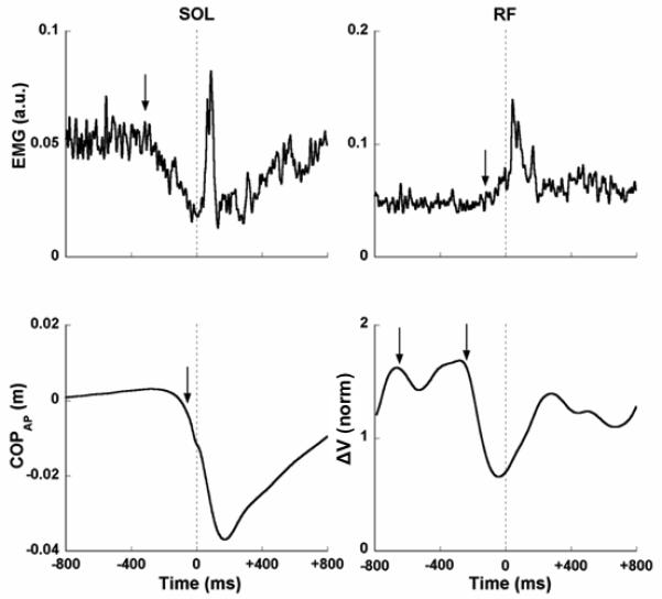
EMG traces for RF and Sol muscles, COP_AP displacements and synergy index are shown for a representative subject. Vertical dashed line at the center of the each panel corresponds to time zero, t₀ (the time of perturbation). The arrows in EMG panels represent the instant in time where the magnitude of the EMG exceeded the baseline value ± 2 standard deviations. Note the two arrows that reflect two moments of time that belong to EPA and APA. The arrow in COP_AP panel represents the instant in time where the magnitude of COP_AP crossed 5 mm from the baseline. The arrows in the synergy index panel show two drops of the peaks, each of them representing EPA and APA.

Averaged across subjects timing indices with error bars for the EPA time interval are presented in Figure 6 for the results of analyses based on both phases. The timing indices appear in the order: t_ASA < t_EMG < t_MODE < t_COP for both analyses based on the data in Phase-1 and in Phase-2. One-way ANOVA with the factor Time confirmed its main effect for both Phase-1 [F_(3,24) = 71.1, p < 0.001] and Phase-2 [F_(3,24) = 94.5, p < 0.001] based analyses. Post-hoc analyses confirmed significant differences between all the timing indices (p < 0.05), with the exception of t_MODE and t_EMG, where there were no differences, in both analyses.

Figure 6.

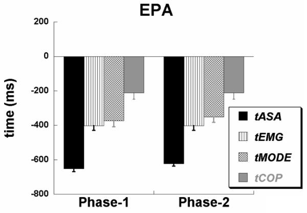
Early postural adjustments (EPA) averaged across the participants with standard error bars are shown for Phase-1 and Phase-2 analyses. Note that both the analyses produced similar early changes in the synergy index, EMGs, M-modes, and COP_AP. We present only one value for t_COP and it is included in the EPA time interval because t_COP for the two third of subjects was in the time interval before −200ms with respect to the time of perturbation, t₀. Note also that the order of their appearance is: t_ASA < t_EMG < t_MODE < t_COP.

Averaged across subjects timing indices with error bars for the APA time interval are presented in Figure 7 for both Phase-1 and Phase-2 analyses. Note, that similarly to EPA time interval, the timing indices appear in the order: t_ASA < t_EMG < t_MODE for both analyses based on the data in Phase-1 and in Phase-2. One-way ANOVA with the factor Time showed a significant main effect [F_(2,16) = 5.6, p < 0.05] and the post-hoc analysis showed a significant difference between t_ASA and t_MODE (p < 0.05) in the Phase-1 based analysis. However, one-way ANOVA based on the Phase-2 analysis did not show significant difference.

Figure 7.

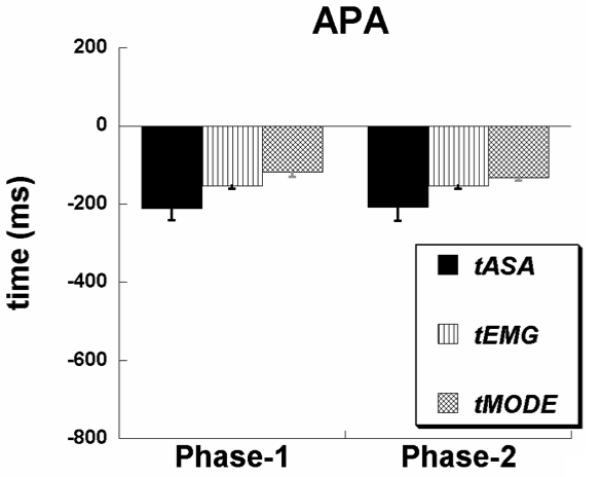
Later postural adjustments (APA) averaged across the participants with standard error bars are shown for Phase-1 and Phase-2 analyses. Note that both the analyses produced similar early changes in the synergy index, EMGs and M-modes. Note also that the order of their appearance is: t_ASA < t_EMG < t_MODE..

DISCUSSION

Our observations support the general theoretical scheme on postural preparation to action described briefly in the Introduction. In particular, the results have shown two stages of postural adjustments prior to the impact of the pendulum that produced a postural perturbation (Hypothesis #1). The early postural adjustments (EPAs) were seen in EMG signals about 300-400 ms prior to the perturbation time (t₀), while the anticipatory postural adjustments (APAs) were seen about 100 ms prior to t₀ (similarly to earlier studies reviewed by (Massion 1992). In both phases, EMG changes led to shifts of the center of pressure displacement in the anterior-posterior direction (COP_AP). In each stage, changes in the averaged across trials EMG signals were preceded by a drop in the index of a multi-M-mode synergy stabilizing the COP_AP trajectory (anticipatory synergy adjustments, ASAs, cf. Hypothesis #2). We used the data from two phases to identify the elemental variables for the analysis of synergies. Both methods produced similar results with respect to the overall pattern and relative timing of ASAs (Hypothesis #3). Further, we put the results into a single scheme of postural control based on the idea of control with referent body configurations (Feldman and Levin 1995; Feldman et al. 2007).

Posture and movement within the referent configuration hypothesis

The referent configuration hypothesis is a relatively recent development of the equilibrium-point hypothesis (EP-hypothesis, (Feldman 1986)). For the purposes of this discussion, we assume that the control system is hierarchical with the highest level producing time profiles of control variables based on the task, and the lowest level representing muscles with their motoneuronal pools and feedback loops from peripheral receptors (Latash 2010b). One should keep in mind, however, that no computations are assumed to be performed by any of the involved neuronal structures, and the hypothesized control variables are not pre-computed by some “internal models” (for a review see (Shadmehr and Wise 2005) but reflect physical processes that we currently have poor understanding of.

Thresholds of activation of neuronal pools are used as control variables by the sub-systems within the assumed hierarchy to set sequences of equilibrium states of the body interacting with the external force field. The interactions with the environment and also within the body, both mechanical and mediated by feedback loops, are directed at producing minimal muscle activation given the constraints imposed by the body anatomy and the environment. When a set of control variables remains unchanged in a steady external force field, the system “body+environment” reaches an equilibrium (a postural state) while changes in either control variables or external forces produce movement to a new equilibrium.

Recently, the idea of control with referent configurations has been coupled with an idea of multi-element synergies defined as neural organizations stabilizing salient performance variables (Latash and Zatsiorsky 2009; Latash 2010a; Latash et al. 2010a). Any action performed by a redundant motor system, that is a system with the number of variables produced by its elements (elemental variables) higher than the number of constraints imposed by typical tasks (Bernstein 1967), can be described with two characteristics. First, when a person performs an action a few times, a limited number of combinations of elemental variables are observed; such average across trials patterns have been addressed as sharing patterns (Li et al. 1998). Second, elemental variables can deviate from an average sharing pattern and co-vary across repetitive trials to keep values of some performance variables relatively unchanged; these have been addressed as error compensation (Latash et al. 1998) or flexibility and quantified using the framework of the uncontrolled manifold (UCM) hypothesis (Scholz and Schoner 1999); reviewed in (Latash et al. 2002; Latash et al. 2007). The UCM hypothesis assumes that the neural controller works within a multi-dimensional space of elemental variables and organizes in that space a sub-space (the UCM) corresponding to a desired fixed value of a performance variable to which the elemental variables contribute. Analysis of synergies involves quantifying variance of elemental variables across repetitive trials within the UCM (V_UCM) and orthogonal to the UCM (V_ORT).

Within the referent configuration hypothesis, the trademark of a synergy (V_UCM > V_ORT) may emerge as a reflection of the hierarchical organization of the control system and the nature of control variables. Indeed, an input from a hierarchically higher level specifies referent values for a handful of important variables (a referent configuration) while the few-to-many mapping performed by the lower level(s) naturally produces multiple combinations of elemental variables that are all compatible with the same referent configuration. As a result, variance across trials of the important variables is relatively low (corresponding to low V_ORT) while variance of the elemental variables may be high (resulting in high V_UCM). This interpretation has received support in a few recent studies (Pilon et al. 2007; Latash 2010a).

At each level, control variables may be viewed as specifying two features of the controlled system, its equilibrium state (given an external force field) and its resistance to possible changes in the force field. At a single-joint level, such two variables have been introduced as reciprocal command and co-activation command, r-command and c-command (Feldman 1980; Feldman and Latash 1982). At higher hierarchical levels, analogous variables have been introduced (R-command and C-command, (Latash et al. 2010b). For example, if a person moves the endpoint of a multi-joint limb, C-command will effectively change muscle co-contraction with no or small effects on endpoint coordinates while R-command would produce movement of the endpoint.

Within this scheme, postural adjustments can involve changes in both R- and C-commands. The former would produce a body sway towards a new equilibrium state and result in a net shift of the center of pressure. The latter may lead to parallel changes in the activation levels within agonist-antagonist muscle pairs (as in (Slijper and Latash 2000; Li and Aruin 2007)) and also produce changes in the co-variation of elemental variables corresponding to an unchanged, or minimally changed, posture. In our experiment, we observed early postural adjustments (EPAs) that produced COP_AP shifts after a very long time delay, compatible with the idea that they reflected primarily changes in the C-command. In contrast, COP_AP shifts during APAs have been described at much shorter time delays, about 50 ms (Li and Aruin 2007; Santos et al. 2010), which suggests that APAs are associated with changes in the R-command.

Synergic postural control and its feed-forward adjustments

The idea of synergic multi-muscle control of vertical posture has been gaining popularity lately (d’Avella et al. 2003; Krishnamoorthy et al. 2003b; Ting and Macpherson 2005; Torres-Oviedo and Ting 2007) despite a few papers that question the utility of the notion of muscle synergy (Tresch and Jarc 2009; Valero-Cuevas et al. 2009). A number of research groups have been using matrix factorization methods, such as principal component analysis, with and without factor extraction, and non-negative matrix factorization, to identify muscle groups with a close to parallel scaling of activation within a group (for a review see (Ting and Chvatal 2010). Such muscle groups have been addressed as synergies by some researchers (d’Avella et al. 2003; Ivanenko et al. 2005; Ting and Macpherson 2005; Torres-Oviedo et al. 2006; Ting 2007) while others view them as elemental variables (muscle modes or M-modes) manipulated by the controller in a synergic way (Krishnamoorthy et al. 2003a; Krishnamoorthy et al. 2003b; Danna-Dos-Santos et al. 2007; Klous et al. 2010, 2011). Within the latter approach, gains at such M-modes co-vary across repetitive trials to stabilize values or time profiles of potentially important performance variables, such as COP_AP coordinate and shear force magnitude (Danna-Dos-Santos et al. 2007; Klous et al. 2010).

In other words, the latter approach views the multi-muscle control of posture as involving two hierarchical levels: At the lower level, muscles are organized into M-modes while at the higher level magnitudes of M-modes co-vary to produce stable desired action. This approach fits the idea of control with referent configurations. In most earlier studies sets of M-modes were described corresponding to muscle activation patterns that effectively moved the body forward or backwards, so-called “push-back” and “push-forward” M-modes (Krishnamoorthy et al. 2003a; Krishnamoorthy et al. 2003b; Danna-Dos-Santos et al. 2007). Such sets of M-modes naturally reflect changes in the R-command. Different sets of M-modes have been described in challenging conditions and when unusual motor tasks were performed by a standing person (Krishnamoorthy et al. 2004; Asaka et al. 2008; Danna-Dos-Santos et al. 2008). Such M-modes involved parallel scaling of activation within agonist-antagonist muscle pairs, suggesting changes in the C-command. In our experiment, with a rather challenging semi-squat posture, the most common M-modes were joint-specific and frequently involved co-contraction patterns (see Table 2). Analysis of changes in the body configuration under the action of the M-modes suggest direct relation to the notion of eigenmovements (Alexandrov et al. 2001) based on decomposition of the equation of motion of a three-link inverted pendulum in two dimensions.

Synergies stabilizing COP displacements and shear forces have been described in several earlier studies (Krishnamoorthy et al. 2003b; Danna-Dos-Santos et al. 2007; Robert et al. 2008b; Klous et al. 2010). Our current study is unique in documenting anticipatory changes in indices of such synergies in preparation to a perturbation. Until now, such synergic adjustments (ASAs) have only been reported in multi-digit studies (Olafsdottir et al. 2005; Shim et al. 2005; Kim et al. 2006; Shim et al. 2006) and they have been assumed to reflect purposeful destabilization of a performance variable, such as total force and total moment of force, in preparation to its quick change. In our study, there were typically strong synergies stabilizing COP_AP at steady-state. Prior to any change in indices of muscle activation (EMGs or M-modes), a drop in the synergy index took place. These ASAs reflecting changes in co-variation of M-mode gains were seen 50-200 ms prior to any change in M-mode magnitudes (or EMG magnitudes) that could be detected in averaged across trials signals.

The different timing of changes in the indices of co-variation and average magnitudes of M-modes (Figure 6) corroborate the idea of two types of control variables involved in the control of a redundant system (Latash et al. 2007). One group of control variables defines averaged across trials patterns of elemental variables (sharing), while the other group defines co-variation of those same elemental variables across all individual trials.

Two stages of postural preparation to action

There were both similarities and differences in the organization of postural adjustments during EPAs and APAs. The similarities involved an early drop in the multi-M-mode synergy stabilizing COP_AP, which is ASA. The most striking differences were in the timing of the EPAs and APAs with respect to the impact time and in the very long electromechanical delay (EMD) between the first detectable changes in EMG and M-mode signals and the first detectable COP_AP shift during the EPAs. Earlier studies of APAs reported EMD values on the order of about 50 ms (Cavanagh and Komi 1979; Howatson et al. 2009). Such magnitudes are also compatible with studies of EMD in a variety of tasks (reviewed in (Corcos et al. 1992)). The EMD of about 200 ms during the EPAs suggests that during that stage of postural adjustment, changes in the muscle activation patterns were organized to produce a relatively small COP_AP shift while adjusting the posture without producing a net COP_AP shift. This view fits the idea of producing EPAs primarily with changes in the C-command.

EPAs have been known for a long time. Indeed, studies of postural adjustments to stepping reported COP shifts starting several hundred ms prior to the take-off of the leading foot (Elble et al. 1994; Lepers and Breniere 1995; Couillandre et al. 2002). However, those adjustments have been addressed as APAs. Our study suggests that EPAs and APAs are two separate phenomena of postural preparation and, moreover, they can be observed within a single trial at different times with respect to the perturbation time.

In our study, EPAs were associated with small, delayed COP_AP changes. So, they can be interpreted as postural adjustments with minimal changes in the net mechanical variables exerted on the environment, while their main purpose is to adjust posture for preparation to an expected (planned) perturbation (action). In contrast, APAs were associated with visible COP_AP shifts at a time delay of about 50 ms (we did not quantify those because they were superimposed on continuing COP_AP shifts initiated during the EPAs), similarly to earlier reports (Li and Aruin 2007; Santos et al. 2010). Hence, APAs may be interpreted as changes in the postural muscle activation with the purpose to produce net forces and moments of force counteracting mechanical effects on the expected perturbation on vertical posture (cf. (Bouisset and Zattara 1987; Ramos and Stark 1990)).

Three components of postural preparation to action

Each of the two stages was characterized by three components, changes in co-variation of M-modes magnitudes (ASAs), changes in individual muscle activation levels and M-mode magnitudes seen in averaged across trials data, and changes in mechanical variables (reflected in COP_AP in our study). The three components followed each other in the mentioned order.

Consider the findings within the described earlier scheme of synergic control with referent configurations (Figure 8). At the highest hierarchical level, task-related input defines sub-threshold depolarization of a target neural pool (N1). Given the external force field, this input also defines a referent configuration (a set of referent values of important peripheral variables, COP_AP in our case). N1 is driven by (processed within the central nervous system) afferent feedback signals related to the mismatch between the current COP_AP value and its referent value. Its activation continues until actual COP_AP equals the referent one. The output of N1 projects on a higher-dimensional set of neurons that define changes in elemental variables at that intermediate level. Based on an earlier study (Robert et al. 2008b), we assume that these variables represent changes in joint referent configuration corresponding to the eigen-movements introduced by (Alexandrov et al. 2001) and reflected in the composition of M-modes defined in our study. The output of this level serves as an input into a lower level. We assume that the lowest level represent individual muscle control, with referent configurations corresponding to λs (thresholds of the tonic stretch reflex, see (Feldman 1966; Feldman and Orlovsky 1972; Feldman 1986). Theoretically, synergic relationships may be expected at both few-to-many transformations, TASK => M-modes and M-mode => EMGs based on the shown feedback loops. The tonic stretch reflex may also be viewed as a synergy stabilizing the equilibrium-point of the system “muscle+load” (Latash et al. 2007).

Figure 8.

A schematic representation of synergic control with referent configurations. The task defines an input (subthreshold depolarization) into the highest level of the hierarchy (N1); in combination with the external force field, it also defines time evolution of the referent configuration. The output at each level of the hierarchy projects onto a redundant set of elements; their combined output is sensed by a sensory neuron and projected back to the input. N1 projects onto a set of neuronal pools that define magnitudes of M-modes, while each of those pools projects onto a redundant set of α-motoneuronal pools. The final synergic relationship is ensured by the mechanism of the tonic stretch reflex. As a result, there is a chain of local feedback loops stabilizing the combined action of corresponding redundant sets of elements (ensuring synergies at those levels) and a global feedback loop from peripheral sensors that ensures that the system as a whole is attracted to its referent configuration.

Within the scheme illustrated in Figure 8, changes in the synergy index without visible changes in the averaged across trials M-mode magnitudes (and EMGs) may be produced by changes in the feedback gain of the upper loop (analogous to changes in the feedback gain matrix in (Latash et al. 2007). This is the cause of ASAs. Changes in the averaged across trials EMG and M-mode signals may be generated by a change in the TASK input without changes in the referent value of the important performance variable (COP_AP). This is analogous to modifying the C-command (see earlier) without changes in the R-command. We suggest that such changes form the basis of the EPAs, i.e. postural adjustments not associated with major changes in COP_AP. ASAs are generated in a similar fashion, but changes in both C- and R-command are likely at the upper level of the hierarchy leading to the generation of net mechanical effects.

We would like to emphasize that the relative timing of the different variables discovered in the study is not trivial (although reasonable). First, t_ASA does not have to occur before any other timing indices. In fact, ASA is a relatively novel phenomenon, and it was not obvious upfront that any consistent changes in the index of synergy would occur during postural adjustments. If such changes do occur, they do not have to happen before changes in the averaged profiles of EMGs (or other variables). Second, t_EMG and t_MODE were defined using a mean ± SD criterion. One may expect t_EMG to occur priot to t_MODE because t_EMG was defined as the earliest EMG change but, given the definition of the timing indices, this is not guaranteed. Shifts of the COP are expected to happen after t_EMG but only if the activation levels of all the muscles that contribute to COP shifts are recorded. Since this is practically impossible, t_COP may happen prior to t_EMG.

To summarize, our results fit the idea of posture/movement control with referent body configurations. They suggest different, specific processes underlying the two stages and three components of postural preparation to perturbation/action.

REFERENCES

- Alexandrov AV, Frolov AA, Massion J. Biomechanical analysis of movement strategies in human forward trunk bending. II. Experimental study. Biol Cybern. 2001;84:435–443. doi: 10.1007/PL00007987. [DOI] [PubMed] [Google Scholar]
- Aruin AS, Latash ML. The role of motor action in anticipatory postural adjustments studied with self-induced and externally triggered perturbations. Exp Brain Res. 1995;106:291–300. doi: 10.1007/BF00241125. [DOI] [PubMed] [Google Scholar]
- Aruin AS, Latash ML. Anticipatory postural adjustments during self-initiated perturbations of different magnitude triggered by a standard motor action. Electroencephalogr Clin Neurophysiol. 1996;101:497–503. doi: 10.1016/s0013-4694(96)95219-4. [DOI] [PubMed] [Google Scholar]
- Asaka T, Wang Y, Fukushima J, Latash ML. Learning effects on muscle modes and multi-mode postural synergies. Exp Brain Res. 2008;184:323–338. doi: 10.1007/s00221-007-1101-2. [DOI] [PMC free article] [PubMed] [Google Scholar]
- Belenkiy V, Gurfinkel V, Pal’tsev Y. Elements of control of voluntary movements. Biofizika. 1967;10:135–141. [PubMed] [Google Scholar]
- Bernstein N. Pergamon Press; London: 1967. The coordination and regulation of movements. [Google Scholar]
- Bouisset S, Zattara M. Biomechanical study of the programming of anticipatory postural adjustments associated with voluntary movement. J Biomechanics. 1987;20:735–742. doi: 10.1016/0021-9290(87)90052-2. [DOI] [PubMed] [Google Scholar]
- Cavanagh PR, Komi PV. Electromechanical delay in human skeletal muscle under concentric and eccentric contractions. Eur J Appl Physiol Occup Physiol. 1979;42:159–163. doi: 10.1007/BF00431022. [DOI] [PubMed] [Google Scholar]
- Corcos DM, Gottlieb GL, Latash ML, Almeida GL, Agarwal GC. Electromechanical delay: An experimental artifact. J Electromyogr Kinesiol. 1992;2:59–68. doi: 10.1016/1050-6411(92)90017-D. [DOI] [PubMed] [Google Scholar]
- Cordo PJ, Nashner LM. Properties of postural adjustments associated with rapid arm movements. J Neurophysiol. 1982;47:287–302. doi: 10.1152/jn.1982.47.2.287. [DOI] [PubMed] [Google Scholar]
- Couillandre A, Maton B, Breniere Y. Voluntary toe-walking gait initiation: electromyographical and biomechanical aspects. Exp Brain Res. 2002;147:313–321. doi: 10.1007/s00221-002-1254-y. [DOI] [PubMed] [Google Scholar]
- Crenna P, Frigo C. A motor programme for the initiation of forward-oriented movements in humans. J Physiol. 1991;437:635–653. doi: 10.1113/jphysiol.1991.sp018616. [DOI] [PMC free article] [PubMed] [Google Scholar]
- d’Avella A, Saltiel P, Bizzi E. Combinations of muscle synergies in the construction of a natural motor behavior. Nat Neurosci. 2003;6:300–308. doi: 10.1038/nn1010. [DOI] [PubMed] [Google Scholar]
- Danna-Dos-Santos A, Degani AM, Latash ML. Flexible muscle modes and synergies in challenging whole-body tasks. Exp Brain Res. 2008;189:171–187. doi: 10.1007/s00221-008-1413-x. [DOI] [PMC free article] [PubMed] [Google Scholar]
- Danna-Dos-Santos A, Slomka K, Zatsiorsky VM, Latash ML. Muscle modes and synergies during voluntary body sway. Exp Brain Res. 2007;179:533–550. doi: 10.1007/s00221-006-0812-0. [DOI] [PubMed] [Google Scholar]
- De Wolf S, Slijper H, Latash ML. Anticipatory postural adjustments during self-paced and reaction-time movements. Exp Brain Res. 1998;121:7–19. doi: 10.1007/s002210050431. [DOI] [PubMed] [Google Scholar]
- Elble RJ, Moody C, Leffler K, Sinha R. The initiation of normal walking. Mov Disord. 1994;9:139–146. doi: 10.1002/mds.870090203. [DOI] [PubMed] [Google Scholar]
- Feldman AG. On the functional tuning of the nervous system in movement control or preservation of stationary pose. II. Adjustable parameters in muscles. Biofizika. 1966;11:498–508. [PubMed] [Google Scholar]
- Feldman AG. Superposition of motor programs--I. Rhythmic forearm movements in man. Neuroscience. 1980;5:81–90. doi: 10.1016/0306-4522(80)90073-1. [DOI] [PubMed] [Google Scholar]
- Feldman AG. Once more on the equilibrium-point hypothesis (lambda model) for motor control. J Mot Behav. 1986;18:17–54. doi: 10.1080/00222895.1986.10735369. [DOI] [PubMed] [Google Scholar]
- Feldman AG, Goussev V, Sangole A, Levin MF. Threshold position control and the principle of minimal interaction in motor actions. Prog Brain Res. 2007;165:267–281. doi: 10.1016/S0079-6123(06)65017-6. [DOI] [PubMed] [Google Scholar]
- Feldman AG, Latash ML. Afferent and efferent components of joint position sense; interpretation of kinaesthetic illusion. Biol Cybern. 1982;42:205–214. doi: 10.1007/BF00340077. [DOI] [PubMed] [Google Scholar]
- Feldman AG, Levin MF. The Origin and Use of Positional Frames of Reference in Motor Control. Behavioral and Brain Sciences. 1995;18:723–744. [Google Scholar]
- Feldman AG, Orlovsky GN. The influence of different descending systems on the tonic stretch reflex in the cat. Exp Neurol. 1972;37:481–494. doi: 10.1016/0014-4886(72)90091-x. [DOI] [PubMed] [Google Scholar]
- Hair JF, Anderson RE, Tatham RL, Black WC. Factor analysis. In: Borkowski D, editor. Multivariate data analysis. Prentice Hall; Englewood Cliffs: 1995. pp. 364–404. [Google Scholar]
- Halliday SE, Winter DA, Frank JS, Patla AE, Prince F. The initiation of gait in young, elderly, and Parkinson’s disease subjects. Gait Posture. 1998;8:8–14. doi: 10.1016/s0966-6362(98)00020-4. [DOI] [PubMed] [Google Scholar]
- Hirschfeld H, Forssberg H. Phase-dependent modulations of anticipatory postural activity during human locomotion. J Neurophysiol. 1991;66:12–19. doi: 10.1152/jn.1991.66.1.12. [DOI] [PubMed] [Google Scholar]
- Howatson G, Glaister M, Brouner J, van Someren KA. The reliability of electromechanical delay and torque during isometric and concentric isokinetic contractions. J Electromyogr Kinesiol. 2009;19:975–979. doi: 10.1016/j.jelekin.2008.02.002. [DOI] [PubMed] [Google Scholar]
- Ivanenko YP, Cappellini G, Dominici N, Poppele RE, Lacquaniti F. Coordination of locomotion with voluntary movements in humans. J Neurosci. 2005;25:7238–7253. doi: 10.1523/JNEUROSCI.1327-05.2005. [DOI] [PMC free article] [PubMed] [Google Scholar]
- Ivanenko YP, Wright WG, Gurfinkel VS, Horak F, Cordo P. Interaction of involuntary post-contraction activity with locomotor movements. Exp Brain Res. 2006;169:255–260. doi: 10.1007/s00221-005-0324-3. [DOI] [PMC free article] [PubMed] [Google Scholar]
- Jacobs JV, Nutt JG, Carlson-Kuhta P, Stephens M, Horak FB. Knee trembling during freezing of gait represents multiple anticipatory postural adjustments. Exp Neurol. 2009;215:334–341. doi: 10.1016/j.expneurol.2008.10.019. [DOI] [PMC free article] [PubMed] [Google Scholar]
- Kim SW, Shim JK, Zatsiorsky VM, Latash ML. Anticipatory adjustments of multi-finger synergies in preparation for self-triggered perturbations. Exp Brain Res. 2006;174:604–612. doi: 10.1007/s00221-006-0505-8. [DOI] [PubMed] [Google Scholar]
- Klous M, Danna-dos-Santos A, Latash ML. Multi-muscle synergies in a dual postural task: evidence for the principle of superposition. Exp Brain Res. 2010;202:457–471. doi: 10.1007/s00221-009-2153-2. [DOI] [PMC free article] [PubMed] [Google Scholar]
- Klous M, Mikulic P, Latash ML. Two aspects of feed-forward postural control: Anticipatory postural adjustments and anticipatory synergy adjustments. J Neurophysiol. 2011 doi: 10.1152/jn.00665.2010. in press. [DOI] [PMC free article] [PubMed] [Google Scholar]
- Krishnamoorthy V, Goodman S, Zatsiorsky V, Latash ML. Muscle synergies during shifts of the center of pressure by standing persons: identification of muscle modes. Biol Cybern. 2003a;89:152–161. doi: 10.1007/s00422-003-0419-5. [DOI] [PubMed] [Google Scholar]
- Krishnamoorthy V, Latash ML. Reversals of anticipatory postural adjustments during voluntary sway in humans. J Physiol. 2005;565:675–684. doi: 10.1113/jphysiol.2005.084772. [DOI] [PMC free article] [PubMed] [Google Scholar]
- Krishnamoorthy V, Latash ML, Scholz JP, Zatsiorsky VM. Muscle synergies during shifts of the center of pressure by standing persons. Exp Brain Res. 2003b;152:281–292. doi: 10.1007/s00221-003-1574-6. [DOI] [PubMed] [Google Scholar]
- Krishnamoorthy V, Latash ML, Scholz JP, Zatsiorsky VM. Muscle modes during shifts of the center of pressure by standing persons: effect of instability and additional support. Exp Brain Res. 2004;157:18–31. doi: 10.1007/s00221-003-1812-y. [DOI] [PubMed] [Google Scholar]
- Kung UM, Horlings CG, Honegger F, Allum JH. Incorporating voluntary unilateral knee flexion into balance corrections elicited by multi-directional perturbations to stance. Neuroscience. 2009;163:466–481. doi: 10.1016/j.neuroscience.2009.06.009. [DOI] [PubMed] [Google Scholar]
- Latash ML. Motor synergies and the equilibrium-point hypothesis. Motor Control. 2010a;14:294–322. doi: 10.1123/mcj.14.3.294. [DOI] [PMC free article] [PubMed] [Google Scholar]
- Latash ML. Stages in learning motor synergies: a view based on the equilibrium-point hypothesis. Hum Mov Sci. 2010b;29:642–654. doi: 10.1016/j.humov.2009.11.002. [DOI] [PMC free article] [PubMed] [Google Scholar]
- Latash ML, Friedman J, Kim SW, Feldman AG, Zatsiorsky VM. Prehension synergies and control with referent hand configurations. Exp Brain Res. 2010a;202:213–229. doi: 10.1007/s00221-009-2128-3. [DOI] [PMC free article] [PubMed] [Google Scholar]
- Latash ML, Gelfand IM, Li ZM, Zatsiorsky VM. Changes in the force-sharing pattern induced by modifications of visual feedback during force production by a set of fingers. Exp Brain Res. 1998;123:255–262. doi: 10.1007/s002210050567. [DOI] [PubMed] [Google Scholar]
- Latash ML, Levin MF, Scholz JP, Schoner G. Motor control theories and their applications. Medicina (Kaunas) 2010b;46:382–392. [PMC free article] [PubMed] [Google Scholar]
- Latash ML, Scholz JP, Schoner G. Motor control strategies revealed in the structure of motor variability. Exerc Sport Sci Rev. 2002;30:26–31. doi: 10.1097/00003677-200201000-00006. [DOI] [PubMed] [Google Scholar]
- Latash ML, Scholz JP, Schoner G. Toward a new theory of motor synergies. Motor Control. 2007;11:276–308. doi: 10.1123/mcj.11.3.276. [DOI] [PubMed] [Google Scholar]
- Latash ML, Zatsiorsky VM. Multi-finger prehension: control of a redundant mechanical system. Adv Exp Med Biol. 2009;629:597–618. doi: 10.1007/978-0-387-77064-2_32. [DOI] [PubMed] [Google Scholar]
- Lepers R, Breniere Y. The role of anticipatory postural adjustments and gravity in gait initiation. Exp Brain Res. 1995;107:118–124. doi: 10.1007/BF00228023. [DOI] [PubMed] [Google Scholar]
- Li X, Aruin AS. The effect of short-term changes in the body mass on anticipatory postural adjustments. Exp Brain Res. 2007;181:333–346. doi: 10.1007/s00221-007-0931-2. [DOI] [PubMed] [Google Scholar]
- Li ZM, Latash ML, Zatsiorsky VM. Force sharing among fingers as a model of the redundancy problem. Exp Brain Res. 1998;119:276–286. doi: 10.1007/s002210050343. [DOI] [PubMed] [Google Scholar]
- Massion J. Movement, posture and equilibrium: interaction and coordination. Prog Neurobiol. 1992;38:35–56. doi: 10.1016/0301-0082(92)90034-c. [DOI] [PubMed] [Google Scholar]
- Nana-Ibrahim S, Vieilledent S, Leroyer P, Viale F, Zattara M. Target size modifies anticipatory postural adjustments and subsequent elementary arm pointing. Exp Brain Res. 2008;184:255–260. doi: 10.1007/s00221-007-1178-7. [DOI] [PubMed] [Google Scholar]
- Olafsdottir H, Yoshida N, Zatsiorsky VM, Latash ML. Anticipatory covariation of finger forces during self-paced and reaction time force production. Neurosci Lett. 2005;381:92–96. doi: 10.1016/j.neulet.2005.02.003. [DOI] [PMC free article] [PubMed] [Google Scholar]
- Pilon JF, De Serres SJ, Feldman AG. Threshold position control of arm movement with anticipatory increase in grip force. Exp Brain Res. 2007;181:49–67. doi: 10.1007/s00221-007-0901-8. [DOI] [PubMed] [Google Scholar]
- Ramos CF, Stark LW. Postural maintenance during fast forward bending: a model simulation experiment determines the “reduced trajectory”. Exp Brain Res. 1990;82:651–657. doi: 10.1007/BF00228807. [DOI] [PubMed] [Google Scholar]
- Robert T, Zatsiorsky VM, Latash ML. Multi-muscle synergies in an unusual postural task: quick shear force production. Exp Brain Res. 2008a doi: 10.1007/s00221-008-1299-7. [DOI] [PMC free article] [PubMed] [Google Scholar]
- Robert T, Zatsiorsky VM, Latash ML. Multi-muscle synergies in an unusual postural task: quick shear force production. Exp Brain Res. 2008b;187:237–253. doi: 10.1007/s00221-008-1299-7. [DOI] [PMC free article] [PubMed] [Google Scholar]
- Saltiel P, Wyler-Duda K, D’Avella A, Tresch MC, Bizzi E. Muscle synergies encoded within the spinal cord: evidence from focal intraspinal NMDA iontophoresis in the frog. J Neurophysiol. 2001;85:605–619. doi: 10.1152/jn.2001.85.2.605. [DOI] [PubMed] [Google Scholar]
- Santos MJ, Aruin AS. Role of lateral muscles and body orientation in feedforward postural control. Exp Brain Res. 2008;184:547–559. doi: 10.1007/s00221-007-1123-9. [DOI] [PubMed] [Google Scholar]
- Santos MJ, Kanekar N, Aruin AS. The role of anticipatory postural adjustments in compensatory control of posture: 1. Electromyographic analysis. J Electromyogr Kinesiol. 2010;20:388–397. doi: 10.1016/j.jelekin.2009.06.006. [DOI] [PubMed] [Google Scholar]
- Scholz JP, Schoner G. The uncontrolled manifold concept: identifying control variables for a functional task. Exp Brain Res. 1999;126:289–306. doi: 10.1007/s002210050738. [DOI] [PubMed] [Google Scholar]
- Shadmehr R, Wise SP. The computational neurobiology of reaching and pointing. MIT Press; Cambridge, MA: 2005. [Google Scholar]
- Shim JK, Olafsdottir H, Zatsiorsky VM, Latash ML. The emergence and disappearance of multi-digit synergies during force-production tasks. Exp Brain Res. 2005;164:260–270. doi: 10.1007/s00221-005-2248-3. [DOI] [PMC free article] [PubMed] [Google Scholar]
- Shim JK, Park J, Zatsiorsky VM, Latash ML. Adjustments of prehension synergies in response to self-triggered and experimenter-triggered load and torque perturbations. Exp Brain Res. 2006;175:641–653. doi: 10.1007/s00221-006-0583-7. [DOI] [PMC free article] [PubMed] [Google Scholar]
- Slijper H, Latash M. The effects of instability and additional hand support on anticipatory postural adjustments in leg, trunk, and arm muscles during standing. Exp Brain Res. 2000;135:81–93. doi: 10.1007/s002210000492. [DOI] [PubMed] [Google Scholar]
- Stapley P, Pozzo T, Grishin A. The role of anticipatory postural adjustments during whole body forward reaching movements. Neuroreport. 1998;9:395–401. doi: 10.1097/00001756-199802160-00007. [DOI] [PubMed] [Google Scholar]
- ing LH. Dimensional reduction in sensorimotor systems: a framework for understanding muscle coordination of posture. Prog Brain Res. 2007;165:299–321. doi: 10.1016/S0079-6123(06)65019-X. [DOI] [PMC free article] [PubMed] [Google Scholar]
- Ting LH, Chvatal SA. Decomposing Muscle Activity in Motor Tasks. In: Danion F, Latash ML, editors. Motor Control. Theories, Experiments and Applications. Oxford University Press; New York: 2010. pp. 102–138. [Google Scholar]
- Ting LH, Macpherson JM. A limited set of muscle synergies for force control during a postural task. J Neurophysiol. 2005;93:609–613. doi: 10.1152/jn.00681.2004. [DOI] [PubMed] [Google Scholar]
- Torres-Oviedo G, Macpherson JM, Ting LH. Muscle synergy organization is robust across a variety of postural perturbations. J Neurophysiol. 2006;96:1530–1546. doi: 10.1152/jn.00810.2005. [DOI] [PubMed] [Google Scholar]
- Torres-Oviedo G, Ting LH. Muscle synergies characterizing human postural responses. J Neurophysiol. 2007;98:2144–2156. doi: 10.1152/jn.01360.2006. [DOI] [PubMed] [Google Scholar]
- Tresch MC, Jarc A. The case for and against muscle synergies. Curr Opin Neurobiol. 2009;19:601–607. doi: 10.1016/j.conb.2009.09.002. [DOI] [PMC free article] [PubMed] [Google Scholar]
- Valero-Cuevas FJ, Venkadesan M, Todorov E. Structured variability of muscle activations supports the minimal intervention principle of motor control. J Neurophysiol. 2009;102:59–68. doi: 10.1152/jn.90324.2008. [DOI] [PMC free article] [PubMed] [Google Scholar]
- Winter DA, Prince F, Frank JS, Powell C, Zabjek KF. Unified theory regarding A/P and M/L balance in quiet stance. J Neurophysiol. 1996;75:2334–2343. doi: 10.1152/jn.1996.75.6.2334. [DOI] [PubMed] [Google Scholar]