Challenges of Guarantee-Time Bias

Abstract

The potential for guarantee-time bias (GTB), also known as immortal time bias, exists whenever an analysis that is timed from enrollment or random assignment, such as disease-free or overall survival, is compared across groups defined by a classifying event occurring sometime during follow-up. The types of events associated with GTB are varied and may include the occurrence of objective disease response, onset of toxicity, or seroconversion. However, comparative analyses using these types of events as predictors are different from analyses using baseline characteristics that are specified completely before the occurrence of any outcome event. Recognizing the potential for GTB is not always straightforward, and it can be challenging to know when GTB is influencing the results of an analysis. This article defines GTB, provides examples of GTB from several published articles, and discusses three analytic techniques that can be used to remove the bias: conditional landmark analysis, extended Cox model, and inverse probability weighting. The strengths and limitations of each technique are presented. As an example, we explore the effect of bisphosphonate use on disease-free survival (DFS) using data from the BIG (Breast International Group) 1-98 randomized clinical trial. An analysis using a naive approach showed substantial benefit for patients who received bisphosphonate therapy. In contrast, analyses using the three methods known to remove GTB showed no statistical evidence of a reduction in risk of a DFS event with bisphosphonate therapy.

INTRODUCTION

In the context of clinical trials, the issue of guarantee-time bias (GTB) arises when an analysis that is timed from enrollment or random assignment, such as disease-free (DFS) or overall survival (OS), is compared across groups defined by a classifying event occurring sometime during follow-up. The classifying event may be as diverse as objective response to treatment, change in a biomarker, response after neoadjuvant therapy, onset of a certain type of adverse event, initiation of a subsequent or secondary treatment, or occurrence of treatment noncompliance. Patients may enter the classifying event group early or late in follow-up; however, those patients who experience the classifying event must have been undergoing follow-up long enough for the event to occur.

A classic example of GTB in oncology is its effect on analyses of survival by tumor response in phase II chemotherapy trials.^1,2 In the 1983 report by Anderson et al,¹ the authors note that “patients with prognosis and who die early in the study will not have an opportunity to enter the responder group and will guarantee poorer survival for the nonresponse group.”^1(p711)

It can be challenging for investigators to recognize when GTB is influencing the outcome of their analyses. The purpose of this article is to raise awareness of this issue so that investigators can recognize analyses in which results may be influenced by such bias.

BACKGROUND

Some of the early discussions of GTB occurred in the transplantation literature. Gail³ challenged the analysis of survival data from two studies of cardiac transplantation, suggesting that the group assignment methods that were used favored the transplantation group. He maintained that the improved survival in the transplantation group could be explained, in part, by GTB. Patients in the transplantation group were guaranteed to have survived at least until a donor was available, whereas the no-transplantation group included, by default, all patients who had died before a suitable donor could be found. This resulted in survival estimates that were exaggerated in a favorable direction for the transplantation group and in an unfavorable direction for the no-transplantation group. Figure 1 illustrates GTB based on Gail's observation.

Fig 1.

Impact of guarantee time on survival according to Gail³ transplantation model. Patients who undergo transplantation seem to have longer survival times. However, patients in the transplantation group must survive at least until donor is available (blue), and their survival reflects total time before and after transplantation (blue and gold). More favorable survival does not result from the effect of transplantation but rather from the inclusion of extra waiting time (guarantee time). By contrast, the no-transplantation group includes all patients who died before a suitable donor could be found.

GTB not only occurs in the setting of clinical trials but can also occur in observational or cohort (case-control) studies and is referred to in that literature as immortal time bias, survivor treatment selection bias, or survivor bias. Immortal time bias has even been used to explain the unexpected proposition that Oscar-winning actors live longer.⁴ In all guises, it refers to a span of time in the observation or follow-up period of a cohort when death, or the outcome under study, could not have occurred.

During immortal time, a participant is not truly immortal, but he or she must remain free of the outcome until the classifying event occurs to be included in that group. It has also been noted that in cohort studies using computerized health care databases as the source of data, immortal time bias may result from the different approaches used to form the cohorts.⁵ In this article, we use the term GTB as an umbrella term that includes immortal time bias, survivor bias, and survivor treatment selection bias.

IDENTIFYING GTB

Recognizing the potential for GTB is not always straightforward. In the initial report of the NSABP (National Surgical Adjuvant Breast and Bowel Project) B-30 trial,⁶ which evaluated chemotherapy regimens in node-positive early breast cancer, the subgroup of women with amenorrhea and estrogen receptor (ER) –negative disease was found to have improved DFS and OS, contrary to the hypothesis that chemotherapy-induced amenorrhea would influence DFS or OS only in women with ER-positive disease. This result was unexpected and, in the words of the authors, “one of the most intriguing findings of this trial.”^6(p2063)

In the NSABP B-30 trial, the classifying event, amenorrhea, was defined as at least 6 months without a menstrual period during the first 24 months of follow-up. The definition introduced the potential for GTB because DFS was measured from random assignment, but assignment into amenorrhea groups required a sufficiently long DFS interval before classification as having amenorrhea; patients with short DFS times were disproportionately allocated to the no-amenorrhea group. GTB was likely to have a much greater effect on analyses for patients with ER-negative disease, who are more likely to have early relapses, than for patients with ER-positive disease, for whom early relapses are less common. When the analysis employed techniques to remove GTB (ie, 12-month conditional landmark analysis), the effect of amenorrhea on DFS and OS continued to be observed for the ER-positive cohort, but it completely disappeared for the ER-negative cohort.⁷ Additional details regarding analytic methods to address GTB are presented in the Analytic Methods section.

We illustrate this differential change in outcome according to amenorrhea status using data from IBCSG (International Breast Cancer Study Group) 13-93 trial, a randomized phase III clinical trial in premenopausal women with lymph node–positive breast cancer.⁸ A woman was classified as amenorrheic if there was at least one report of no menses during the first five follow-up visits (15 to 18 months) after random assignment. The primary outcome of DFS was evaluated separately for women with ER-positive and ER-negative disease. In a naive analysis of DFS that did not consider the amenorrhea guarantee time (Figs 2A and 2B), women with amenorrhea had highly significant reductions in the hazards of DFS events regardless of ER status (ER positive: hazard ratio [HR], 0.45; 95% CI, 0.34 to 0.60; P < .001; ER negative: HR, 0.56; 95% CI, 0.38 to 0.81; P = .002). However, using an analytic method that removes GTB (ie, 18-month landmark analysis), a significant reduction in the risk of a DFS event was still seen in women with ER-positive disease (HR, 0.61; 95% CI, 0.43 to 0.85; P = .004) but not in women with ER-negative disease, who were more likely to have early relapses (HR, 1.38; 95% CI, 0.75 to 2.57; P = .30; Figs 2C and 2D). We see from this example that the extent to which GTB can influence results depends on the length of time needed to observe the classifying event relative to the time frame during which outcome events are likely to be observed.

Fig 2.

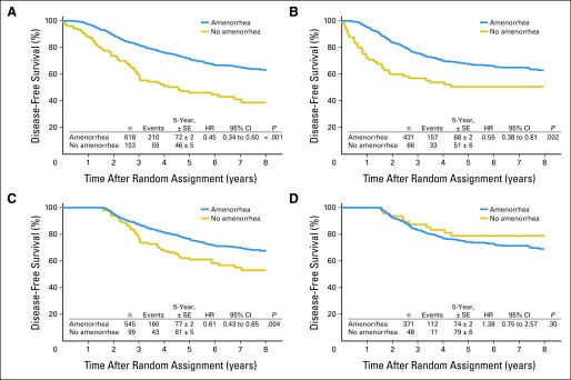
Comparisons of disease-free survival (DFS) in IBCSG (International Breast Cancer Study Group) 13-93 according to amenorrhea status using naive and 18-month landmark analyses. DFS was evaluated separately for women with (A) estrogen receptor (ER) –positive and (B) ER-negative disease. (A, B) Naive analyses showed highly significant reductions in hazards of DFS events independent of ER status. Eighteen-month landmark analyses showed significant reductions in risks of DFS events in women with (C) ER-positive disease but not in women (D) with ER-negative disease, who are more likely to experience early relapse. HR, hazard ratio.

At the 48th Annual Meeting of the American Society of Clinical Oncology in 2012, a presentation from the MA.27 trial by Shepherd et al⁹ showed that patients who used bisphosphonates at any time during study follow-up had better event-free survival than those who never used bisphosphonates. This led to our own exploration of the effect of bisphosphonate use on DFS based on data from the BIG 1-98 trial. Patients were classified as having bisphosphonate therapy if they reported use at baseline or at any follow-up visit preceding a DFS event by at least 30 days. All other patients were classified as not using bisphosphonates.

On the basis of data from the 12-year update of BIG 1-98, of 8,010 women in the intention-to-treat cohort, 981 (12%) had exposure to bisphosphonates either at the time of enrollment or during follow-up. As shown in Table 1, 567 of the 981 women began bisphosphonate therapy ≥ 36 months after starting the trial. Thus, more than half of the bisphosphonate users had to remain disease free for at least 3 years from random assignment to be classified as users, a condition of longevity that does not apply to the no-bisphosphonate group.

Table 1.

BIG 1-98: Time to Start of Bisphosphonate Therapy Based on 981 Women Reporting Bisphosphonate Use

Time Interval	Frequency	%	Cumulative Frequency
Before random assignment	22	2.2	22
At time of random assignment	85	8.7	107
After random assignment, months
0 to 12	91	9.3	198
12 to 24	99	10.1	297
24 to 36	117	12.0	414
≥ 36	567	57.8	981

Abbreviation: BIG, Breast International Group.

Recently, the US Food and Drug Administration issued a guidance document suggesting that evidence of improvement in the pathologic complete response (pCR) rate might be used to predict treatment efficacy for registration purposes because of its association with improved DFS and OS.¹⁰ Several demonstrations of this in breast cancer have been published, including a report by von Minckwitz et al.¹¹ GTB can influence results when DFS is measured from date of study enrollment, and the classifying event (pCR) is assessed several months after enrollment at the time of surgery. The magnitude of the bias may be small because the time to determine pCR is short relative to the usual time to a DFS event. However, GTB may have a larger influence on results for tumor subtypes with early relapses.

GTB can also influence an analysis that assesses outcome differences based on duration of therapy. An article by Souhami et al¹² examined the differences in outcomes according to the duration of adjuvant hormonal therapy in men with locally advanced prostate cancer who participated in the RTOG (Radiation Therapy Oncology Group) 85-31 study. The authors concluded that hormonal therapy duration of at least 5 years improved outcomes. Several commentaries from statisticians and clinicians appeared after this article was published, all of which noted the bias in the analysis. The bias resulted from the exclusion of patients who discontinued hormonal therapy because of death, disease progression, or initiation of another hormonal therapy before 5 years. Patients with shorter treatment duration tended to have earlier prostate events and deaths, and it is expected that these men would have had worse outcomes than those who remained relapse free and received therapy for at least five years. As noted by Tangen et al,¹³ “duration of therapy is simply a surrogate measure for early versus late events.”^13(pe203)

As a final example of GTB identification, we present an analysis of biomarker data from biobanked samples. In a study to assess the prevalence of KRAS mutations and their association with prognosis in patients with metastatic colorectal cancer (mCRC), Montomoli et al¹⁴ used the Danish Pathology Database to identify primary tumor specimens from patients with mCRC. KRAS mutation status was assessed and linked to patients' clinical data to obtain follow-up status and dates of first CRC diagnosis. In this study, only patients with mCRC who were receiving palliative chemotherapy during the study period were included for assessment of KRAS status, but survival time was calculated based on date of CRC diagnosis. The authors state that the survival estimates should be interpreted cautiously because survival time was calculated based on diagnosis date, but only patients who lived long enough to be eligible for KRAS testing were included. This introduced GTB and most likely overestimated survival. The example again emphasizes the significance of the timing of the classifying assessments relative to the timing of the outcome measures when considering GTB.

STATISTICAL ISSUES

Several statistical issues become important when dealing with GTB. The first is that membership in the classifying event group may change with time. As can be seen in the bisphosphonate data from BIG 1-98, the majority of bisphosphonate users began the therapy ≥ 3 years after study enrollment. These women began the trial not receiving bisphosphonate therapy and changed status ≥ 3 years later. Any naive analysis that ignores this fact would simply classify the women as bisphosphonate users or not, regardless of when the therapy began. Especially in situations in which an outcome can occur over an extended period of time, the opportunity to switch into the classifying event group is greater and can result in a larger GTB.

A second related classification issue results from early outcome events. Because all patients begin as members of the nonevent group (eg, no transplantation, without amenorrhea), those with early outcome events are not eligible to change status. This has an unfavorable effect on the outcome estimates in the nonevent group. Early events can also increase the effect of GTB. This may be seen in the initial analyses of NSABP B-30 and IBCSG 13-93, where the influences of GTB were more pronounced in the analyses of patients with ER-negative disease, where early DFS events occur more often, but had less impact on the analyses of ER-positive disease.

A third and important issue is the lack of random assignment to the classifying event group, which could result in important clinical or prognostic characteristics, such as severity of disease, being distributed differently among them. Thus, a significantly better outcome in a classifying event group could be the result of better prognostic characteristics of the group members, not to event group membership itself.

ANALYTIC METHODS

Established methodology and alternative analytic methods, such as conditional landmark analyses, the extended or time-varying Cox model, and inverse probability-weighted (IPW) models, have now almost eliminated the inappropriate survival by tumor response analyses from the medical literature.² In the 25th anniversary issue of Journal of Clinical Oncology (JCO), Anderson et al² point out that the analysis of survival by tumor response is an example of a broader class of analyses where time-to-event distributions are compared among subgroups of patients defined by an intervening event.² Therefore, the same analytic techniques can be used to remove the bias introduced by guarantee time.

Conditional Landmark Analysis

The conditional landmark analysis selects a fixed time during follow-up as the landmark. The subset of patients still in the study at the landmark time is separated into categories described by the classifying event and followed forward in time. Patients who cease follow-up before the landmark time are excluded from the analysis, and membership in the classifying event group is defined at the landmark time regardless of any shifts that may occur later. In essence, the analysis clock is reset at the landmark.

The strengths and limitations of the conditional landmark approach have been presented in a comprehensive discussion by Dafni.¹⁵ Critics of the approach cite the arbitrary selection of the landmark time, omission of outcome events occurring before the landmark, and lack of randomization as disadvantages of this method. However, the simplicity of the method and ease of presentation can provide important information about the effect of the classifying event in the presence of GTB.

It is important to emphasize the conditional nature of a landmark analysis when interpreting the results. Because a fixed time point is chosen as the landmark, the question answered is relative to that time. For example, in the IBCSG 13-93 trial, the 18-month conditional landmark analysis answered the following question: “In patients who were alive and disease free 18 months after random assignment, did those who developed amenorrhea within that time period have better subsequent DFS than those who had not developed amenorrhea?” This cannot be generalized to the effect on DFS of experiencing amenorrhea at any other time during follow-up.

A landmark analysis is based on a subset of patients in the original cohort, and this may have an effect on statistical power. In the IBCSG 13-93 data, a landmark analysis could result in a loss of power because of the elimination of patients who were not alive and disease free for at least 18 months. The amount of statistical power that is lost depends both on the landmark time chosen and on the number of outcome events that will be excluded. However, the resulting comparison of treatments is unbiased by the guarantee time. One might argue that a more powerful, but biased, analysis is much worse in terms of providing misleading results than a less powerful, unbiased analysis.

Extended Cox Model With Time-Varying Covariates

In the extended Cox model, all patient data are used, and a time-varying covariate in the model tracks whether the classifying event has occurred during the estimation process. For the IBCSG 13-93 data, all patients initially would be classified as not having amenorrhea. Patients who develop amenorrhea during follow-up would be switched into the amenorrhea group at the time amenorrhea occurred and remain there until relapse or death. An extended Cox model fit to the IBCSG 13-93 data would result in an estimate of the coefficient of the time-varying covariate. This is an HR with a slightly different interpretation, one that reflects the ability of the model to allow a patient to move into the classifying event group. The extended Cox model would answer the following question: “Did patients who developed amenorrhea have a different risk of a subsequent DFS event compared with patients who had not yet become or never became amenorrheic?”

For patients in IBCSG 13-93, the HR estimates from the extended Cox model were 0.66 (95% CI, 0.48 to 0.89; P = .006) for those with ER-positive disease and 1.09 (95% CI, 0.72 to 1.67; P = .68) for those with ER-negative disease. On the basis of these data, we would conclude that patients with ER-positive disease who developed amenorrhea had a 34% reduction in the risk of a DFS event compared with patients who had not yet or never developed amenorrhea. There was no comparable reduction in risk for patients with ER-negative disease.

The extended Cox model offers the advantage of using all study follow-up data because the analysis starts at the time of random assignment or enrollment. This maintains full statistical power, in contrast to the conditional landmark approach. In addition, the extended Cox model allows for the fact that membership in the classifying event group may change with time.

The methodology has been implemented in statistical software packages. Graphical estimation of the association between the time-varying covariate and outcome may be made using an extended Kaplan-Meier estimator,^16,17 and routines for the graphics have been implemented in several software packages (SAS [SAS Institute, Cary, NC]; STATA [STATA, College Station, TX]; R software [http://www.R-project.org]). A recommended reference for the extended Cox model is Therneau and Grambsch.¹⁸

Recent publications in JCO provide additional examples of identification of GTB and the complementary use of conditional landmark and extended Cox models to assess its effect. Bouwhuis et al¹⁹ evaluated the prognostic impact of developing autoimmune antibodies on relapse-free survival in patients with melanoma treated with adjuvant pegylated interferon alfa-2b in the EORTC (European Organisation for Research and Treatment of Cancer) 18991 trial and concluded that relapse-free survival was not related to the development of autoantibodies. An article by Schneider et al²⁰ investigated if the development of neuropathy was associated with breast cancer recurrence in a clinical trial population receiving adjuvant taxane therapy. Models removing GTB showed no association between taxane-induced neuropathy and outcome.

IPW

An alternative analytic approach uses IPW in a two-stage model and is based on methods that were originally developed to address survey nonresponse.²¹ These methods have been extended to a variety of settings, such as those when interventions are modified during follow-up according to an individual's changing health status.²² Because membership in the classifying event group is not random, this approach uses analytic adjustments to make the resulting event groups more comparable and also allows an individual to move into the classifying event group.

In the first model stage, the probability of being in the classifying event group during follow-up time intervals is modeled using patient clinical, demographic, prognostic, and treatment characteristics as predictors. These may be fixed baseline characteristics or factors that can change over time, such as laboratory values. As we developed probability models for bisphosphonate use in the BIG 1-98, we included prognostic disease-related variables, location of the treating hospital, and year of trial enrollment, in addition to variables that indicated a history of bone fractures at baseline and occurrence of bone fractures during follow-up. Time intervals corresponded to protocol-defined follow-up visits. At the end of the first model stage, each patient in the analysis has a sequence of estimated probabilities of being in the classifying event group, one for each interval of follow-up time.

An important assumption in this method is that once a patient's clinical, disease, and demographic histories are known at a given time, the decision to move into the classifying event group at that time does not depend on any other prognostic factors. This is sometimes referred to as the no unmeasured confounders assumption.²³ Because of this, the probability models may not be as parsimonious as those fit for predictive or structural purposes; variables that are marginally significant are sometimes included to estimate the probabilities if the variables are clinically relevant or improve the model fit. However, it is important to check that the probability models do not result in cell sizes of zero or create covariate patterns with zero probability of moving into the other classifying event group. This is especially important when using small data sets.²⁴

The second model stage is weighted by the inverses of the probabilities estimated in the first stage, which are included as model covariates. These weights are used to remove biases resulting from nonrandom membership in the classifying event group. Because the weights are used as predictors in the second model stage, the HRs are conditional on the probability of being in the classifying event group. HRs describe the observed difference in risk for patients whose probability of membership in the event group is similar.

IPW is more technically challenging to implement than the conditional landmark approach or the extended Cox model; however, the method has been used as a complement to the landmark analysis.²⁵ Like the extended Cox model, data from all patients are used, which maximizes statistical power and generalizability. We note that because the weights from the models in the first stage may vary depending on the predictors used to model the probabilities, the estimates from the second model stage may also vary. It is recommended that sensitivity analyses be used to explore the consistency of the estimates of effect.

At the present time, the standard statistical software packages do not provide preprogrammed routines that will develop the two stages. However, macros^23,26 are available for download.

EXAMPLE FROM THE BIG 1-98 TRIAL

The bisphosphonate use data from BIG 1-98 were analyzed using all four methods to illustrate GTB in the naive analysis and to show the results of the three approaches that remove the bias (Table 2). The naive analysis of our data estimated a statistically significant 50% reduction in the hazard of a DFS event for women who received bisphosphonate therapy compared with those who had not. In contrast, there was no evidence of a reduction in the risk of a DFS event with bisphosphonate therapy using the three analytic approaches to remove the GTB. The effect of GTB in these data is considerable; however, this is not surprising, because approximately 58% of the women who took bisphosphonates began therapy ≥ 3 years after study enrollment, and many of the DFS events occurred before patients had the opportunity to join the group of bisphosphonate users.

Table 2.

BIG 1-98: DFS Analysis by Bisphosphonate Use

Analysis	DFS From:	No. of Patients			HR	95% CI	P*
		Total	Bisphosphonate Use	No Bisphosphonate Use
Naive	Random assignment	8,010	981	7,029	0.50	0.43 to 0.60	< .001
Landmark	12 months	7,797	194	7,603	0.99	0.74 to 1.34	.96
	24 months	7,518	282	7,236	0.85	0.64 to 1.13	.26
	36 months	7,220	390	6,830	0.97	0.76 to 1.24	.82
Extended Cox time-varying covariates	—	8,010	—	—	0.92	0.78 to 1.09	.36
Inverse probability weighted	—	8,010	—	—	0.90	0.77 to 1.07	.23

Abbreviations: BIG, Breast International Group; DFS, disease-free survival; HR, hazard ratio.

^*Models were stratified by random assignment option (two or four arm) and chemotherapy use.

A natural question at this point would be whether GTB should always be suspected in situations in which the classifying event occurs sometime during follow-up. We would assert that the answer is yes. What is important to assess is the extent to which the naive analysis is influenced by this bias. As we have shown with the BIG 1-98 data, when the classifying event can occur a long time after the start of follow-up, or if there are a number of early outcome events, a naive analysis can be heavily biased in favor of the group with the classifying event. However, if the classifying event occurs early, or if the number of early outcome events is small, the bias may not be large, and the bias-corrected results may not vary greatly from those of the naive analysis. GTB would not occur in rare situations where all classifying events were known and occurred before any outcome event.

DISCUSSION

GTB is important to consider when evaluating the relationship between outcome and an event that occurs during the course of observation or follow-up. Although GTB can sometimes be difficult to identify, proper analyses of data with GTB are being reported more in the published literature, and outcome results have been presented with complementary analyses that are not influenced by the presence of bias in the data.

We have presented three analytic methods that may be used to eliminate GTB. Each of these methods has strengths and limitations. The easiest to implement with standard statistical software is the conditional landmark analysis. The estimates of effect are familiar and easy to interpret, and Kaplan-Meier curves showing the time-to-event outcome adjusted for the landmark are an effective way of visualizing the data. Because of the loss of statistical power that may accompany the landmark analysis, we suggest using this method together with the extended Cox model or an IPW model to estimate the magnitude of the effect of a classifying event on outcome without being influenced by GTB.

AUTHORS' DISCLOSURES OF POTENTIAL CONFLICTS OF INTEREST

The author(s) indicated no potential conflicts of interest.

AUTHOR CONTRIBUTIONS

Manuscript writing: All authors

Final approval of manuscript: All authors

REFERENCES

- 1.Anderson JR, Cain KC, Gelber RD. Analysis of survival by tumor response. J Clin Oncol. 1983;1:710–719. doi: 10.1200/JCO.1983.1.11.710. [DOI] [PubMed] [Google Scholar]
- 2.Anderson JR, Cain KC, Gelber RD. Analysis of survival by tumor response and other comparisons of time-to-event by outcome variables. J Clin Oncol. 2008;26:3913–3915. doi: 10.1200/JCO.2008.16.1000. [DOI] [PubMed] [Google Scholar]
- 3.Gail MH. Does cardiac transplantation prolong life? A reassessment. Ann Intern Med. 1972;76:815–817. doi: 10.7326/0003-4819-76-5-815. [DOI] [PubMed] [Google Scholar]
- 4.Sylvestre MP, Huszti E, Hanley JA. Do Oscar winners live longer than less successful peers? A reanalysis of the evidence. Ann Intern Med. 2006;145:361–363. doi: 10.7326/0003-4819-145-5-200609050-00009. [DOI] [PubMed] [Google Scholar]
- 5.Suissa S. Immortal time bias in pharmaco-epidemiology. Am J Epidemiol. 2008;167:492–499. doi: 10.1093/aje/kwm324. [DOI] [PubMed] [Google Scholar]
- 6.Swain SM, Jeong JH, Geyer CE, Jr, et al. Longer therapy, iatrogenic amenorrhea, and survival in early breast cancer. N Engl J Med. 2010;362:2053–2065. doi: 10.1056/NEJMoa0909638. [DOI] [PMC free article] [PubMed] [Google Scholar]
- 7.Swain SM, Jeong JH, Wolmark N. Amenorrhea from breast cancer therapy: Not a matter of dose. N Engl J Med. 2010;363:2268–2270. doi: 10.1056/NEJMc1009616. [DOI] [PubMed] [Google Scholar]
- 8.Colleoni M, Gelber S, Goldhirsch A, et al. Tamoxifen after adjuvant chemotherapy for premenopausal women with lymph node-positive breast cancer: International Breast Cancer Study Group Trial 13-93. J Clin Oncol. 2006;24:1332–1341. doi: 10.1200/JCO.2005.03.0783. [DOI] [PubMed] [Google Scholar]
- 9.Shepherd LE, Chapman JA, Ali SM, et al. Effect of osteoporosis in postmenopausal breast cancer patients randomized to adjuvant exemestane or anastrozole: NCIC CTG MA 27. J Clin Oncol. 2012;30(suppl):7s. abstr 501. [Google Scholar]
- 10.US Department of Health and Human Services, Food and Drug Administration, Center for Drug Evaluation and Research: Guidance for industry: Pathologic complete response in neoadjuvant treatment of high-risk early-stage breast cancer—Use as an endpoint to support accelerated approval. http://www.fda.gov/Drugs/GuidanceComplianceRegulatoryInformation/Guidances/default.htm.
- 11.Von Minckwitz, Untch M, Blohmer JU, et al. Definition and impact of pathologic complete response on prognosis after neoadjuvant chemotherapy in various intrinsic breast cancer subtypes. J Clin Oncol. 2012;30:1796–1804. doi: 10.1200/JCO.2011.38.8595. [DOI] [PubMed] [Google Scholar]
- 12.Souhami L, Bae K, Pilepich M, et al. Impact of the duration of adjuvant hormonal therapy in patients with locally advanced prostate cancer treated with radiotherapy: A secondary analysis of RTOG 85-31. J Clin Oncol. 2009;27:2137–2143. doi: 10.1200/JCO.2008.17.4052. [DOI] [PMC free article] [PubMed] [Google Scholar]
- 13.Tangen CM, Goldman BH, Swanson GP, et al. Biased hormonal therapy duration analysis makes results uninterpretable. J Clin Oncol. 2009;27:e203. doi: 10.1200/JCO.2009.23.6000. [DOI] [PubMed] [Google Scholar]
- 14.Montomoli J, Hamilton-Dutoit SJ, Frøslev T, et al. Retrospective analysis of KRAS status in metastatic colorectal cancer patients: A single center feasibility study. Clin Exp Gastroenterol. 2012;5:167–171. doi: 10.2147/CEG.S34725. [DOI] [PMC free article] [PubMed] [Google Scholar]
- 15.Dafni U. Landmark analysis at the 25-year landmark point. Circ Cardiovasc Qual Outcomes. 2011;4:363–371. doi: 10.1161/CIRCOUTCOMES.110.957951. [DOI] [PubMed] [Google Scholar]
- 16.Snapinn S, Jiang Q, Iglewicz B. Illustrating the impact of a time-varying covariate with an extended Kaplan-Meier estimator. Am Stat. 2005;59:301–307. [Google Scholar]
- 17.Simon R, Makuch RW. A non-parametric graphical representation of the relationship between survival and the occurrence of an event: Application to responder versus non-responder bias. Stat Med. 1984;3:35–44. doi: 10.1002/sim.4780030106. [DOI] [PubMed] [Google Scholar]
- 18.Therneau TM, Grambsch PM. New York, NY: Springer; 2000. Modeling Survival Data: Extending the Cox Model—Statistics for Biology and Health. [Google Scholar]
- 19.Bouwhuis MG, Suciu S, Testori A, et al. Phase III trial comparing adjuvant treatment with pegylated interferon alfa-2b versus observation: Prognostic significance of autoantibodies—EORTC 18991. J Clin Oncol. 2010;28:2460–2466. doi: 10.1200/JCO.2009.24.6264. [DOI] [PubMed] [Google Scholar]
- 20.Schneider BP, Zhao F, Wang M, et al. Neuropathy is not associated with clinical outcomes in patients receiving adjuvant taxane-containing therapy for operable breast cancer. J Clin Oncol. 2012;30:3051–3057. doi: 10.1200/JCO.2011.39.8446. [DOI] [PMC free article] [PubMed] [Google Scholar]
- 21.Horvitz DG, Thompson DJ. A generalization of sampling without replacement from a finiteuniverse. J Am Stat Assoc. 1952;260:663–685. [Google Scholar]
- 22.Murphy SA, van der Laan MJ, Robins J. Marginal means models for dynamic regimes. J Am Stat Assoc. 2001;96:1410–1423. doi: 10.1198/016214501753382327. [DOI] [PMC free article] [PubMed] [Google Scholar]
- 23.Hernán MA, Brumback B, Robins JM. Marginal structural models to estimate the joint causal effect of nonrandomized treatments. J Am Stat Assoc. 2001;96:440–448. [Google Scholar]
- 24.Curtis LH, Hammill BG, Eisenstein EL, et al. Using inverse probability-weighted estimators incomparative effectiveness analyses with observational databases. Med Care. 2007;45:S103–S107. doi: 10.1097/MLR.0b013e31806518ac. [DOI] [PubMed] [Google Scholar]
- 25.Tricoci P, Lokhnygina Y, Berdan LG, et al. Time to coronary angiography and outcomes among patients with high-risk non ST-segment evaluation acute coronary syndromes: Results from the SYNERGY trial. Circulation. 2007;116:2669–2677. doi: 10.1161/CIRCULATIONAHA.107.690081. [DOI] [PubMed] [Google Scholar]
- 26.Van der Wal WM, Geskus RB. IPW: An R package for inverse probability weighting. J Stat Softw. 2011;43:1–23. [Google Scholar]