

Abstract.
Lymphatic vessels are a part of the circulatory system that collect plasma and other substances that have leaked from the capillaries into interstitial fluid (lymph) and transport lymph back to the circulatory system. Since lymph is transparent, lymphatic vessels appear as dark hallow vessel-like regions in optical coherence tomography (OCT) cross sectional images. We propose an automatic method to segment lymphatic vessel lumen from OCT structural cross sections using eigenvalues of Hessian filters. Compared to the existing method based on intensity threshold, Hessian filters are more selective on vessel shape and less sensitive to intensity variations and noise. Using this segmentation technique along with optical micro-angiography allows label-free noninvasive simultaneous visualization of blood and lymphatic vessels in vivo. Lymphatic vessels play an important role in cancer, immune system response, inflammatory disease, wound healing and tissue regeneration. Development of imaging techniques and visualization tools for lymphatic vessels is valuable in understanding the mechanisms and studying therapeutic methods in related disease and tissue response.
Keywords: lymphatic vessels, optical coherence tomography, automatic segmentation, multi-scale Hessian filters, optical microangiography
1. Introduction
The circulatory network in mammals is composed of a cardiovascular and lymphatic system responsible for delivering oxygen, nutrition, immune cells, and hormones to tissue and collecting waste materials from cells within living organs. These compounds are exchanged with cells via capillary beds where, due to the high blood pressure at arterioles, some part of plasma leaks into the interstitial space. After the exchange, the protein-rich interstitial fluid (lymph) is collected and returned back to the circulatory system by the lymphatic system. The lymphatic system consists of unidirectional, thin-walled capillaries, and a larger vessel network that drains lymph fluid from extracellular spaces within organs into larger collecting ducts. Finally, lymph is returned to venous circulation through the thoracic duct. The lymphatic system also includes lymphoid organs such as lymph nodes, tonsils, Peyer’s patches, spleen, and thymus which play a crucial part in immune response. The lymphatic system usually develops in parallel to the blood vessels in the skin and in most internal organs and is not present in the central nervous system, bone marrow, and avascular structures such as cartilage, epidermis, and cornea. Besides draining lymph fluid from extracellular spaces, other roles of the lymphatic system include absorbing lipids from the intestinal tract, maintaining the fluid hemostasis and transporting antigen-presenting cells and leukocytes to lymphoid organs. Also, the lymphatic system plays an important role in the development of several diseases such as cancer, lymphedema, and some inflammatory conditions.1,2
Although lymphatic vessels were first described in the early 17th century, they have been termed the forgotten circulation3 because their role and function was mostly ignored due to the lack of monitoring and imaging techniques. Several contrast-enhanced and labeled image modalities and imaging techniques including X-ray, computed tomography (CT), magnetic resonance imaging (MRI), ultrasound, and optical imaging have been used in clinical and animal studies for noninvasive and direct lymphatic imaging. In lymphangiography, an iodinated contrast agent such as blue dye,4 Iotasul (Schering AG, Berlin, Germany)5 or Iopamidol (Nihon Schering, Osaka, Japan)6 is either injected directly into a lymph vessel or indirectly into intradermal area for X-ray or CT. Although CT scans differentiated iodine concentration and lymph node morphology in normal and malignant lymph node, their application was limited due to their fast drainage from blood vessels that limited the imaging time in clinic. More recent development of bismuth sulfide nanoparticles CT agents with longer circulating half-life addressed some of the problems while their long-term toxicity is a major concern. Lymphoscintigraphy with 99m-technetium (TC-99m) is the most common nuclear method of imaging the lymphatics that enables visualization of the lymphatic network using single-photon emission computer tomography (SPECT).7–9 However, this technique requires rejection of scattered gamma photons and a large number of photons remain undetected and scanning times can be long. On the contrary, positron emission tomography with beta-emitting isotopes (18-F-fluro-2-deoxy-D-glucose, FDG) provides higher sensitivity specifically when combined with CT for better spatial resolution.10 MRI, unlike nuclear imaging techniques, does not require ionizing radiation exposure. MR lymphangiography is performed by intravenous or interstitial injection of gadolinium-labeled diethylene-triaminepentaacetic acid (Gd-DTPA), Gd dendrimetrs or liposomes and iron oxide particles.11–13 Flourescence microlymphangiography is an optical imaging technique based on absorption of light in the visible or near-infrared (NIR) region by utilizing intradermal, subcutaneous, or intravenous injection of fluorescein contrast agents14,15 such as indocyanin-green (IC-Green)16 and fluorophore17 to map lymphatic vasculature. Also, molecular staining of lymph endothelium has been made possible by the discovery of lymph-specific molecular markers such as Prox-1, lymph endothelial-specific hyaluronan receptor 7 (LYVE-1),18 and vascular endothelial growth factor receptor 3 (Vegfr3)19 that were extensively used for imaging lymphatic vessels in development, wound healing, inflammation, and tumor metastasis.20 Very recently, Kalchenko et al.21 developed a label-free laser-speckle imaging technique for simultaneous visualization of blood and lymphatic vessels in the external mouse ear tissue. The origin of the observed lymph vessels was confirmed by intradermal injection of Dextran-FITC (0.5 M ) into the tissue followed by imaging using a multi-modal imaging system.22
Optical coherence tomography (OCT) has been widely used to noninvasively provide high-resolution, depth-resolved cross sectional and three-dimensional (3-D) images of highly scattering samples.23–25 More recently, spectral-domain OCT and swept-source OCT imaging have been developed where these frequency-domain OCT (FD-OCT) methods have advantages over time-domain ones in terms of acquisition speed, sensitivity, and signal-to-noise ratio (SNR).26,27 In order to compensate for the complex conjugate ambiguity and acquisition speed which limited the practical applications of FD-OCT, real-time in vivo full-range complex FD-OCT has been developed to increase the ranging distance in the sample.28,29 OCT functional and hemodynamic information can be acquired in addition to the structure. Optical micro-angiography (OMAG) is a label-free noninvasive imaging and processing method used to obtain 3-D blood perfusion map in microcirculatory tissue beds in vivo using FD-OCT.30,31 Ultrahigh-sensitive OMAG (UHS-OMAG) is a variation of OMAG technique, capable of imaging microvasculature down to capillary level, in which data acquisition is based on repeated B-scan (frame) acquisition at the same spatial location,32,33 and then separating static scatterers (e.g., structure tissue) and dynamic scatterers (e.g., moving red blood cells within patent vessels) by the use of magnitude subtraction,34 phase-compensated subtraction,35 or eigendecomposition-(ED-) based36 OMAG algorithms. By synergistically utilizing both the amplitude and phase information of complex OCT signals, the OMAG technique is sensitive to both the axial and transverse blood flows, providing blood flow map of small vessels and capillaries as well as larger vessels. UHS-OMAG has been applied to visualize blood perfusion and micro-vasculature map in various living tissue samples such as retina,37,38 cerebral,39 renal microcirculation,40 and skin.41 Hemodynamic quantification can be extremely useful in cancer, stroke, and some other diseases which involve vasculature.
Since the lymph fluid is clear and transparent, lymphatic vessels appear as reduced scattering vessel-like areas in OCT structure cross section images. The origin of these low scattering transparent vessel-like structures has already been verified as lymph vessels by injecting Evan’s blue dye injection into the tissue and observing the uptake path by lymphatic vessels.42 These vessels can be visualized by applying a lower threshold on the intensity image.42–44 However, the intensity-threshold technique does not take the physical shape of the vessels into account. Also, it is not robust to intensity variations and noise caused by speckle and light absorption in the structure. These limitations increase the chances of segmentation error and false alarms in identifying lymphatic vessels. In this paper, we propose an automatic filtering technique and vesselness model based on Hessian multi-scale vesselness filters45 for segmenting lymphatic vessel in OCT structure images. Hessian filters estimate tubular and vessel-like structures and the multi-scale approach allowed segmenting vessels with different size. Although similar techniques have been used in segmenting blood vessels in other image modalities such as MRI46 and CT,47 to the best of our knowledge, this is the first time that a systematic segmentation approach is presented to identify lymphatic vessels in OCT structure images. The advantage of using OCT over other image modalities is that it allows 3-D label-free noninvasive simultaneous imaging structure, blood vessels, and lymphatics.
2. Proposed Method
2.1. Problem Formulation
The local behavior of an image at scale and location can be expressed by its Taylor series expansion up to second order given by
| (1) |
where and are the gradient vector and Hessian matrix of the image at scale , respectively. Since our volume cross section images are discrete signals, finding their 2-D first-order and second-order derivatives can be ill-posed. Using the concepts of linear scale space theory, differentiation can be defined as a convolution with derivatives of a Gaussian:
| (2) |
where is the derivative normalization parameter and
| (3) |
and is the Euclidean norm operation. The second-order derivative can be expressed as
| (4) |
By analyzing the eigenvalues and eigenvectors of the Hessian matrix, the principal direction of the local structure can be extracted, which is the direction of the smallest curvature (along the vessel). By definition, the eigenvalues and vectors of the Hessian matrix are given by solving the following equations:
| (5) |
where is the ’th eigenvalue at scale corresponding to normalized eigenvector and () for a 3-D structure.
For an ideal tubular structure, the following conditions hold:
| (6) |
| (7) |
| (8) |
Based on the second-order ellipsoid, two geometric ratios are defined
| (9) |
and
| (10) |
The first ratio () accounts for the deviation from a blob-like structure but cannot distinguish between a line-like and a plate-like pattern. The second ratio refers to the largest cross section area of the ellipsoid that can distinguish between plate-like and line-like structures since it is zero in the latter case.
In order to distinguish background noise where no structure is present, Frobenius matrix norm is utilized. This measure is derived from eigenvalues of Hessian matrix by
| (11) |
where is the dimension of the image. This measure will be low in the background where no structure is present and the eigenvalues are small for the lack of contrast. In regions with high contrast compared to the background, the norm will become larger since at least one of the eigenvalues will be large.
The vesselness function at scale is defined as
| (12) |
where , , and are thresholds which control the sensitivity of the line filter to the measures , , and . The idea behind this expression is to map the features into probability-like estimates of vesselness according to different criteria.
The vesselness measure is analyzed at different scales. The response of the line filter will be maximum at a scale that approximately matches the vessel size:
| (13) |
where and are lower and upper bound in the range of scale (vessel sizes).
The vesselness measure for 2-D images (cross section) which follows directly from the same reasoning as in 3-D, is given by
| (14) |
where . Although, this measure cannot distinguish between plate-like and line-like structures, its implementation is more efficient and processing time is much faster than the 3-D measure. Therefore, we employ this measure for segmenting lymphatic vessels from OCT structure cross sections. The Appendix contains the implementation detail of the proposed algorithm.
2.2. Cylindrical Circular Model with Gaussian Cross Section
For a better demonstration of the model, we calculated the eigenvalues of the Hessian matrix for an ideal vessel structure shown in Fig. 1, which is a circular cylinder model with Gaussian-like intensity profile at the cross section. Basically, the model is a cylinder-shaped vessel with a Gaussian intensity profile at its cross section given by
| (15) |
where , , and are Cartesian coordinates, is Gaussian parameter, and is a normalization factor. Therefore, the Hessian matrix of the shape structure is given by
| (16) |
Fig. 1.
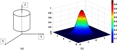
(a) Cylindrical circular vessel model with Gaussian intensity profile at cross section (b).
Eigenvalues and eigenvectors of the Hessian matrix are
| (17) |
| (18) |
that can be generalized to Eqs. (6)–(8) for an ideal tubular structure.
3. Experimental Results and Discussions
3.1. System Setup and Animal Preparation
To demonstrate the feasibility of our segmentation method, we used an OMAG imaging system to acquire the microvasculatural images within tissue beds in vivo, on which the algorithm is tested. The schematic of the OMAG/OCT imaging system is shown in Fig. 2(a), in which we used a superluminescent diode (SLD) with the center wavelength of 1310 nm and bandwidth of 65 nm, delivering an axial resolution of in the air. An optical circulator was used to couple the light from the SLD into fiber-based Michelson interferometer. In the reference arm of the interferometer, a stationary mirror was utilized after polarization controller. In the sample arm of the interferometer, a microscopy objective lens with 18-mm focal length was used to achieve lateral resolution. Then, a optical fiber coupler was utilized to recombine the backscattered light from the sample and the reflected light from the reference mirror. Since the wavelength of the light source is invisible to the human eye, a 633-nm laser diode was used as a guiding beam to locate the imaging position. This reference helps to adjust the sample under the OMAG/OCT system and image the desired location. The recombined light was then routed to a home-built high-speed spectrometer via the optical circulator. The camera in the spectrometer had a line scan rate of . The spectral resolution of the designed spectrometer was that provided a detectable depth range of on each side of the zero-delay line. The measured SNR of the system was with a light power on the sample at .
Fig. 2.

(a) Schematic diagram of the imaging system, where PC represents the polarization controller and CCD is the charged coupled device (camera). (b) Typical mouse ear pinna flattened on the imaging platform. The biopsy punch size is 1 mm. The rectangular box shows typical scanning size of about .
Noninvasive in vivo images were acquired from the pinna of a healthy -weeks-old-male hairless mouse weighing approximately 25 g. During the experiment, the mouse was anesthetized using 2% isoflurance ( , air). The ear was kept flat on a microscope glass using a removable double-sided tape. The experimental protocol was in compliance with federal guidelines for care and handling of small rodents and approved by the Institution Animal Care and Use Committee of the University of Washington, Seattle. Figure 2(b) shows a photograph of a mouse ear pinna taken by a digital camera, in which the area marked by the rectangular box gives a typical field of view and scanning range for OMAG/OCT system, which is in the current setup. In order to scan a larger field on the ear, we used a mechanical translating stage to move the tissue sample to the desired location and after acquisition and processing, the mosaics were stitched together to form a larger image.
The scanning protocol was based on 3-D UHS-OMAG technique.32,33 The x-scanner (fast B-scan) was driven with a saw tooth waveform and the y-scanner (slow C-scan) was driven with a step function waveform. The fast and slow scanners covered a rectangular area of on the sample. Each B-scan consisted of 400 A-lines covering a range of on the sample. The C-scan (3-D scan) consisted of 400 scan locations with a B-scan repetition of 8 frames/location for flow imaging and quantification. The total size of the data set was A-lines. In order to cover a large field of view, multiple 3-D scan were acquired and the sample was translated using a mechanical stage. This allowed imaging an area of on the mouse ear pinna.
After pre-processing of the captured raw data to remove the autocorrelation artifacts,48 the data was then processed off-line using matlab© (MathWorks) which processed repeated B-scans at the same spatial location and generated a cross sectional blood flow perfusion map using ED-based filtering technique.36 Each structure cross section structure frame was processed using the proposed Hessian filter and the lymphatic vessels between stratum corneum and cartilage were segmented. Then, the adjacent cross sections were visualized in a volumetric formation to show 3-D information and vessel map. The main assumption about lymphatic vessels in the OCT structure image is their low scattering property due to the transparency of lymph fluid. Therefore, shadows below vessels, attenuation, and absorption in the ear tissue can influence the segmentation performance. In order to alleviate these problems, we performed shadow removal and contrast enhancement based on Girard et al.49 in the pre-processing step.
Figure 3(a)–3(c) shows blood vessels, lymphatic vessels and structure cross section images of a selected location on the ear, respectively. Figure 3(d)–3(f) shows the volumetric blood vessels and lymphatic vessels map, respectively. The lymphatic vessels are coded by green color and blood flow perfusion is coded with orange. By combining blood flow perfusion and lymphatic vessels from Fig. 3(d) and 3(e), Fig. 3(f) is generated that shows 3-D complications of the circulatory system.
Fig. 3.

Typical cross sectional images of processed blood vessels (a), segmented lymphatic vessels (b) and OCT structure B-mode (c) and their corresponding 3-D volume rendering of blood vessels (d) and lymphatic vessels (e). The cross section location is also marked. (f) Combined blood vessels (orange color) and lymphatic vessels (green color) in volume rendering.
3.2. Application of Imaging Lymph Vessels In Vivo
In general, segmentation and visualization of lymphatic vessels depend on the resolution and quality of captured structure images. The typical size of lymphatic capillaries in a normal mouse ear is and falls below the spatial resolution of our system. However, lymphatic vessels tend to enlarge in response to injury and can be detected with our system. In order to observe the capability of our segmentation method, we created a biopsy punch wound on the mouse ear and monitored the dynamics and healing process of lymphatic and blood vessels around the wound.50 Although no significant lymph was detected on the baseline image due to the limitation of the spatial resolution, immediately after inducing the punch the lymphatic vessels were significantly enlarged around the wound and in the downstream tissue. Figure 4(a)–4(d) shows the process of vasculature remodeling and lymphatic vessel response to the wound. Each image is composed of 9 OCT-OMAG mosaics acquired around the wound area. Blood vessels are orange-coded and lymphatic vessels were color-coded with green. The peak activity of lymphatic vessel enlargement was observed around week after inducing the wound. This observation is in agreement with the wound healing phases during the inflammatory phase.20,51,52 The immediate response of lymphatic vessels after inducing the punch [Fig. 4(a)] was mainly concentrated around the wound, collaterals, and downstream of the injured vessels. However, the size of the lymphatic vessels had significantly increased after 1 week [Fig. 4(b)] and it was not only around the wound, but also at farther locations on the ear. Then, the size and distribution of lymphatic vessels reduced on Day 15 and Day 22 [Fig. 4(c) and 4(d), respectively] and was mainly around the wound area, probably due to inflammation. Wound healing and tissue regeneration are associated with angiogenesis. Angiogenesis can be observed starting on Day 8, where a new capillary network is formed around the wound area in the form of macrophage and eventually matures in the form of new vessels inside the wound.
Fig. 4.

Microvasculature and lymphatic vessel response to a wound induced by biopsy punch. Each image is composed of nine overlapping 3-D OCT scans. The lymphatic vessels are color-coded and overlaid on top of blood vessels (gray-coded) and visualized for every week after the injury. (a) Day 1 corresponds to immediate response after the punch. (b) Day 8, (c) Day 15, (d) Day 22. The lymphatic vessel size was smaller than our system before inducing the punch and no significant lymph vessel was observed.
3.3. Quantification of Vessel Diameter and Vessel Area Density
In order to quantify the lymphatic vessel response to biopsy punch, two parameters were measured.
1-Lymphatic vessel area density (LVAD) was defined as the area of the segmented lymphatic vessels in the projection view divided by the area of the ear given by
| (19) |
2-Lymphatic vessel diameter (LVD) was quantified using Euclidean distance transform (EDT) of the binarized lymphatic vessel en-face projection map.53 The EDT of each pixel in a binary image measures the Euclidean distance between that pixel and the nearest nonzero pixel element of that image. First, the lymphatic vessel map was binarized above a threshold. Then, the vessel centerline was extracted by skeletonizing the binary vessel map. Finally, the distance transform of the intensity-inverted lymphatic vessel map was estimated at each vessel centerline pixel. EDT at the vessel centerline is an estimate of the vessel diameter.
For each imaging time point after inducing the biopsy punch, LVAD, mean value, and standard deviation of LVD were calculated. The measured LVAD and LVD values are given in Table 1 which is congruent with the results of Fig. 4. The lymphatic vessel response was observed immediately after creating the wound. Peak LVAD and LVD were observed on Day 8 and eventually at Day 22 they decreased below values of Day 1.
Table 1.
LVAD and LVD on imaging time points. LVD is given by deviation.
| Day 1 | Day 8 | Day 15 | Day 22 | |
|---|---|---|---|---|
| LVAD | 0.08 | 0.21 | 0.09 | 0.06 |
| LVD |
Note that our main assumption about the lymphatic vessel is that its lumen is of transparency and tubular vessel-like structure. The quality of observed lymphatic vessel lumen on OCT structure image highly depends on the system resolution and speckle noise. This causes estimation errors in the process, limiting the sensitivity of OCT system to pick up small lymphatic vessels. By increasing the system resolution and reducing speckle noise, the system sensitivity to image lymphatic vessels will increase. In this paper, we mainly focused on a segmentation technique that allows for segmentation of such structures. The current OCT setup limits the minimum detectable lymph structures to its spatial resolution. Of course, detecting smaller lymph capillaries requires a higher-resolution OCT system and an approach to efficiently reduce the speckle noise. Hence, the parameters (LVAD and LVD) only provide the quantification of the detectable lymphatic vessels with our system, leading to a biased estimation. We should also note that lymph flow is very irregular and the observed phenomenon regarding enlargement of lymphatic vessels after injury and their remodeling over time, although repeatedly observed in different mice models, came along with some complications that are beyond the scope of this paper. We have repeatedly observed that immediately after inducing a wound on mice ear pinna, some lymphatic vessels that were not obvious in the baseline image enlarged and after a couple of weeks, some enlarged vessels were always present. However, the understanding of remodeling and lymph flow inside these structures requires further research efforts. Again, this study demonstrates the usefulness of proposed method in the study of a skin wound. Although very promising, the detailed study of the microvascular and lymphatic responses to the wound is, however, outside the scope of this study.
3.4. Comparison with Intensity-Threshold Method
In comparison to the intensity-threshold method, Hessian filters are more robust to the noise and intensity variations in the OCT structure image. Also, Hessian filters take the physical appearance of the structure and quantify the closeness to a tubular structure. Figure 5 shows the comparison between the Hessian vesselness filter and the intensity-threshold method. Figure 5(a) and 5(d) shows structure cross sections with visible lymphatic vessels. Figure 5(b) and 5(e) shows lymphatic vessel segmented based on Hessian vesselness filters on the structure images and Fig. 5(c) and 5(f) shows the segmentation results using the intensity threshold on the structure images of Fig. 5(a) and 5(d), respectively. Due to their segmentation nature, the Hessian vesselness method produced smoother vessel lumens and was more sensitive to vessel shape while the intensity-threshold method had no sensitivity to the vessel shape and size (red pointers). It can be observed that the intensity-threshold method is less robust to noise and the threshold parameters and gray-level values at the vessel lumen and can significantly influence the shape of the segmented vessels. Also, the shadows below the blood vessels can produce false alarms (yellow and cyan pointers). Therefore, segmenting lymphatic vessels using intensity-threshold segmentation requires an extra step to manually remove noisy areas while the Hessian-based method can be used as an automated step without the need of manual segmentation.
Fig. 5.
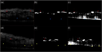
Comparison between the Hessian vesselness filter and the intensity-threshold method. (a and d) OCT structure cross section of mouse ear, (b and e) lymphatic vessels segmented using Hessian vesselness filters and (c and f) corresponding lymphatic vessels segmented using intensity-thresholding method. Blue and yellow arrows indicate the sensitivity of intensity-thresholding method to noise and intensity variations. Red arrows indicate that intensity-thresholding method is not sensitive to vessel shape.
4. Conclusions
In this paper, we propose an automatic filtering technique and vesselness model based on Hessian multi-scale vesselness filters for segmenting lymphatic vessel in OCT structure images. Hessian filters estimate tubular and vessel-like structures and the multi-scale approach allowed segmenting vessels with different sizes. The use of this segmentation technique along with OMAG allows label-free noninvasive, concurrent visualization of blood and lymphatic vessels in vivo. In comparison to the existing method based on intensity threshold, Hessian filters are more robust to the noise and intensity variations in the OCT structure image. Also, Hessian filters take the physical appearance of the structure and quantify the closeness to a tubular structure.
In order to observe the capability of our segmentation method, we created a biopsy punch wound on the mouse ear and monitored the dynamics and healing process of lymphatic and blood vessels around the wound. Although no significant lymph was detected on the baseline image, immediately after inducing the punch, the lymphatic vessels were significantly enlarged around the wound and in the downstream tissue. In order to quantify the lymphatic vessel response to biopsy punch, two parameters were measured: LVAD and LVD. The lymphatic vessel response was observed immediately after creating the wound. Peak LVAD and LVD were observed on Day 8 and eventually at Day 22 they decreased below values of Day 1.
Lymphatic vessels play an important role in cancer, immune system response, inflammatory disease, wound healing, and tissue regeneration. Development of imaging techniques and visualization tools for lymphatic vessels is valuable in understanding the mechanisms and studying therapeutic methods in related disease and tissue response. Up to now, due to the lack of label-free noninvasive imaging techniques, lymphatic vessels have been ignored and their behavior in the disease and their response to treatment methods is not very well understood. Label-free noninvasive imaging and segmentation of lymphatic vessels as proposed here may be useful in different applications such as dermatology, cosmetic and beauty, cancer, wound healing, and infectious diseases that the lymphatic system plays an important role in delivering immune response and draining waste. The observed lymphatic vessels on the structure images are directly related to the resolution of the system. By increasing the system resolution, smaller lymphatic vessels and capillaries could also be observed and eventually segmented using our proposed method.
Acknowledgments
This work was supported in part by research grants from the National Institutes of Health (R01EB009682 and R01HL093140). The funders had no role in study design, data collection and analysis, decision to publish, or preparation of the manuscript.
Appendix: Implementation of 2-D Hessian Vesselness Filters
We briefly describe our implementation approach which is partially taken from open source codes shared on matlab central file exchange center by Marc Schrijver and Drik-Jan Kroon and modified to our specific application.
The Gaussian function at different scales suppresses the noise before using Laplacian on the edges. From linear system theory, we can derive the following equation
| (20) |
and similarly
| (21) |
If the intensity values of the input image are given by where is the spatial location and is the filter scale value, the Hessian matrix can be represented by
| (22) |
where is the Gaussian function at scale given by (for simplicity we omitted the normalizing factor ).
Therefore,
| (23) |
| (24) |
| (25) |
and the eigenvalues of the Hessian matrix can be derived by
| (26) |
and their corresponding eigenvectors are
| (27) |
| (28) |
When implementing on Matlab (The Mathworks) or any programming language, it is not necessary to calculate eigenvalues and eigenvectors at each pixel, and the process can be parallelized by calculating the eigenvalues of the 2-D image matrix using Eq. (26).
Since one of the vesselness parameters () requires division by , the corresponding matrix has to be replaced with a small epsilon value to avoid division by zero. We typically utilized scale values ranging and masked out the segmented vessels with . However, depending on the vessel sizes of interest, these parameters can be modified. Also, the normalization factors of Eq. (14) were experimentally tested to work best when set to and .
References
- 1.Alitalo K., Tammela T., Petrova T. V., “Lymphangiogenesis in development and human disease,” Nature 438(7070), 946–953 (2005). 10.1038/nature04480 [DOI] [PubMed] [Google Scholar]
- 2.Oliver G., “Lymphatic vasculature development,” Nat. Rev. Immunol. 4(1), 35–45 (2004). 10.1038/nri1258 [DOI] [PubMed] [Google Scholar]
- 3.Rockson S. G., “Preface the lymphatic continuum revisited,” Ann. New York Acad. Sci. 1131(1), 9–10 (2008). 10.1196/nyas.2008.1131.issue-1 [DOI] [PubMed] [Google Scholar]
- 4.Kinmonth J. B., “Lymphangiography in man: a method of outlining lymphatic trunks at operation,” Clin. Sci. 11(1), 13–20 (1952). [PubMed] [Google Scholar]
- 5.Partsch H., Urbanek A., Wenzel-Hora B., “The dermal lymphatics in lymphoedema visualized by indirect lymphography,” Br. J. Dermatol. 110(4), 431–438 (1984). 10.1111/bjd.1984.110.issue-4 [DOI] [PubMed] [Google Scholar]
- 6.Suga K. N., et al. , “Visualization of breast lymphatic pathways with an indirect computed tomography lymphography using a nonionic monometric contrast medium iopamidol: preliminary results,” Invest. Radiol. 38(2), 73–84 (2003). 10.1097/00004424-200302000-00002 [DOI] [PubMed] [Google Scholar]
- 7.Yuan Z., et al. , “The role of radionuclide lymphoscintigraphy in extremity lymphedema,” Ann. Nucl. Med. 20(5), 341–344 (2006). 10.1007/BF02987244 [DOI] [PubMed] [Google Scholar]
- 8.McNeill G. C., et al. , “Whole-body lymphangioscintigraphy: preferred method for initial assessment of the peripheral lymphatic system,” Radiology 172(2), 495–502 (1989). [DOI] [PubMed] [Google Scholar]
- 9.Szuba A., et al. , “The third circulation: radionuclide lymphoscintigraphy in the evaluation of lymphedema,” J. Nucl. Med. 44(1), 43–57 (2003). [PubMed] [Google Scholar]
- 10.Lardinois D., et al. , “Staging of non–small-cell lung cancer with integrated positronemission tomography and computed tomography,” New Engl. J. Med. 348(25), 2500–2507 (2003). [DOI] [PubMed] [Google Scholar]
- 11.Clément O., Luciani A., “Imaging the lymphatic system: possibilities and clinical application,” Eur. Radiol. 14(8), 1498–1507 (2004). 10.1007/s00330-004-2265-9 [DOI] [PubMed] [Google Scholar]
- 12.Misselwitz B., “MR contrast agents in lymph node imaging,” Eur. J. Radiol. 58(3), 375–382 (2006). 10.1016/j.ejrad.2005.12.044 [DOI] [PubMed] [Google Scholar]
- 13.Barrett T., Choyke P. L., Kobayashi H., “Imaging of lymphatic system: new horizons,” Contrast Media Molec. Imag. 1(6), 230–245 (2006). 10.1002/(ISSN)1555-4317 [DOI] [PubMed] [Google Scholar]
- 14.Fischer M., et al. , “Flow velocity of cutaneous lymphatic capillaries in patients with primary pymphedema,” Microcirculation 17(3), 143–149 (1997). 10.1159/000179222 [DOI] [PubMed] [Google Scholar]
- 15.Mellor R. H., et al. , “Enhanced cutaneous lymphatic network in the forearms of women with postmastectomy oedema,” J. Vasc. Res. 37(6), 501–512 (2000). 10.1159/000054083 [DOI] [PubMed] [Google Scholar]
- 16.Gurfinkel M., et al. , “Pharmacokinetics of ICG and HPPH-car for the detection of normal and tumor tissue using fluorescence, near-infrared reflectance imaging: a case study,” Photochem. Photobiol. 72(1), 94–102 (2000). [DOI] [PubMed] [Google Scholar]
- 17.Kuznetsov Y. L., Kalchenko V. V., Meglinski I. V., “Multimodal imaging of vascular network and blood microcirculation by optical diagnostic techniques,” Quant. Electron. 41(4), 308–313 (2011). 10.1070/QE2011v041n04ABEH014602 [DOI] [Google Scholar]
- 18.Banerji S., et al. , “LYVE-1, a new homologue of CD44 glycoprotein, is a lymph specific receptor for hyaluronan,” J. Cell Biol. 144(4), 789–801 (1999). 10.1083/jcb.144.4.789 [DOI] [PMC free article] [PubMed] [Google Scholar]
- 19.Tammela T., Alitalo K. “Lymphangiogenesis: molecular mechanisms and future promise,” Cell 140(4), 460–476 (2010). 10.1016/j.cell.2010.01.045 [DOI] [PubMed] [Google Scholar]
- 20.Martínez-Corral I., et al. , “In vivo imaging of lymphatic vessels in development, wound healing, inflammation, and tumor metastasis,” Proc. Natl. Acad. Sci. U.S.A. 109(16), 6223–6228 (2012). 10.1073/pnas.1115542109 [DOI] [PMC free article] [PubMed] [Google Scholar]
- 21.Kalchenko V., et al. , “Label free in vivo laser speckle imaging of blood and lymph vessels,” J. Biomed. Opt. 17(5), 050502 (2012). 10.1117/1.JBO.17.5.050502 [DOI] [PubMed] [Google Scholar]
- 22.Kalchenko V., et al. , “In vivo characterization of tumor and tumor vascular network using multi-modal imaging approach,” J. Biophoton. 4(9), 645–649 (2011). [DOI] [PubMed] [Google Scholar]
- 23.Huang D., et al. , “Optical coherence tomography,” Science (New York) 254(5035), 1178 (1991). 10.1126/science.1957169 [DOI] [PMC free article] [PubMed] [Google Scholar]
- 24.Fercher A. F., et al. , “Optical coherence tomography-principles and applications,” Rep. Prog. Phys. 66(2), 293–303 (2003). 10.1088/0034-4885/66/2/204 [DOI] [Google Scholar]
- 25.Tomlins P. H., Wang R. K., “Theory, developments and applications of optical coherence tomography,” J. Phys. D: Appl. Phys. 38(15), 2519 (2005). 10.1088/0022-3727/38/15/002 [DOI] [Google Scholar]
- 26.Leitgeb R., Hitzenberger C., Fercher A. F., “Performance of Fourier domain vs. time domain optical coherence tomography,” Opt. Exp. 11(8), 889–894 (2003). 10.1364/OE.11.000889 [DOI] [PubMed] [Google Scholar]
- 27.Choma M., et al. , “Sensitivity advantage of swept source and Fourier domain optical coherence tomography,” Opt. Exp. 11(18), 2183–2189 (2003). 10.1364/OE.11.002183 [DOI] [PubMed] [Google Scholar]
- 28.An L., Subhash H. M., Wang R. K., “Full range complex spectral domain optical coherence tomography for volumetric imaging at 47 000 A-scans per second,” J. Opt. 12(8), 84003 (2010). 10.1088/2040-8978/12/8/084003 [DOI] [PMC free article] [PubMed] [Google Scholar]
- 29.Wang R. K., “In vivo full-range complex Fourier domain optical coherence tomography,” Appl. Phys. Lett. 90(5), 054103 (2007). [Google Scholar]
- 30.Wang R. K., et al. , “Three dimensional optical angiography,” Opt. Exp. 15(2), 4083–4097 (2007). 10.1364/OE.15.004083 [DOI] [PubMed] [Google Scholar]
- 31.Wang R. K., Hurst S. “Mapping of cerebrovascular blood perfusion in mice with skin and cranium intact by optical micro-angiography at 1300 nm wavelength,” Opt. Exp. 15 11402–11412 (2007). 10.1364/OE.15.011402 [DOI] [PubMed] [Google Scholar]
- 32.Wang R. K., et al. , “Depth-resolved imaging of capillary networks in retina and choroid using ultrahigh sensitive optical microangiography,” Opt. Lett. 35(9), 1467–1469 (2010). 10.1364/OL.35.001467 [DOI] [PMC free article] [PubMed] [Google Scholar]
- 33.An L., Qin J., Wang R. K., “Ultrahigh sensitive optical microangiography for in vivo imaging of microcirculations within human skin tissue beds,” Opt. Exp. 18(8), 8220–8228 (2010). 10.1364/OE.18.008220 [DOI] [PMC free article] [PubMed] [Google Scholar]
- 34.Wang R. K., “Method and apparatus for ultrahigh sensitive optical microangiography,” WIPO Patent 2011097631 (12 August 2011).
- 35.An L., Shen T. T., Wang R. K., “Using ultrahigh sensitive optical microangiography to achieve comprehensive depth resolved microvasculature mapping for human retina,” J. Biomed. Opt. 16(10), 106013 (2011). 10.1117/1.3642638 [DOI] [PMC free article] [PubMed] [Google Scholar]
- 36.Yousefi S., Zhi Z., Wang R. K., “Eigendecomposition-based clutter filtering technique for optical microangiography,” IEEE Trans. Biomed. Eng. 58(8), 2316–2323 (2011). 10.1109/TBME.2011.2152839 [DOI] [PMC free article] [PubMed] [Google Scholar]
- 37.An L., Shen T. T., Wang R. K., “Using ultrahigh sensitive optical microangiography to achieve comprehensive depth resolved vasculature mapping for human retina,” J. Biomed. Opt. 16(10), 106013 (2011). 10.1117/1.3642638 [DOI] [PMC free article] [PubMed] [Google Scholar]
- 38.Lin A., et al. , “High speed spectral domain optical coherence tomography for retinal imaging at 500,000 A-lines per second,” Biomed. Opt. Exp. 2(10), 2770–2783 (2011) 10.1364/BOE.2.002770 [DOI] [PMC free article] [PubMed] [Google Scholar]
- 39.Jia Y., Li P., Wang R. K., “Optical microangiography provides an ability to monitor responses of cerebral microcirculation to hypoxia and hyperoxia in mice,” J. Biomed. Opt. 16(9), 096019 (2011). 10.1117/1.3625238 [DOI] [PMC free article] [PubMed] [Google Scholar]
- 40.Zhi Z., et al. , “Highly sensitive imaging of renal microcirculation in vivo using ultrahigh sensitive optical microangiography,” Biomed. Opt. Exp. 2(5), 1059–1068 (2011). 10.1364/BOE.2.001059 [DOI] [PMC free article] [PubMed] [Google Scholar]
- 41.Qin J., et al. , “In vivo volumetric imaging of microcirculation within human skin under psoriatic conditions using optical microangiography,” Lasers Surg. Med. 43(2), 122–129 (2011). 10.1002/lsm.v43.2 [DOI] [PMC free article] [PubMed] [Google Scholar]
- 42.Vakoc B., et al. , “Three-dimensional microscopy of the tumor microenvironment in vivo using optical frequency domain imaging,” Nat. Med. 15(10), 1219–1223 (2009). 10.1038/nm.1971 [DOI] [PMC free article] [PubMed] [Google Scholar]
- 43.Jung Y., Zhi Z. W., Wang R. K., “3D optical imaging of microvascular network within intact lymph node in vivo,” J. Biomed. Opt. 15(5), 050101 (2010). 10.1117/1.3505724 [DOI] [PMC free article] [PubMed] [Google Scholar]
- 44.Zhi Z., Jung Y., Wang R. K., “Label-free 3D imaging of microstructure, blood and lymphatic vessels within tissue beds in vivo,” Opt. Lett. 37(5), 812–814 (2012). 10.1364/OL.37.000812 [DOI] [PMC free article] [PubMed] [Google Scholar]
- 45.Frangi A., et al. , “Multiscale vessel enhancement filtering,” in Medical Image Computing and Computer-Assisted Interventation—MICCAI’98, pp. 130–137, Springer Berlin Heidelberg; (1998). [Google Scholar]
- 46.Suri J., et al. , “A review on MR vascular image processing algorithms: acquisition and prefiltering: part I,” IEEE Trans. Inf. Technol. Biomed.: Publ. IEEE Eng. Med. Biol. Soc. 6(4), 324 (2002). 10.1109/TITB.2002.804139 [DOI] [PubMed] [Google Scholar]
- 47.Lesage D., et al. , “A review of 3D vessel lumen segmentation techniques: models, features and extraction schemes,” Med. Image Anal. 13(6), 819–845 (2009). 10.1016/j.media.2009.07.011 [DOI] [PubMed] [Google Scholar]
- 48.Wang R. K., Ma Z., “A practical approach to eliminate autocorrelation artifacts for volume-rate spectral domain optical coherence tomography,” Phys. Med. Biol. 51(12), 3231–3239 (2006) 10.1088/0031-9155/51/12/015 [DOI] [PubMed] [Google Scholar]
- 49.Girard M. J., et al. , “Shadow removal and contrast enhancement in optical coherence tomography images of the human optic nerve head,” Invest. Ophthalmol. Vis. Sci. 52(10), 7738–7748 (2011). 10.1167/iovs.10-6925 [DOI] [PubMed] [Google Scholar]
- 50.Jung Y., et al. , “Tracking dynamic microvascular changes during healing after complete biopsy punch on the mouse pinna using optical microangiography,” PloS One 8(2), e57976 (2013). 10.1371/journal.pone.0057976 [DOI] [PMC free article] [PubMed] [Google Scholar]
- 51.Shaw T. J., Martin P., “Wound repair at a glance,” J. Cell Sci. 122(18), 3209–3213 (2009). 10.1242/jcs.031187 [DOI] [PMC free article] [PubMed] [Google Scholar]
- 52.Baum C. L., Arpey C. J., “Normal cutaneous wound healing: clinical correlation with cellular and molecular events,” Dermatol. Surg. 31(6), 674–686 (2005). 10.1111/j.1524-4725.2005.31612 [DOI] [PubMed] [Google Scholar]
- 53.Gonzalez R., Woods R. E., Eddins S. L., Digital image processing using Matlab, Vol. 2, Gatsmark Publishing, Knoxville: (2009). [Google Scholar]