Thermal conductance and basal metabolic rate are part of a coordinated system for heat transfer regulation

Abstract

Thermal conductance measures the ease with which heat leaves or enters  an organism's body. Although the analysis of this physiological variable in relation to climatic and ecological factors can be traced to studies by Scholander and colleagues, only small advances have occurred ever since. Here, we analyse the relationship between minimal thermal conductance estimated during summer (C_min) and several ecological, climatic and geographical factors for 127 rodent species, in order to identify the exogenous factors that have potentially affected the evolution of thermal conductance. In addition, we evaluate whether there is compensation between C_min and basal metabolic rate (BMR)—in such a way that a scale-invariant ratio between both variables is equal to one—as could be expected from the Scholander–Irving model of heat transfer. Our major findings are (i) annual mean temperature is the best single predictor of mass-independent C_min. (ii) After controlling for the effect of body mass, there is a strong positive correlation between log₁₀ (C_min) and log₁₀ (BMR). Further, the slope of this correlation is close to one, indicating an almost perfect compensation between both physiological variables. (iii) Structural equation modelling indicated that C_min values are adjusted to BMR values and not the other way around. Thus, our results strongly suggest that BMR and thermal conductance integrate a coordinated system for heat regulation in endothermic animals and that summer conductance values are adjusted (in an evolutionary sense) to track changes in BMRs.

1. Introduction

Thermal conductance measures the ease with which heat leaves or enters an organism's body (see the electronic supplementary material, box S1) [1]. Although the analysis of this variable in relation to climatic and ecological factors can be traced to Scholander et al. [2–4] back to the Fifties, only small advances have been made ever since those pioneering works. For instance, according to McNab's recent review [5], very few articles dealing with variability and macrophysiological patterns in thermal conductance have been published over the last three decades.

In comparative studies, minimal thermal conductance (C_min) is considered more informative than thermal conductance because in the former, the external factors that modify heat exchange have been eliminated and also because behaviours affecting thermal conductance have been standardized (electronic supplementary material, box S1) [1]. An interesting point regarding C_min is its relationship with basal metabolic rate (BMR). According to the Scholander–Irving classical model of heat transfer, the critical temperature differential (ΔT_m, °C) between body (T_b, °C) and ambient temperature (T_a, °C) is equal to BMR/C_min (°C); which means that both lower C_min and higher BMR may contribute to an increase in thermoregulatory capacity by allowing heat conservation and heat generation, respectively (see electronic supplementary material, box S1) [1,3]. In line with this, McNab [5] recently pointed out that ‘An appreciable decrease in conductance in some cases appears to compensate for a reduction in the rate of metabolism (p. 19)... [which] emphasize that rate of metabolism and thermal conductance are part of a coordinated system (p. 20)’. However, as far as we know, few empirical tests have been conducted to evaluate this intriguing statement. For instance, compensation in C_min values has been suggested for some rodent species inhabiting xeric habitats [6–8] and also for a few Carnivora species with frugivorous or mixed diets [9].

Within this conceptual framework, the aims of this study were twofold. First, to explore the relationship between C_min and several ecological, climatic, and geographical variables for 127 rodent species, in order to identify the exogenous factors that have potentially affected the evolution of thermal conductance. Second, to explicitly test whether there is compensation between C_min and BMR in such a way that the scale-invariant ratio between log₁₀ (C_min) and log₁₀ (BMR) is equal to one.

2. Material and methods

(a). Database description

We downloaded data on minimal thermal conductance estimated during summer months (C_min), body mass (m_b), BMR and geographical coordinates (together with altitude) for 127 rodent species, compiled by Lovegrove [10] (see the electronic supplementary material, table S1). Methodological details on how these variables were assessed are explained elsewhere [10]. Then, for each data point downloaded, we obtained from WorldClim database (http://www.worldclim.org/) the following climatic variables: annual mean temperature (T_med, in °C), minimum temperature of the coldest month (T_min, in °C), maximum temperature of the warmest month (T_max, in °C), temperature annual range (TAR: difference between maximum temperature of the warmest month and minimum temperature of the coldest month, in °C), temperature seasonality (TS: standard deviation of the mean monthly temperature, in °C), mean monthly temperature range (MMTR: mean of the monthly maximum temperature minus the monthly minimum temperature, in °C), isothermality (IT: the mean monthly temperature range divided by the temperature annual range, thus adimensional), accumulated annual rainfall (rainfall, in mm), rainfall of the driest month (R_min, in mm), rainfall of the wettest month (R_max, in mm) and rainfall seasonality (RS: standard deviation of the mean monthly rainfall, in mm) (see the electronic supplementary material, table S1). These variables were obtained using the free software Diva-Gis (http://www.diva-gis.org/). In addition, a net primary productivity map (based on [11]) was downloaded from Socioeconomic Data and Application Center homepage (http://sedac.ciesin.columbia.edu/es/hanpp.html) and an aridity map (based on [12]) was downloaded from the CGIAR Consortium for Spatial Information homepage (http://csi.cgiar.org/Aridity/). Net primary productivity (NPP, in tons of carbon per 0.25° of latitude cell) and aridity index values (Aridity, adimensional) were then obtained for each site using the software ArcGis v. 10 (see the electronic supplementary material, table S1). Aridity index values were multiplied by (−1) in order to obtain a direct relationship between real aridity and index values; thus, in our scale, values larger than −0.030 represent hyper-arid environments, values between −0.031 and −0.200 represent arid environments, values between −0.201 and −0.500 represent semi-arid environments, values between −0.501 and −0.650 represent dry sub-humid environments and values lower than −0.651 represent humid environments. Finally, we compiled data on rodent food habits from the literature and assigned each species to one of the following dietary categories: herbivorous (H), herbivorous–granivorous (HG), granivorous (G), omnivorous (O) and insectivorous (I) (see the electronic supplementary material, table S1).

(b). Data analysis: exogenous factors affecting C_min

The relationships between C_min and exogenous factors were evaluated through standard least-squares regression techniques, using body mass as a covariate. A log₁₀ transformation was applied to C_min and m_b raw data in order to meet the assumption of normality. In these regression analyses, species food habits were ranked according to their approximate assimilable energy content [13] and included as an ordinal variable (herbivorous: 1, herbivorous–granivorous: 2, granivorous: 3, omnivorous: 4 and insectivorous: 5). We estimated the goodness of fit of the 57 343 possible models without interaction terms—i.e. combination of 16 independent variables but taking just two of the following three variables: T_min, T_max and TAR at a time (because TAR is equal to T_max minus T_min)—and used the Bayesian Information Criterion (BIC) to compare them. Specifically, a model was selected as a ‘good model’ if its BIC value did not differ from the overall best model BIC value (which represents, by definition, the lowest BIC value) in more than 2.3 units [14]. All these analyses were performed using the R package leaps [15].

For models selected as ‘good models’, we evaluated the effect of phylogeny on the relationship between C_min and exogenous factors, using a Bayesian Phylogenetic Mixed Model (Bayesian PMM) [16,17], in addition to Bayesian Model Averaging (BMA) [14]. The phylogenetic tree published by Lovegrove [10] was transformed to a Newick formatted tree using the program TreeSnatcherPlus [18]. Taking this tree as the starting point, we decided to incorporate phylogenetic uncertainty in the calculations using BMA because: (i) branch lengths are not known for this tree, and (ii) there are several soft polytomies associated with (i). In consequence, phylogenetic uncertainty was included by generating 1000 trees in which polytomies were randomly resolved (by transforming all multi-chotomies into a series of dichotomies with one or several branches of length zero) and branch lengths were randomly sampled from a uniform distribution (ranging between 0.01 and the maximum branch length). Inverse-Wishart distributions were used as prior for variances (scale = 2, d.f. = 2) with 350 000 iterations, 150 000 of burn-in and a thinning interval of 20. For each comparative model, the effect of exogenous factors on C_min was calculated through linear mixed models, using body mass as a covariate. Then, to estimate the effect of each exogenous factor on C_min, we calculated the proportion of posterior estimates greater than zero (gt0). In short, gt0 can be viewed as the probability of observing either a positive (if gt0 > 0.5) or negative (if gt0 < 0.5) association between the dependent variable (i.e. C_min) and each exogenous factor. Note that when the dependent variable is not affected by the independent variable, this probability is equal to 0.5 (i.e. the distribution of the regression coefficients is centred on zero). All comparative analyses were performed using the software R, through packages ‘APE’ [19] and ‘bmaMCMCanalysis’ (L. Spangenberg, R. Romero and H. Naya; available upon request). Phylogenetically informed analyses were conducted only for the selected ‘good models’ for practical reasons, i.e. the inability to run the phylogenetic analyses for all the 57 343 models, given the computational costs. Thus, it is possible that phylogenetic ‘good models’ are not among the set of non-phylogenetic ‘good models’ that were considered in the phylogenetic analyses.

(c). Data analysis: relationship between C_min and basal metabolic rate

To evaluate whether there is compensation between C_min and BMR, we first estimated the value of the slope between log₁₀ (C_min) and log₁₀ (BMR) through a standard least-squares regression analysis, using log₁₀ (m_b) as a covariate. Then, we tested whether the value of this slope was statistically different from one, using a two-tailed Student t-test. In addition, an analysis of statistical power was performed in order to determine the level of confidence around the null hypothesis (i.e. slope = 1). On the other hand, given that for the analysed dataset, T_med is the best single predictor of mass-independent BMR [20] and also mass-independent C_min (see results), we used a structural equation modelling approach [21] to compare three causal models: (i) annual mean temperature independently affects BMR and C_min (T_med → log₁₀ BMR, T_med → log₁₀ C_min), (ii) mean annual temperature directly affects BMR and indirectly C_min (T_med → log₁₀ BMR → log₁₀ C_min) and (iii) mean annual temperature directly affects C_min and indirectly BMR (T_med → log₁₀ C_min → log₁₀ BMR). In all these models, body mass (log₁₀ m_b) was included as an exogenous variable affecting both C_min and BMR. We used a maximum-likelihood method to estimate the general fit of each model as well as model parameters. The significance of each model was assessed with χ² statistics, which compare the fit between the observed and predicted elements of the covariance matrix [21]. A significant χ²-value means that the tested model is not supported by the data. All these analyses were performed using the modules ‘Multiple Regression’, ‘Power Analysis’, and ‘Structural Equation Modelling’ of the statistical package STATISTICA v. 8.0.

3. Results

(a). Exogenous factors affecting minimal thermal conductance

Statistical analyses with only one independent variable indicate that annual mean temperature was (by far) the best single predictor of mass-independent C_min (figure 1a and table 1). In line with this, multiple factor analyses indicate that models including annual mean temperature plus annual accumulated rainfall/aridity were the best models to explain variation in mass-independent C_min (table 2; electronic supplementary material, table S2). A third multiple factor model including latitude, in addition to annual mean temperature and annual accumulated rainfall, could also be included in the group of ‘good models’, but its ΔBIC value was close to the limit of 2.3 units (table 2; electronic supplementary material, table S2). Regarding phylogenetic analyses, all independent variables—except latitude—had a significant (p < 0.05) or marginally significant (p < 0.1) effect on mass-independent C_min (table 3).

Figure 1.

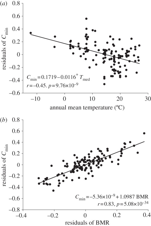
Relationship between (a) residuals of C_min (with regard to body mass) and annual mean temperature and (b) residuals of C_min (with regard to body mass) and residuals of BMR (with regard to body mass). The log₁₀ of BMR, C_min and m_b were used in this analysis.

Table 1.

Parameter estimation (and s.e.) for models including only one exogenous factor in addition to body mass (m_b). BIC, Bayesian Information Criterion value; ΔBIC, BIC model – lowest BIC; r² = proportion of variance explained by the model. The log₁₀ of C_min and m_b were used in these analyses. The probability value associated with each exogenous factor is denoted by asterisks. See material and methods for factors abbreviations.

	intercept		mb		additional variable			BIC	ΔBIC	r2
	B	s.e.	B	s.e.	name	B	s.e.
1	0.74	0.07	0.20	0.04	Tmed***	−0.012	0.002	−79.973	—	0.3322
2	0.97	0.10	0.20	0.04	Tmax***	−0.014	0.003	−75.061	4.912	0.3059
3	0.34	0.08	0.22	0.04	latitude***	0.006	0.001	−71.489	8.484	0.2861
4	0.57	0.06	0.21	0.04	Tmin***	−0.006	0.002	−67.528	12.445	0.2635
5	0.44	0.07	0.22	0.04	aridity***	−0.21	0.05	−67.362	12.611	0.2720
6	0.80	0.10	0.21	0.04	MMTR***	−0.018	0.006	−61.732	18.241	0.2291
7	0.73	0.08	0.21	0.04	IT***	−0.003	0.001	−60.995	18.978	0.2246
8	0.47	0.07	0.21	0.04	TS***	0.00014	0.00005	−58.277	21.696	0.2078
9	0.55	0.07	0.20	0.04	Rmin**	0.0022	0.0009	−56.610	23.363	0.1974
10	0.65	0.08	0.20	0.04	RS**	−0.0012	0.0006	−55.081	24.892	0.1877
11	0.67	0.09	0.19	0.04	diet*	−0.03	0.01	−54.698	25.275	0.1852
12	0.53	0.07	0.20	0.04	rainfall*	−0.00006	0.00003	−54.223	25.750	0.1822
13	0.48	0.09	0.21	0.04	TAR	0.003	0.002	−53.145	26.828	0.1762
14	0.54	0.07	0.20	0.04	Rmax	0.0003	0.0002	−52.538	27.435	0.1712
15	0.54	0.07	0.20	0.04	NPP	9.5×10−8	8.7×10−8	−52.214	27.759	0.1691
16	0.56	0.07	0.20	0.04	altitude	0.000007	0.00003	−51.064	28.909	0.1616

*p < 0.1, **p < 0.05, ***p < 0.01.

Table 2.

Parameter estimation (and s.e.) for the three models selected as ‘good models’ according to the Bayesian Information Criterion (BIC). m_b, body mass; p, number of model parameters; ΔBIC = BIC model – lowest BIC, r², proportion of variance explained by the model. The log₁₀ of C_min and m_b were used in these analyses. See material and methods for exogenous factors abbreviations.

	intercept		mb		Tmed		rainfall		aridity		latitude		BIC	p	ΔBIC	r2
	B	s.e.	B	s.e.	B	s.e.	B	s.e.	B	s.e.	B	s.e.
1	0.71	0.07	0.20	0.03	−0.013	0.002	0.00010	0.00003	—	—	—	—	−87.281	3	—	0.3882
2	0.62	0.07	0.21	0.03	−0.010	0.002	—	—	−0.17	0.04	—	—	−87.280	3	0.001	0.3969
3	0.51	0.14	0.21	0.03	−0.009	0.003	0.00011	0.00003	—	—	0.004	0.002	−85.208	4	2.073	0.3965

Table 3.

Parameter estimation (B), standard deviation (s.d.) and proportion of posterior estimates greater than zero (gt0) for each independent variable included in each selected model (table 2), according to phylogenetically informed analysis. See material and methods for exogenous factors abbreviations. Body mass contribution was highly significant in all cases (gt0 > 0.99).

	Tmed			rainfall			aridity			latitude
	B	s.d.	gt0	B	s.d.	gt0	B	s.d.	gt0	B	s.d.	gt0
1	−0.012	0.004	0.003	7.4×10−5	5.3×10−5	0.92	—	—	—	—	—	—
2	−0.010	0.004	0.01	—	—	—	0.11	0.08	0.90	—	—	—
3	−0.010	0.006	0.08	8.7×10−5	5.7×10−5	0.94	—	—	—	0.003	0.004	0.74

(b). The relationship between C_min and basal metabolic rate

After controlling for the effect of body mass, there was a strong positive correlation between log₁₀ (C_min) and log₁₀ (BMR) (figure 1b). In addition, the slope of this correlation (X ± 1 s.e. = 1.0987 ± 0.0651) was not statistically different from one (t₁₂₄ = 1.51, p > 0.13), indicating an almost perfect compensation between the two energetic variables. However, it is important to note that, with our dataset, the probability of rejecting the null hypothesis (i.e. slope = 1) is larger than 0.80 just for deviation larger than 0.18 from a slope value of one. Finally, results from structural equation modelling indicated that the model where C_min values were adjusted to BMR values (model no. 2) was the only model supported by the data (figure 2).

Figure 2.

Graphical representation of the three causal models evaluated, together with the associated statistics and the partial correlation coefficient for each pathway (±1 s.e.). T_med = annual mean temperature. The log₁₀ of BMR, C_min and m_b were used in this analysis. Total number of observations = 127. p-values were smaller than 0.01 for all partial correlations (except for those between T_med and m_b).

4. Discussion

Global assessment of physiological variables is of paramount relevance in the current scenario of climate change. After all, if we intend to predict how species will respond to accelerated human-caused changes in environmental factors, we need to understand how they respond to these factors in an ecological and evolutionary time frame. Several studies analysing global scale variation in physiological variables have been published in recent years, mainly focusing on metabolic rates [10,13,22–26], metabolic scopes [27,28], thermal tolerance ranges [29–32] and physiological flexibility [33–35]. However, only minor efforts have been made to analyse other relevant physiological variables; such is the case of thermal conductance (but see [10]).

Three results obtained in this study are noteworthy. First, we quantitatively demonstrate that some climatic variables are correlated with thermal conductance. Specifically, single factor statistical models indicate that annual temperature is the best single predictor of mass-independent C_min, while multiple factor statistical models indicate that annual mean temperature plus annual accumulated rainfall/aridity are the major determinants of mass-independent C_min. Interestingly, a recent analysis of 195 rodent species indicates that environmental temperatures (T_med or T_min) plus accumulated rainfall (or NPP) are the main predictors of mass-independent variation in BMR [20]. Thus, it appears that the same exogenous factors are affecting the evolution of both C_min and BMR. Strikingly, our results do not agree with those reported by Lovegrove [10], who found that the coefficient of variation of annual mean rainfall was the only climatic variable correlated with C_min. A potential explanation for this discrepancy is that Lovegrove [10] analysed mass-specific C_min values (i.e. C_min/m_b) instead overall C_min values. To evaluate this possibility, we re-run single factor analyses using C_min/m_b values (data not shown) and found that aridity was the only factor correlated with mass-specific thermal conductance (p < 0.05), which is fairly congruent with Lovegrove's former conclusion. Second, we note that—as could be expected from the Scholander–Irving classical model of heat transfer [3,4]—there is an almost perfect compensation between BMRs and C_min. This result reinforces the idea that the two physiological variables are part of a coordinated system for heat transfer that allows body temperature regulation in endothermic animals [5]. Third, structural equation modelling indicates that annual mean temperature directly affects BMR, and that (summer) C_min values are then adjusted (in an evolutionary sense) to changes in BMR values.

Interestingly, our results are congruent with recent ideas about the evolution of BMR, such as the ‘obligatory heat’ model (OHM) [20,27] and the ‘heat dissipation limit’ theory (HDLT) [36,37]. For instance, it could be possible that colonization of colder environments (e.g. after glacial periods) favoured an increase in BMR through a rise in the size of metabolically expensive organs (as stated by the OHM); but, at the same time, this determined an increase in thermal conductance during the warmer months of the year (as shown here) in order to avoid overheating (as suggested by the HDLT) (figure 3a). In line with this, it is noteworthy that: (i) circumstantial evidence suggests that small tropical and arctic mammals collected during winter appear to be equally well insulated [2,3]; (ii) in contrast with mean and minimum temperatures, maximum temperatures in terrestrial environments change slightly with latitude across the globe [10,29]. In any case, if the scenario described above (and depicted in figure 3a) is correct, a remaining question is why species inhabiting high-latitude environments ‘choose’ to have larger BMR values all year round and increase thermal conductance during summer, instead of (i) maintaining constant BMR and reducing thermal conductance during winter (figure 3b) or (ii) maintaining constant thermal conductance and reducing BMR during summer (figure 3c). Regarding the first alternative, a potential answer is that reducing thermal conductance during winter may represent a costly process that does not result in other benefits than thermal regulation, while maintaining high BMR values—through adjustments in organs size—may represent a costly process that results in several other benefits (e.g. an ability to exploit low-quality diets during winter) in addition to thermal regulation [20]. Another potential explanation for this alternative is that minimum conductance values occurring at low latitudes (i.e. before the colonization of cold habitats) are close to the minimum possible—owing to, for example, an impaired ability to move with a very large fur coat—and thus, a further reduction in thermal conductance is not feasible. With regard to the second alternative, it is fairly clear that a reduction in BMR during summer months—i.e. when food is abundant—may not represent a good strategy, because BMR is positively correlated with reproductive output [5,38,39].

Figure 3.

(a-c) Three hypothetical scenarios for seasonal changes in BMR and C_min (i.e. the slope of the metabolic curves below the thermoneutral zone) in a tropical and a temperate rodent species (see text for a detailed explanation). Note that current data appear to support the scenario depicted in (a). (Online version in colour.)

Finally, two additional points should be noted. First, our analysis is based on interspecific comparisons at a global scale; it does not deny that intraspecific adjustments in BMR can occur [40] but just implies that intraspecific changes are of lower magnitude than interspecific variation in mean values (as it appears to be the case, e.g. compare [20] with [41]). Second, if all the ideas mentioned above are correct, it should be expected that seasonal change in thermal conductance (i.e. a measure of phenotypic flexibility) should increase with latitude, as predicted by the climatic variability hypothesis [40,42].

To end, we care to mention a caveat about the generality of our findings. C_min in small-sized mammals corresponds with the lower limit of thermoneutrality, and hence, C_min values have a clear interpretation from the Scholander–Irving heat transfer model. This may not be the case for intermediate and large animals, in which a circulatory separation between core and shell temperature could determine a reduction in thermal conductance values beyond those observed at the lower limit of thermoneutrality [5,43]. Undoubtedly, more studies analysing physiological diversity in different taxonomic groups and taking into account large geographical and temporal scales are needed to understand and predict human impacts on the Earth's ecosystems [44].

Funding statement

This study was funded by  Agencia Nacional de Investigación e Innovación (Uruguay) to L.S., Comisión Nacional de Investigación Científica y Tecnológica (FONDECYT 1130015, Chile) to F.B. and Programa Iberoamericano de Ciencia y Tecnología para el Desarrollo (CYTED 410RT0406) to D.E.N. and F.B. The authors have no conflict of interest to declare.

References

- 1.McNab BK. 2002. The physiological ecology of vertebrates: a view from energetics. New York, NY: Comstock Publishing Associates [Google Scholar]
- 2.Scholander PF, Walters V, Hock R, Irving L. 1950. Body insulation of some arctic and tropical mammals and birds. Biol. Bull. 99, 225–236 (doi:10.2307/1538740) [DOI] [PubMed] [Google Scholar]
- 3.Scholander PF, Hock R, Walters V, Johnson F, Irving L. 1950. Heat regulation in some artic and tropical mammals and birds. Biol. Bull. 99, 237–258 (doi:10.2307/1538741) [DOI] [PubMed] [Google Scholar]
- 4.Scholander PF, Hock R, Walters V, Irving L. 1950. Adaptation to cold in arctic and tropical mammals and birds in relation to body temperature, insulation, and basal metabolic rate. Biol. Bull. 99, 259–271 (doi:10.2307/1538742) [DOI] [PubMed] [Google Scholar]
- 5.McNab BK. 2012. Extreme measures. Chicago, IL: The University of Chicago Press [Google Scholar]
- 6.McNab BK, Morrison PR. 1963. Body temperature and metabolism in subspecies of Peromyscus from arid and mesic environments. Ecol. Monogr. 33, 63–82 (doi:10.2307/1948477) [Google Scholar]
- 7.Lovegrove BG, Heldmaier G, Knight M. 1991. Seasonal and circadian energetic patterns in an arboreal rodent, Thallomys paedulcus, and a burrow-dwelling rodent, Aethomys namaquensis, from the Kalahari desert. J. Therm. Biol. 16, 199–209 (doi:10.1016/0306-4565(91)90026-X) [Google Scholar]
- 8.Bozinovic F, Lagos JA, Marquet PA. 1999. Geographic energetics of the Andean mouse Abrothrix andinus. J. Mammal. 80, 205–209 (doi:10.2307/1383220) [Google Scholar]
- 9.McNab BK. 1995. Energy expenditure and conservation in frugivorous and mixed-diet carnivorans. J. Mammal. 76, 206–222 (doi:10.2307/1382329) [Google Scholar]
- 10.Lovegrove BG. 2003. The influence of climate on the basal metabolic rate of small mammals: a slow–fast metabolic continuum. J. Comp. Physiol. B 173, 87–112 [DOI] [PubMed] [Google Scholar]
- 11.Imhoff ML, Bounoua L. 2006. Exploring global patterns of net primary production carbon supply and demand using satellite observations and statistical data. J. Geophys. Res. 111, D22S12 (doi:10.1029/2006JD007377) [Google Scholar]
- 12.Trabucco A, Zomer RJ, Bossio DA, van Straaten O, Verchot LV. 2008. Climate change mitigation through afforestation/reforestation: a global analysis of hydrologic impacts with four case studies. Agric. Ecosyst. Environ. 126, 81–97 (doi:10.1016/j.agee.2008.01.015) [Google Scholar]
- 13.Speakman JR. 2000. The cost of living: field metabolic rates of small mammals. In Advances in ecological research (eds Fisher AH, Raffaelli DG.), pp. 178–294 San Diego, CA: Academic Press [Google Scholar]
- 14.Raftery AE, Madigan D, Hoeting JA. 1997. Bayesian model averaging for regression models. J. Am. Stat. Assoc. 92, 179–191 (doi:10.1080/01621459.1997.10473615) [Google Scholar]
- 15.Lumley T, Miller A. 2009. Leaps: regression subset selection. R package version 2.9. See http://CRAN.R-project.org/package=leaps
- 16.Naya H, Gianola D, Romero H, Urioste JI, Musto H. 2006. Inferring parameters shaping amino acid usage in prokaryotic genomes via Bayesian MCMC methods. Mol. Biol. Evol. 23, 203–211 (doi:10.1093/molbev/msj023) [DOI] [PubMed] [Google Scholar]
- 17.Hadfield JD. 2010. MCMC methods for multi-response generalized linear mixed models: the MCMCglmm. J. Stat. Soft. 33, 1–22 [Google Scholar]
- 18.Laubach T, von Haeseler A. 2007. TreeSnatcher: coding trees from images. Bioinformatics 23, 3384–3385 (doi:10.1093/bioinformatics/btm438) [DOI] [PubMed] [Google Scholar]
- 19.Paradis E, Claude J, Strimmer K. 2004. APE: analyses of phylogenetics and evolution in R language. Bioinformatics 20, 289–290 (doi:10.1093/bioinformatics/btg412) [DOI] [PubMed] [Google Scholar]
- 20.Naya DE, Spangenberg L, Naya H, Bozinovic F. 2013. How does evolutionary variation in basal metabolic rates arise? A statistical assessment and a mechanistic model. Evolution 67, 1463–1476 [DOI] [PubMed] [Google Scholar]
- 21.Shipley B. 2004. Cause and correlation in biology. Cambridge, UK: Cambridge University Press [Google Scholar]
- 22.Rezende EL, Bozinovic F, Garland T., Jr 2004. Climatic adaptation and the evolution of basal and maximum rates of metabolism in rodents. Evolution 58, 1361–1374 [DOI] [PubMed] [Google Scholar]
- 23.White RC, Blackburn TM, Martin GR, Butler PJ. 2007. Basal metabolic rate of birds is associated with habitat temperature and precipitation, not primary productivity. Proc. R. Soc. B 274, 287–293 (doi:10.1098/rspb.2006.3727) [DOI] [PMC free article] [PubMed] [Google Scholar]
- 24.Jetz W, Freckleton RP, McKechnie AE. 2008. Environment, migratory tendency, phylogeny and basal metabolic rate in birds. PLoS ONE 3, e3261 (doi:10.1371/journal.pone.0003261) [DOI] [PMC free article] [PubMed] [Google Scholar]
- 25.McNab BK. 2008. An analysis of the factors that influence the level and scaling of mammalian BMR. Comp. Biochem. Physiol. A 151, 5–28 (doi:10.1016/j.cbpa.2008.05.008) [DOI] [PubMed] [Google Scholar]
- 26.McNab BK. 2009. Ecological factors affect the level and scaling of avian BMR. Comp. Biochem. Physiol. A 152, 22–45 (doi:10.1016/j.cbpa.2008.08.021) [DOI] [PubMed] [Google Scholar]
- 27.Naya DE, Spangenberg L, Naya H, Bozinovic F. 2012. Latitudinal pattern in rodent metabolic flexibility. Am. Nat. 179, E172–E179 (doi:10.1086/665646) [DOI] [PubMed] [Google Scholar]
- 28.Naya DE, Bozinovic F. 2012. Metabolic scope of fish increase with species distribution range. Evol. Ecol. Res. 14, 769–777 [Google Scholar]
- 29.Addo-Bediako A, Chown SL, Gaston KJ. 2000. Thermal tolerance, climatic variability and latitude. Proc. R. Soc. Lond. B 267, 739–745 (doi:10.1098/rspb.2000.1065) [DOI] [PMC free article] [PubMed] [Google Scholar]
- 30.Calosi P, Bilton DT, Spicer JI. 2008. Thermal tolerance, acclimatory capacity and vulnerability to global climate change. Biol. Lett. 4, 99–102 (doi:10.1098/rsbl.2007.0408) [DOI] [PMC free article] [PubMed] [Google Scholar]
- 31.Sunday JM, Bates AE, Dulvy NK. 2011. Global analysis of thermal tolerance and latitude in ectotherms. Proc. R. Soc. B 278, 1823–1830 (doi:10.1098/rspb.2010.1295) [DOI] [PMC free article] [PubMed] [Google Scholar]
- 32.Deutsch CA, Tewksbury JJ, Huey RB, Sheldon KS, Ghalambor CK, Haak DC, Martin PR. 2008. Impacts of climate warming on terrestrial ectotherms across latitude. Proc. Natl Acad. Sci. USA 105, 6668–6672 (doi:10.1073/pnas.0709472105) [DOI] [PMC free article] [PubMed] [Google Scholar]
- 33.Naya DE, Bozinovic F, Karasov WH. 2008. Latitudinal trends in digestive flexibility: testing the climatic variability hypothesis with data on the intestinal length of rodents. Am. Nat. 172, E122–E134 (doi:10.1086/590957) [DOI] [PubMed] [Google Scholar]
- 34.Molina-Montenegro MA, Naya DE. 2012. Latitudinal patterns in phenotypic plasticity and fitness-related traits: assessing the climatic variability hypothesis with an invasive plant species. PLoS ONE 7, e47620 (doi:10.1371/journal.pone.0047620) [DOI] [PMC free article] [PubMed] [Google Scholar]
- 35.Aguilar-Kirigin AJ, Naya DE. 2013. Latitudinal patterns in phenotypic plasticity: the case of seasonal flexibility in lizards’ fat body size. Oecologia. (doi:10.1007/s00442-013-2682-z) [DOI] [PubMed] [Google Scholar]
- 36.Speakman JR, Krol E. 2010. Maximal heat dissipation capacity and hyperthermia risk: neglected key factors in the ecology of endotherms. J. Anim. Ecol. 79, 726–746 [DOI] [PubMed] [Google Scholar]
- 37.Speakman JR, Krol E. 2010. The heat dissipation limit theory and evolution of life histories in endotherms—time to dispose of the disposable soma theory? Integr. Comp. Biol. 50, 793–807 (doi:10.1093/icb/icq049) [DOI] [PubMed] [Google Scholar]
- 38.Koteja P. 2000. Energy assimilation, parental care and the evolution of endothermy. Proc. R. Soc. Lond. B 267, 479–484 (doi:10.1098/rspb.2000.1025) [DOI] [PMC free article] [PubMed] [Google Scholar]
- 39.Sadowska J, Gebczynski A, Konarzewski M. 2013. Basal metabolic rate is positively correlated with parental investment in laboratory mice. Proc. R. Soc. B 280, 20122576 (doi:10.1098/rspb.2012.2576) [DOI] [PMC free article] [PubMed] [Google Scholar]
- 40.Stevens GC. 1989. The latitudinal gradient in geographical range: how so many species coexist in the tropics. Am. Nat. 133, 240–256 (doi:10.1086/284913) [Google Scholar]
- 41.McKechnie AE. 2008. Phenotypic flexibility in basal metabolic rate and the changing view of avian physiological diversity: a review. J. Comp. Physiol. 178, 235–247 [DOI] [PubMed] [Google Scholar]
- 42.Janzen DH. 1967. Why mountain passes are higher in the tropics. Am. Nat. 101, 233–249 (doi:10.1086/282487) [Google Scholar]
- 43.McNab BK. 2002. Short-term energy conservation in endotherms in relation to body mass, habits, and environment. J. Therm. Biol. 27, 459–466 (doi:10.1016/S0306-4565(02)00016-5) [Google Scholar]
- 44.Bozinovic F, Calosi P, Spicer JI. 2011. Physiological correlates of geographic range in animals. Annu. Rev. Ecol. Evol. Syst. 42, 155–179 (doi:10.1146/annurev-ecolsys-102710-145055) [Google Scholar]