Noise models and cryo-EM drift correction with a direct-electron camera

Abstract

Blurring due to specimen-holder drift is a common occurrence in cryo-EM images. Cameras employing active-pixel sensors are capable of high frame rates such that a single low-dose exposure can be acquired as a series of frames. In this paper we consider the possibility of tracking and compensating for overall drift in typical single-particle specimens through the analysis of frame sequences. A problem that arises in tracking through cross-correlation of frames obtained with the DE-12 camera from Direct Electron LLC is the presence of “hot-pixel noise”. This random pattern of bright pixels is highly correlated among frames. We show how a model of this noise can be employed to greatly reduce its effects. A filter function is derived that optimizes the tracking of image shifts by cross-correlation, and we demonstrate the tracking of specimen drift in typical cryo-EM specimens.

1. Introduction

Monolithic active-pixel sensors [1–3] allow the construction of sensitive cameras for electron microscopy. In such a sensor, incident high-energy electrons are detected directly within a silicon chip, and the signal representing the deposited charge is read out by CMOS circuitry that can support very high frame rates. The Gatan K-2 camera [4] can acquire images at 400 frames per second, and provides images from single electron counting mode at 40 frames per second. The Direct Electron DE-12 camera can acquire images at 40 frames per second [5]. As individual frames are 12–16 megapixels in size, these cameras provide a flood of data. A very important advantage of acquiring images at high rates is that movements of the specimen can be tracked and compensated. Brilot et al. [6] have exploited high-speed acquisition by the DE-12 camera to track the displacements and rotations of virus particles as imaged in cryo-EM specimens at low doses of 5 e/A² per frame. They were able to do this tracking by comparing individual images with the known structure of the particles. On the basis of improved images from tracking they have obtained a high-resolution structure with a much smaller dataset than usual [7]. Similarly, Bai et al. [8] have obtained a remarkably high-resolution ribosome structure through the statistical processing of information contained in frames acquired with doses of 1 e/Ų.

In principle it should be possible to follow the movements any cryo-EM specimen as long as it contains a consistent “signal” that can be recognized in the individual images. There is enough information in a typical cryo-EM specimen that a relative shift from one micrograph to the next can be tracked even if the micrographs are acquired with a dose of 2 e/Ų or less. Drift of the specimen holder is a recurring problem in cryo-EM image acquisition, and in a typical image-acquisition session much time is spent waiting for the drift rate to fall below a one or a few angstroms per second. Only at these low rates will an image recorded with a typical exposure time of 1–2 s not be blurred by the specimen movement.

To search for displacements due to specimen drift, the standard technique is to compute the cross-correlation or phase-correlation between frames, and evaluate displacements of the correlation peak from the origin. This is implemented in automated microscopy software, for example Leginon [9] and SerialEM [10]. We sought to use cross correlation to track movements in images acquired with the DE-12 camera from Direct Electron LLC. A typical cryo-EM image is shown in Fig. 1A, and a portion of a frame, representing a 2 e/Ų dose, is shown in Fig. 1B. The problem that gave rise to the investigations in this paper is demonstrated in Fig. 1D. The cross-correlation between the first frame and the others shows a very strong, spurious peak at the origin, much larger than the low-amplitude diffuse peak arising from actual image drift. Only when the spurious peak is removed (Fig. 1E) can the true cross-correlation peak be evaluated.

Figure 1.

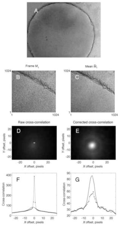
DE-12 images and cross-correlations. A, the sum of 9 frames, each 4k × 3k pixels, corresponding to a total exposure of 18 e/A². B, a 1k × 1k region of the first individual frame M₁₁; C, the corresponding region of the mean of the other frames M̄₂₁. D, unweighted cross-correlation between M₁₁ and M̄₂₁. Note the very bright pixel at zero offset which arises from pixel noise; it is 6 times larger than the true, diffuse peak at centered at the pixel location (−1.6, −3.8). E. The cross-correlation corrected by the subtraction of the estimated pixel-noise spectrum S̃_P. Panels F and G show horizontal slices through the images D and E at a y offset of 0 and −4 pixels, respectively. Solid curves show the raw cross-correlation, and dots indicate the cross-correlation after subtraction of the pixel-noise component. The image is of a cryo-EM specimen of 400 kDa protein particles on a C-Flat grid having 1μm holes, with thin carbon overlaid. Imaging was at 200 keV with 2.0 μm defocus. The image had an effective pixel size of 2.9Å.

The origin of the spurious peak is “pixel noise” arising from trapped charges in individual pixel elements of the detector. The charge decays with a very broad time course ranging from seconds to hours. Figure 2A and B illustrate the pixel noise in a single “dark” raw image from the camera, acquired with no electron beam. Since a dark-image correction is always applied to micrographs, it is more relevant to examine the changes in pixel noise from one image to the next. On a short time scale the difference between two raw dark images is small; the great majority of pixels in the difference image at an interval of 1 second (Fig. 2C and D) show normally-distributed values that reflect the readout noise of the imaging device. This readout noise has a standard deviation of less than 1/10 of the single-electron event size. In addition there is a population of pixels having outlying values, but they comprise only about 1% of the total.

Figure 2.

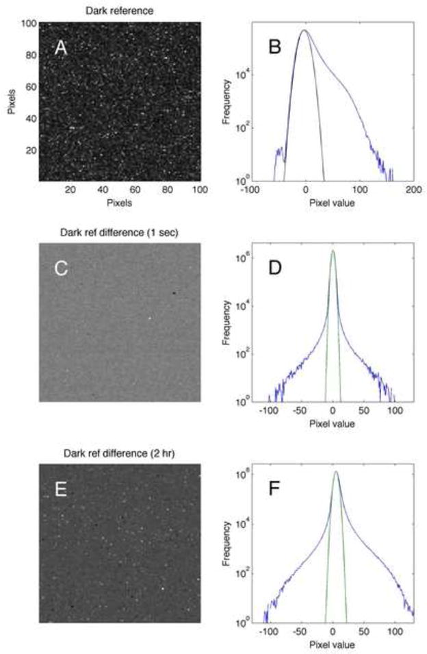
Pixel noise. A, a 100×100 pixel region of a raw dark-reference image, with large-scale trends removed for clarity; B, the corresponding histogram of pixel values. Beyond the narrow Gaussian distribution of pixel values (black curve, S.D. = 7.2 units) there is an excess of “bright” pixels. C, the difference between two dark-reference raw images acquired 1 second apart. D, the corresponding histogram shows small tails (comprising 1% of the pixels) on a Gaussian distribution of pixel values with S.D. = 2.2 (green curve). E, the difference between images acquired 2 hours apart shows many more bright and dark pixels. The tails on the Gaussian distribution (S.D. = 3.2) constitute about 10% of all pixels (area outside the Gaussian curve). The sensitivity of the camera was approximately 30 pixel units per incident electron.

If a comparison is made between two raw images acquired 2 hours apart, the pixel noise is more prominent, presumably due to slow kinetics of recombination of trapped charge in the sensor. The difference (Fig. 2 E and F) has perhaps 10% outlier pixels. The outlier values show a distribution having long tails, with a total spread of ± 100 units, corresponding to the signal from about ± 3 single-electron events. In comparison, a low-dose exposure under our imaging conditions may yield about 4 electrons per pixel in a raw frame. Thus the pixel noise affects a small fraction of the pixels, but it is of considerable magnitude. In this paper we characterize the pixel noise and describe a way in which its effect on cross-correlations can be mitigated.

2. Methods

We acquired low-dose images from cryo-EM specimens using an FEI Tecnai F20 microscope operated at 200 kV. Raw images from the DE-12 camera were stored as 4096 × 3072 pixel TIFF files at a rate of 25 per second. We combined them by summing five images at a time into “frames” to yield an effective rate of 5 per second. The dose rate was 10 e/Ų s, so that each frame represents an electron dose of 2 e/Ų. A typical 1.8 s exposure was thus reduced to a “movie” of 9 frames. The specimen-referred pixel size was 2.9 Å. The data in Fig. 5 consisted of a movie with a very large total accumulated dose. It was obtained by Melody Campbell at the National Resource for Automated Molecular Microscopy under similar conditions except that the pixel size was 1.4 Å and the dose rate was 50 e/Ųs. At this dose rate (2 e/Ų the grouping of images was not necessary for analysis.

Figure 5.

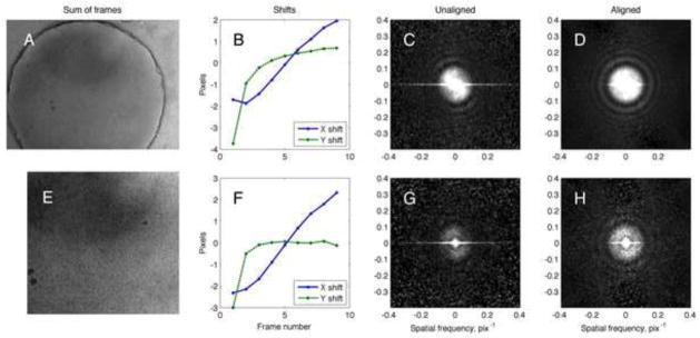
Alignment of a cryo-EM movie of a specimen with thin carbon. A, the final 3k × 4k aligned image M_sum,1 obtained from 9 frames. B, the values of x and y shift that were determined for each frame. C, power spectrum of the summed images without alignment. D, power spectrum of the summed images after alignment. E–H, the same alignment and analysis was applied to a 2k × 2k pixel region in the center of the image. Note that the power spectra of the unaligned images in C and G show “speckles” from the pixel noise which is present in each frame. The speckle phenomenon is suppressed in D and H because, in shifting each frame to align the details of the specimen, the fixed pixel noise is shifted out of register and therefore makes a smaller contribution to the power spectrum.

3. Theory

3.1. Image model

The real-space, i^th frame of a movie is denoted m_0i(x, y), where the subscript zero denotes the absence of corrections for pixel offset and gain. Those corrections are applied through the use of averaged bright and dark images μ_r and ν_r which are taken with a flood beam or no electron beam, respectively. The subscript r enumerates independently-acquired sets of references.

Linear “flat-field” correction of the pixels in a frame is accomplished by pixel-wise operations according to

$$m_{ri}=\frac{m_{0i}-{\nu }_r}{{\mu }_r-{\nu }_r}{k}_{\text{norm}}$$ (1)

where the scalar k_norm is typically set to the mean pixel value of μ_r −ν_r. Noise is introduced in this process mainly through the shot noise in the bright reference image. The reason for acquiring multiple sets of references is to avoid the situation in which common, that is correlated, noise appears in images that are to be cross-correlated. Thus we identify a corrected frame with the subscript indicating which set of references was used.

The specimen being imaged is described by a position-dependent phase shift φ(x, y) of the imaging electrons. In the course of image collection the pattern is translated, operated on by transfer functions, and is corrupted by noise. We denote the Fourier duals of real-space variables by capital letters, so in Fourier space these operations can be represented as pixel-wise products according to

$$M_{ri}=H_S{CT}_{{\mathbf{d}}_i}\mathrm{\Phi }+H_N(N_{\text{shot}}+N_{\text{ref},r})+N_{\text{pix}}$$ (2)

where H_S is the real-valued modulation transfer function of the camera, C is the real-valued phase-contrast transfer function, and T_di is the operator for translation of the image through the vector d_i. Noise is modeled by a white, Gaussian noise field N_shot which is operated on by a modulation transfer function H_N which is distinct from H_S [11]. Also operated on by H_N is the residual shot noise N_ref from the bright reference that was used to correct the image. Finally there is fixed pixel noise N_pix due to the detector itself and which is not filtered by H_N. Because frames are acquired in rapid succession, we assume that the pixel noise is a fixed pattern that is the same in all frames of the movie.

3.2. Cross spectrum and cross-correlation

Tracking the drift in the specimen position is accomplished by estimating changes in the translation vector d between a frame and a template by cross correlation. For frame i we use as a template the mean of all the other frames in the n-frame movie,

$${\overline{M}}_{ri}=\frac{1}{n-1}\sum _{j\ne i}{M}_{rj}$$ (3)

and the corresponding translation operator T̄_i for this mean is given by

$${\overline{T}}_i=\frac{1}{n-1}\sum _{j\ne i}{T}_{{\mathbf{d}}_j}.$$ (4)

The estimated raw cross-spectrum (Fourier transform of the cross-correlation) is computed with distinct references to eliminate any bias from common noise sources,

$$Q_i^0=M_{1i}{\overline{M}}_{2i}^{\ast }.$$ (5)

It is modeled as

$$Q_i^0=H_S^2{C}^2{T}_{{\mathbf{d}}_i}{\overline{T}}_i^{\ast }{\mid \mathrm{\Phi }\mid }^2+S_P+N_Q$$ (6)

where S_P is the power spectrum of the fixed pixel noise, and the zero-mean random variable N_Q represents the noise in the cross spectrum that arises from the various noise terms in (2).

The power spectrum P_i = |M_i|² of an individual frame is similar to that of the cross-spectrum, except that it includes the contributions from shot noise in the image and in the reference:

$$P_i=\left|Q_i^0\right|+H_N^2({\sigma }_{\text{shot}}^2+{\sigma }_{\text{ref}}^2).$$ (7)

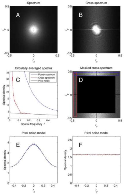
Figure 3 A and B compares the estimated power spectrum and cross-spectrum from a frame. The two functions are similar, but as can be seen in the circularly-averaged quantities in Fig. 3C the power spectrum is much larger in magnitude. At high frequencies the cross-spectrum is comprised almost entirely of pixel noise. The pixel noise, in turn, is a minor part of the total power spectrum, which is dominated by the shot noise.

Figure 3.

Cross spectrum and pixel-noise spectrum. A, the power spectrum of the average image in Fig. 1A. B, the real part of the raw cross-spectrum for the first frame, computed directly as $Q_1^0=M_{11}{\overline{M}}_{21}$ (eqn. 5). C, plots of the circularly-averaged power spectrum, the cross-spectrum, and the estimated pixel noise. The cross-spectrum and the pixel noise spectral density agree very well for frequencies above half the Nyquist frequency, i.e. above 0.25 pixel⁻¹. D, the cross spectrum multiplied by a mask function which preserves the values only for frequencies above 0.4 pixel⁻¹. E, Values of the cross-spectrum in the dashed horizontal box in D, averaged and plotted as a function of f_x. The fitted function (7) is plotted as a black curve. F. Cross-spectrum values averaged over the vertical box in B. The horizontal line is the fitted function.

3.4. Estimating the pixel noise spectrum

A very successful model for the pixel noise of the DE12 camera, as expressed in Fourier space, is

$${\stackrel{\sim }{S}}_P=a_0+a_1{e}^{-f_x^2/2{\sigma }_P^2}$$ (8)

where f_x, the frequency component in the x-direction. We do not know the true physical origin of this noise, but a reasonable explanation is that the trapped charge in each pixel is not a completely independent random quantity; instead roughly 20% of the random charge introduced into each pixel spreads to the horizontally adjacent pixels. The result is a pixel noise spectrum that is not flat in the x-direction, but instead shows a Gaussian peak.

To estimate the parameters of the model, we consider the cross-spectrum (eqn. 6). The factors $H_S^2{C}^2$ in that equation become very small at high frequencies; thus if we define a binary mask (illustrated in Fig. 3D) that excludes the low-frequency components of the measured cross-spectrum $Q_i^0$, we can perform a least-squares fit of (8) to the unmasked region to obtain values for the three parameters a₀, a₁ and σ_P. A representative fit is illustrated in Fig. 3E and F.

Finally given the model for the pixel noise, a corrected cross-correlation is obtained

$$Q_i=Q_i^0-{\stackrel{\sim }{S}}_P.$$ (9)

The fourier transform of this is the quantity displayed in Fig. 1D where it can be seen that the very large, delta-function-like peak has been eliminated by the estimation and subtraction of the model for S_P.

3.3. An optimum filter for cross-correlation

The performance of cross-correlation alignment can be improved through appropriate weighting of the computed cross-spectrum. For example, in some image-alignment problems “phase correlation” is used, where the amplitudes of all Fourier components are forced to unity, and only phase information is used in defining the alignment. We seek to find a function of frequency W for weighting the amplitudes of the cross-spectrum and producing the corresponding weighted cross-correlation,

$$\begin{array}{l}{R}_i={WQ}_i\\ r_i={\mathcal{F}}^{-1}(R_i).\end{array}$$ (10)

An example of a weighting function is a classical matched filter; this maximizes the peak-to-rms noise ratio of the cross-correlation function. However, we wish to maximize the precision of location of the peak. Let us model the cross-correlation of two identical images as the sum of a function r₀ that is symmetric about the origin, and random noise,

$$r(\mathbf{x})=r_0(\mathbf{x})+n_R(\mathbf{x})$$ (11)

as illustrated in Fig. 4A. Suppose the presence of noise causes the peak of the cross-correlation to shift to a position δ away from the origin; thus ∇r(δ) = 0. We also know that at the origin ∇r(0) = δn_R(0). A Taylor expansion of r then yields

Figure 4.

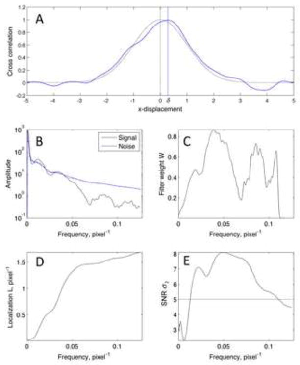
Optimization of cross-correlation for an experimental dataset (the one shown in Fig. 6E–H). A, illustration of a noiseless one-dimensional cross-correlation r₀ (gray curve) and the effect of adding noise (blue curve) which displaces the peak by the distance δ. B, estimates of the cross-spectrum signal, as summed on rings in Fourier space (numerator of eqn. (15)) and the square root of the corresponding noise spectral density (denominator in eqn. (15)). Bumps in the cross-spectrum arise from the contrast transfer function of the imaging process. C, the calculated weighting function W, where values were set to zero beyond f_max = 0.11 pixel⁻¹. D, the calculated localization parameter L (eqn. (14)) as a function of f_max. E, the reliability parameter σ₂ as a function of f_max. It falls below the criterion value of 5 at f_max = 0.11 pixel⁻¹.

$$\delta \approx -\frac{\nabla n_R(0)}{{\nabla }^2{r}_0(0)},$$ (12)

and an estimate for the variance of δ is

$${\stackrel{\sim }{\sigma }}_{\delta }^2=\frac{\langle {|\nabla n_R|}^2\rangle }{{\left({\nabla }^2{r}_0(0)\right)}^2}.$$ (13)

As in Canny’s analysis of line detection [12] let us define a localization parameter $L^2=1/{\stackrel{\sim }{\sigma }}_{\delta }^2$ which is to be maximized through the choice of the weighting function W (eqn. 10). Making use of the Fourier representation of spatial derivatives and writing out explicitly the dependencies on frequency we have

$$L^2=\frac{\left({\displaystyle \sum _{\mathbf{f}}}{f}^{2}Q(\mathbf{f})W(\mathbf{f})\right)}{{\displaystyle \sum _{\mathbf{f}}}{f}^2{|N_Q(\mathbf{f})|}^2{W}^2(\mathbf{f})}$$ (14)

where f=|f| is the magnitude of the spatial frequency, and the sums are take up to a maximum frequency f_max.

Choosing W to be constant along rings of constant frequency ρ_f, we find that L is maximized by the choice

$$W(f)=f\frac{{\displaystyle \sum _{{\rho }_f}}Re\{Q(\mathbf{f})\}}{{\displaystyle \sum _{{\rho }_f}}{|N_Q(\mathbf{f})|}^2},f<f_{max}$$ (15)

With W set to zero at frequencies above some bandwidth f_max to avoid divergence at high frequencies. This function is the same as a matched filter except for the additional factor f which accentuates high-frequency information, helping to sharpen the cross-correlation peak. In practice an average over i of the observed Q_i can serve as the estimate of Q in (15), and a convenient estimate for the noise spectrum is the average of 2Im{Q_i}² because when alignment is exact the imaginary part of Q_i is pure noise. Fig. 4B plots the estimated numerator and denominator of (15) from an actual dataset. Fig. 4C shows the resulting W which has oscillations arising from the contrast-transfer function of the images. Fig. 4D shows the localization parameter as a function of bandwidth.

The approximation in (12) fails when the noise is large, and our approach to this problem is to limit the bandwidth f_max to a value that provides reliable results. At high bandwidth one problem arises with spurious peaks in the cross-correlation when the noise n_R becomes comparable in size to the peak value of the cross-correlation. Another is the possibility of a reversal in sign of the second derivative of the cross correlation; this can occur when the second derivative of the noise ∇²n_R(0) becomes larger in magnitude than the second derivative of the cross-correlation “signal” ∇²r₀(0). In practice a criterion based on this second consideration is more restrictive. We estimate as a reliability parameter the ratio σ₂ of second derivatives, comparing signal amplitude to noise standard deviation,

$${\sigma }_2(f_{max})=\frac{{\displaystyle \sum _{\mid \mathbf{f}\mid <f_{max}}}{f}^{2}W(f){\displaystyle \sum _i}Re\{Q_i(\mathbf{f})\}}{{\left({\displaystyle \sum _{\mid \mathbf{f}\mid <f_{max}}}{f}^2{W}^2(f){\displaystyle \sum _i}2{|Im\{Q_i(\mathbf{f})\left\}\right|}^2\right)}^{1/2}}$$ (16)

and choose the value of f_max at which σ₂ falls to a threshold value of say 5, corresponding to a ratio of 5 standard deviations. Figure 4E shows the dependence of σ₂ on f_max in the representative dataset.

3.4. Tracking specimen movement

The estimation of specimen movement in a frame can be obtained as the displacement vector d_i that maximizes the observed cross-correlation function r_i(d). This is only approximate, however, because r_i as computed from eqns. (5) and (9) represents the translation of frame i relative to the average of all the other frames. In this case it is best to use an iterative process in which a new average is computed after each frame has been translated. When this is done, however, the appropriate translations have to be applied to the correction term S̃_P of eqn. (9) as well. The algorithm can be described as follows.

First set the iteration number k=1 and initialize the displacement vectors ${\mathbf{d}}_i^{(k)}=0$ for all i=1..n. Find the displacement vectors ${\epsilon }_i^{(k)}$ from the peaks of the cross correlations $r_i^{(k)}$ computed as

$$\begin{array}{l}{Q}_i^{(k)}=T_{-{\mathbf{d}}_i^{(k)}}{M}_{1i}\left(\frac{1}{n-1}\sum _{j\ne i}{T}_{-{\mathbf{d}}_j^{(k)}}^{\ast }{M}_{2j}\right)-T_{-{\mathbf{d}}_i^{(k)}}{\overline{T}}_{-{\mathbf{d}}_j^{(k)}}^{\ast }{\stackrel{\sim }{S}}_P\\ r_i^{(k)}(x,y)={\mathcal{F}}^{-1}({WQ}_i^{(k)})\end{array}$$ (17)

Then set ${\mathbf{d}}_i^{(k+1)}={\mathbf{d}}_i^{(k)}+{\epsilon }_i^{(k)}$, update W, and evaluate (17) again to find ${\epsilon }_i^{(k+1)}$. This process is repeated a few times to ensure convergence. The sum of aligned images is finally obtained as

$$M_{\text{sum},\text{r}}=\sum _i{T}_{-{\mathbf{d}}_i}{M}_{ri}.$$ (18)

Results

We implemented a least-squares fitting of the model for pixel noise (eqn. 8) based on cross-spectra computed from the full-size images. Then for the displacement-tracking algorithm (17) the 4096 × 3072 pixel images were first Fourier filtered and downsampled to 1024 × 768 in size, a process that is justified by the fact that high frequency components make little significant contribution to determining the displacement, and interpolation of the cross-correlation peak can be performed to high accuracy as long as the signal is band-limited. All computations were performed in Matlab (MathWorks, Natick MA, USA). Cross-correlations were computed according to eqn. (9) with weights computed from (15) at each iteration.

Figure 5 shows the result of aligning the nine frames of the movie shown Figs. 1 and 3. In this series of frames there was a large, three-pixel initial jump in the y-position between frames 1 and 2 (Fig. 5B), probably due to initial beam-induced specimen movement like that observed by Brilot et al. [6]. In succeeding frames the motion consisted of a gradual displacement in the x direction. When the frames were simply summed the power spectrum (Fig. 5C) shows a substantial loss of information in the x direction, as evidenced by the loss of Thon rings in that direction beyond the first zero, at about 0.1 pixel⁻¹ (0.03 Å⁻¹ at the magnification used). When summed after alignment the resulting image shows Thon rings beyond 0.25 pixel⁻¹ in all directions (Fig. 5D), representing a dramatic improvement in resolution.

The image in Fig. 5A has a strong signal from the thick carbon film that surrounds the hole. Would alignment be possible if only the image in the center of the hole is used, where the only signal arises from protein particles and a thin carbon support film? Fig. 5E-H shows the same analysis performed on a central region that constitutes 1/3 of the image area. Because beam-induced movement might cause different regions of the specimen to show different displacements, the shifts in the whole micrograph and in the central region will not necessarily match. Nevertheless in this case the shifts match within 1 pixel.

How precise are the estimates of shifts? To address this question, we made use of a more recent acquisition series from another cryo-EM specimen, provided to us by Drs. A. Chen and M. Campbell at the National Resource for Automated Molecular Microscopy. This series was acquired with a new backthinned sensor chip and at a higher dose per raw image (2 e/Ų). Recall that in the dataset of Figs. 1, 3 and 5, five raw images were summed to produce each frame of approximately 2 e/Ų dose. The higher dose per raw image in the new series meant that no summation was necessary, and therefore the pixel noise was also not summed. The end result was that the spurious peak in the cross correlation was smaller by about a factor of 5 than in the case shown in Fig. 1. The 52 raw images were separated into two groups of 26 by selecting alternate images. Each movie frame consisted of a single raw image and each of the independent 26-frame movies was analyzed, with results shown in Fig. 6. The entire specimen area included a region of thick carbon in which details are much clearer after alignment (Fig. 6B). The two movies show an rms discrepancy of less than ¼ pixel in both the x and y directions (Fig. 6C and D).

Figure 6.

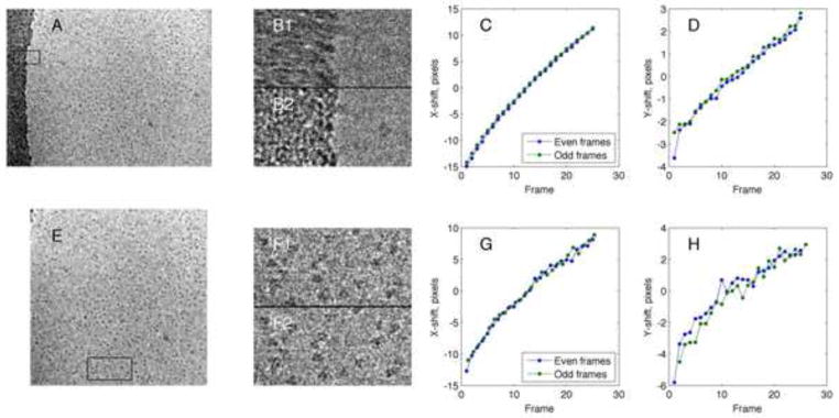
Analysis of a high-dose cryo-EM movie. A series of 52 raw images was acquired from a specimen of influenza hemagglutenin trimers (150 kDa) in ice, imaged at 200 keV with a defocus of 1.6 μm and a pixel size of 1.4Å. Each raw image was obtained with a dose of 2 e/Ų. A, the resulting aligned, summed image stack. B, a closeup of the 512 × 256 pixel region marked by the box in A, shown as sums without (B1) and with (B2) alignment. C, Computed x-displacements in two independent 26-frame “movies” consisting of the odd and even raw images. The position between corresponding frames of the movies showed an rms variation of 0.21 pixels. D, the corresponding y-displacements. Not counting the first pair of frames, the rms variation between the movies was 0.22 pixels. E, the summed image stack from a 3072 × 3072 pixel region that does not include the carbon region in A. F, comparison of unaligned and aligned image sums from a 768 × 384 pixel region (box in E). G and H, the tracked displacements in the independent movies showed rms variations of 0.68 and 0.58 pixel in x and y, respectively. These values correspond well to the localization error of 1.5 pixel⁻¹ predicted for this dataset (Fig. 4D).

The tracking of shifts was then repeated after the frames were cropped to remove the carbon region, leaving only single particles in ice (Fig. 6E). Because of the smaller signal in the cropped images, the rms discrepancy between the two independent movies increased to about 0.6 pixel (Fig. 6G and H) which would correspond to an rms error of 0.4 pixel from the true position in each of the independent movies. The signal in this set of cropped images of single particles in ice, with a dose of 2 e per frame and a specimen area of 0.45 μm on a side, appears to be close to the limit of reliable tracking by cross-correlation. However, summing sets of 2–4 of raw images to produce higher-dose frames, or smoothing the estimated time course of displacements, can readily decrease the tracking error to below ¼ pixel.

5. Discussion

Image blurring due to specimen-holder drift is a common occurrence in cryo-EM studies, and the advent of cameras that provide high-speed acquisition now provides an opportunity for this drift to be tracked and compensated. Brilot et al. [6] have shown that both the position and orientation of single virus particles can be tracked to high precision from cryo-EM images obtained with 5 e/Å exposures. The situation is more difficult in arbitrary cryo-EM specimens where a precise model for the imaged objects is not available; in that case, tracking must make use of the direct comparison of pairs of noisy images.

In this paper we examine this possibility, and find that one problem in comparing noisy images is the fixed-pattern noise due to “hot pixels” in the sensor chip. The effect of this noise is particularly large when the dose per raw image is small. Using a model for this noise, we are able to reduce its influence on specimen tracking by cross-correlation. We also derive an optimized filter for weighting the Fourier components of the cross-correlation function. We find that the effects of specimen-holder drift can be compensated readily when cryo-EM images contain a region of the carbon support film, as in Fig. 5A and 6A. The drift compensation can also be carried out images containing only protein particles suspended in ice (Fig. 5E, 6E) although it is not as precise.

Highlights.

• Active-pixel cameras allow high-frame-rate recording of TEM images.

• We investigate the use of multi-frame exposures to track and compensate for cryo-EM specimen drift.

• Once electronic “hot-pixel” noise is characterized, cross-correlation allows tracking of drift in cryo-EM specimens at low dose.

• We derive a Fourier-space filter that optimizes the tracking of image shifts by cross-correlation.

Abbreviations

CMOS

Complementary metal-oxide-semiconductor

Cryo-EM

Electron cryomicroscopy

References

- 1.Faruqi AR, McMullan G. Electronic detectors for electron microscopy. Q Rev Biophys. 2011;44:357–390. doi: 10.1017/S0033583511000035. [DOI] [PubMed] [Google Scholar]
- 2.Turchetta R, Berst JD, Casadei B, Claus G, Colledani C, Dulinski W, Hu Y, Husson D, Le Normand JP, Riester JL, Deptuch G, Goerlach U, Higueret S, Winter M. A monolithic active pixel sensor for charged particle tracking and imaging using standard VLSI CMOS technology. Nuclear Instruments & Methods in Physics Research Section a-Accelerators Spectrometers Detectors and Associated Equipment. 2001;458:677–689. [Google Scholar]
- 3.Jin L, Milazzo AC, Kleinfelder S, Li S, Leblanc P, Duttweiler F, Bouwer JC, Peltier ST, Ellisman MH, Xuong NH. Applications of direct detection device in transmission electron microscopy. Journal of Structural Biology. 2008;161:352–358. doi: 10.1016/j.jsb.2007.10.007. [DOI] [PMC free article] [PubMed] [Google Scholar]
- 4.Mooney P, Contarato D, Denes P, Gubbens A, Lee B, Lent M, Agard D. A High-Speed Electron-Counting Direct Detection Camera for TEM. Microscopy and Microanalysis. 2011;17:1004–1005. [Google Scholar]
- 5.Bammes BE, Rochat RH, Jakana J, Chen DH, Chiu W. Direct electron detection yields cryo-EM reconstructions at resolutions beyond 3/4 Nyquist frequency. Journal of Structural Biology. 2012;177:589–601. doi: 10.1016/j.jsb.2012.01.008. [DOI] [PMC free article] [PubMed] [Google Scholar]
- 6.Brilot AF, Chen JZ, Cheng A, Pan J, Harrison SC, Potter CS, Carragher B, Henderson R, Grigorieff N. Beam-induced motion of vitrified specimen on holey carbon film. Journal of Structural Biology. 2012;177:630–637. doi: 10.1016/j.jsb.2012.02.003. [DOI] [PMC free article] [PubMed] [Google Scholar]
- 7.Campbell MG, Cheng A, Brilot AF, Moeller A, Lyumkis D, Veesler D, Pan J, Harrison SC, Potter CS, Carragher B, Grigorieff N. Movies of ice-embedded particles enhance resolution in electron cryo-microscopy. Structure. 2012;20:1823–1828. doi: 10.1016/j.str.2012.08.026. [DOI] [PMC free article] [PubMed] [Google Scholar]
- 8.Bai XC, Fernandez IS, McMullan G, Scheres SH. Ribosome structures to near-atomic resolution from thirty thousand cryo-EM particles. eLife. 2013;2:e00461. doi: 10.7554/eLife.00461. [DOI] [PMC free article] [PubMed] [Google Scholar]
- 9.Suloway C, Pulokas J, Fellmann D, Cheng A, Guerra F, Quispe J, Stagg S, Potter CS, Carragher B. Automated molecular microscopy: the new Leginon system. Journal of Structural Biology. 2005;151:41–60. doi: 10.1016/j.jsb.2005.03.010. [DOI] [PubMed] [Google Scholar]
- 10.Mastronarde DN. Automated electron microscope tomography using robust prediction of specimen movements. Journal of Structural Biology. 2005;152:36–51. doi: 10.1016/j.jsb.2005.07.007. [DOI] [PubMed] [Google Scholar]
- 11.Kirkland A. The effects of electron and photon scattering on signal and noise transfer properties of scintillators in CCD cameras used for electron detection. Ultramicroscopy. 1998 [Google Scholar]
- 12.Canny J. A computational approach to edge detection. IEEE Trans Pattern Analysis and Machine Intelligence. 1986;8:679–698. [PubMed] [Google Scholar]