Megavoltage CT imaging quality improvement on TomoTherapy via tensor framelet

Abstract

Purpose: This work is to investigate the feasibility of improving megavoltage imaging quality for TomoTherapy using a novel reconstruction technique based on tensor framelet, with either full-view or partial-view data.

Methods: The reconstruction problem is formulated as a least-square L1-type optimization problem, with the tensor framelet for the image regularization, which is a generalization of L1, total variation, and wavelet. The high-order derivatives of the image are simultaneously regularized in L1 norm at multilevel along the x, y, and z directions. This convex formulation is efficiently solved using the Split Bregman method. In addition, a GPU-based parallel algorithm was developed to accelerate image reconstruction. The new method was compared with the filtered backprojection and the total variation based method in both phantom and patient studies with full or partial projection views.

Results: The tensor framelet based method improved the image quality from the filtered backprojection and the total variation based method. The new method was robust when only 25% of the projection views were used. It required ∼2 min for the GPU-based solver to reconstruct a 40-slice 1 mm-resolution 350 × 350 3D image with 200 projection views per slice and 528 detection pixels per view.

Conclusions: The authors have developed a GPU-based tensor framelet reconstruction method with improved image quality for the megavoltage CT imaging on TomoTherapy with full or undersampled projection views. In particular, the phantom and patient studies suggest that the imaging quality enhancement via tensor framelet method is prominent for the low-dose imaging on TomoTherapy with up to a 75% projection view reduction.

INTRODUCTION

Intensity modulated radiation therapy (IMRT), capable of delivering highly conformal dose to the tumor while sparing the adjacent normal structures, has become the standard treatment for head-and-neck (H&N) and prostate cancer.^{1, 2} The rapid dose falloff delivered by most IMRT plans requires reproducible patient positioning to provide accurate treatment delivery.

The TomoTherapy Hi-Art Helical Radiotherapy System (Accuray, Sunnyvale, CA) is an integrated unit dedicated to IMRT and uses megavoltage CT (MVCT) for volumetric image guidance.^{3, 4, 5} The MVCT images appear noisier than traditional cone beam CT (CBCT) images due, in part to the less efficient detection of megavoltage x rays relative to kilovoltage x rays. The MVCT dose is relatively small, but its daily use raises concerns regarding the total imaging dose.^{6, 7, 8} Improving MVCT image quality for regular or low-dose MVCT scan would improve the utility of the TomoTherapy imaging system.⁹

Inspired by compressive sensing,^{10, 11} a recent technique that has been employed for low-dose image reconstruction is the iterative reconstruction method using the L1-type image regularization, such as total variation (TV).^{12, 13, 14, 15, 16, 17, 18} In our recent work on 4D CBCT,¹⁹ we proposed the tensor framelet (TF), which is better than the framelet for high-dimensional large-scale image reconstruction in terms of its significantly reduced demand on the memory and computational cost.

In this work, using TF, we aim to develop a new reconstruction method to further improve TomoTherapy MVCT imaging quality from the popular filtered backprojection (FBP). We will also compare the TF based reconstruction method with the state-of-art TV based reconstruction method, with both full-view and partial-view (low-dose) data. The low-dose imaging can be achieved through the reduction of either dose intensity or the number of projection views. This study focuses on the latter, and the reconstruction with reduced dose intensity will be studied in the future.

METHODS

Least-square formulation

With the traditional FBP, the 3D CT images on TomoTherapy could be reconstructed slice by slice along the longitudinal direction based on the fan-beam geometry with curved detectors. To utilize the prior that the CT image or its derivates can be smooth and sparse for both the inplane directions and the longitudinal direction, we formulate the image reconstruction as the following iterative least-square minimization problem, in which all slices are reconstructed simultaneously so that the image smoothness and sparsity along the longitudinal direction can be enforced,

$$X=\underset{X}{\arg \min }\frac{1}{2}{\Vert AX-Y\Vert }_2^2+\lambda R\left(X\right).$$ (1)

In Eq. 1, the first term is the L2-norm data fidelity term with the imaging data Y and the 3D image X to be reconstructed, and the second term is the L1-norm image regularization term with the regularization parameter λ and the proper sparsifying transform, which will be discussed next.

Here, A is a linear operator on X that corresponds to the x-ray transform on X slice by slice. Considering the computational efficiency, we use our recently developed new parallel algorithm with O(1) per parallel thread.^{20, 21} On the other hand, similar to the backprojection, we use the GPU-based pixel-driven algorithm for the transpose of A, i.e., the adjoint x-ray transform A^T. That is, the ray passing the center of the pixel is traced back to the detector array for the backprojection value through linear interpolation weighted by the ray intersection length with the pixel.

Tensor framelet

A popular sparsifying transform is the TV.²² For a 3D image X = {x_ijk, i ≤ N_x, j ≤ N_y, k ≤ N_z}, the TV transform is

$$\begin{array}{c}\hfill {\left.DX\right|}_{ijk}={\left.\left[\begin{array}{c}{D}_{x}X\\ D_{y}X\\ D_{z}X\end{array}\right]\right|}_{ijk}=\left[\begin{array}{c}{X}_{i+1,j,k}-X_{ijk}\\ X_{i,j+1,k}-X_{ijk}\\ X_{i,j,k+1}-X_{ijk}\end{array}\right]\end{array}$$ (2)

and the isotropic TV norm is defined as

$$\begin{array}{c}\hfill {R\left(X\right)=\Vert DX\Vert }_1=\sum _{i,j,k}\sqrt{|D_x{X|}^2+|D_y{X|}^2+{\left|D_{z}X\right|}^2}.\end{array}$$ (3)

On the other hand, the combination of the L1 norm and TV was suggested,²³ i.e.,

$$\begin{array}{c}\hfill R\left(X\right)={\Vert X\Vert }_1+{\lambda }_1{\Vert DX\Vert }_1.\end{array}$$ (4)

In this work, we use the TF,^{19, 24} denoted by W, to promote the image smoothness and sparsity, which is a natural multiscale generalization of Eq. 4 with W^TW = I. In particular, we use the TF based 1D piecewise-linear B-spline framelet²⁵ (Fig. 1).

Figure 1.

TF transform. In this example, based on 1D piecewise-linear B-spline framelet, the TF transform of the 3D image consists of the averaged image (D0), the first-order derivative image (D1), the second-order derivative image (D2) at the fine level (L1) and the coarse level (L0) along x-, y-, and z-direction, respectively.

For simplicity, let us first consider a one-level TF. That is, we define the averaging operator

$$\begin{array}{ccc}\hfill {\left.D_{0}X\right|}_{ijk}& =& {\left.\left[\begin{array}{c}{D}_{0x}X\\ D_{0y}X\\ D_{0z}X\end{array}\right]\right|}_{ijk}\hfill \\ & =& \frac{1}{4}\left[\begin{array}{c}{X}_{i+1,j,k}+2X_{ijk}+X_{i-1,j,k}\\ X_{i,j+1,k}+2X_{ijk}+X_{i,j-1,k}\\ X_{i,j,k+1}+2X_{ijk}+X_{i,j,k-1}\end{array}\right],\hfill \end{array}$$ (5)

the first-order derivative operator

$$\begin{array}{c}\hfill {\left.D_{1}X\right|}_{ijk}={\left.\left[\begin{array}{c}{D}_{1x}X\\ D_{1y}X\\ D_{1z}X\end{array}\right]\right|}_{ijk}=\frac{\sqrt{2}}{4}\left[\begin{array}{c}{X}_{i+1,j,k}-X_{i-1,j,k}\\ X_{i,j+1,k}-X_{i,j-1,k}\\ X_{i,j,k+1}-X_{i,j,k-1}\end{array}\right],\end{array}$$ (6)

and the second-order derivative operator

$$\begin{array}{ccc}\hfill {\left.D_{2}X\right|}_{ijk}& =& {\left.\left[\begin{array}{c}{D}_{2x}X\\ D_{2y}X\\ D_{2z}X\end{array}\right]\right|}_{ijk}\hfill \\ & =& \frac{1}{4}\left[\begin{array}{c}-X_{i+1,j,k}+2X_{ijk}-X_{i-1,j,k}\\ -X_{i,j+1,k}+2X_{ijk}-X_{i,j-1,k}\\ -X_{i,j,k+1}+2X_{ijk}-X_{i,j,k-1}\end{array}\right].\hfill \end{array}$$ (7)

Then the TF transform is

$$\begin{array}{c}\hfill WX=\frac{1}{\sqrt{3}}\left[\begin{array}{c}{D}_{0}X\\ D_{1}X\\ D_{2}X\end{array}\right],\end{array}$$ (8)

and similar to isotropic TV norm 3, the TF norm is defined as

$$\begin{array}{c}\hfill {\Vert WX\Vert }_1=\frac{1}{\sqrt{3}}({\lambda }_0\Vert D_0{X\Vert }_1+{\lambda }_1\Vert D_1{X\Vert }_1+{\lambda }_2\Vert D_{2}X{\Vert }_1)\end{array}$$ (9)

with

$$\begin{array}{ccc}\hfill \Vert D_m{X\Vert }_1& =& \sum _{i,j,k}\sqrt{|D_{mx}{X|}^2+|D_{my}{X|}^2+{\left|D_{mz}X\right|}^2},\hfill \\ \hfill m& =& 0,1,2.\hfill \end{array}$$ (10)

On the other hand, as a consequence of Eq. 8, the adjoint TF transform W^T is

$$\begin{array}{c}\hfill W^T\left(WX\right)=\frac{1}{3}\left[D_0^T\left(D_{0}X\right)+D_1^T\left(D_{1}X\right)+D_2^T\left(D_{2}X\right)\right],\end{array}$$ (11)

where

$$\begin{array}{ccc}\hfill D_m^T\left(D_{m}X\right)& =& D_{mx}^T\left(D_{mx}X\right)+D_{my}^T\left(D_{my}X\right)+D_{mz}^T\left(D_{mz}X\right),\hfill \\ \hfill m& =& 0,1,2\hfill \end{array}$$ (12)

with D^T that can be used in the similar fashion with the transpose of TV, i.e., in terms of the pointwise operations instead of forming the matrix D^T explicitly. Therefore, TF generalizes L1 and TV with high-order derivatives.

On the other hand, notice that Eq. 8 can be rewritten as

$$\begin{array}{c}\hfill WX=\frac{1}{\sqrt{3}}\left[\begin{array}{c}{w}_{x}X\\ w_{y}X\\ w_{z}X\end{array}\right],\end{array}$$ (13)

and Eq. 11 can be rewritten as

$$\begin{array}{c}\hfill W^T\left(WX\right)=\frac{1}{3}\left[w_x^T\left(w_{x}X\right)+w_y^T\left(w_{y}X\right)+w_z^T\left(w_{z}X\right)\right],\end{array}$$ (14)

with 1D piecewise-linear B-spline framelet w_x, w_y, w_z and their adjoints. For example,

$$\begin{array}{ccc}\hfill {\left.w_{x}X\right|}_{ijk}& =& {\left.\left[\begin{array}{c}{d}_{0x}X\\ d_{1x}X\\ d_{2x}X\end{array}\right]\right|}_{ijk}\hfill \\ & =& \frac{1}{4}\left[\begin{array}{c}{X}_{i+1,j,k}+2X_{ijk}+X_{i-1,j,k}\\ \sqrt{2}(X_{i+1,j,k}-X_{i-1,j,k})\\ -X_{i+1,j,k}+2X_{ijk}-X_{i-1,j,k}\end{array}\right].\hfill \end{array}$$ (15)

Thus, since w^Tw = I, W^TW = I.

Next, we formulate TF at multilevel based on the 1D framelet operator w. Considering the 1D framelet transform up to L levels (larger number for coarser resolution), we start from the 1D refinement masks for w at level 0 ≤ l ≤ L

$$\begin{array}{c}\hfill h^l=\left[\begin{array}{c}{h}_0^l\\ h_1^l\\ h_2^l\end{array}\right]=\frac{1}{4}\left[\begin{array}{ccccc}1& \underset{2^l-1}{\underbrace{\begin{array}{ccc}0& \cdots & 0\end{array}}}& 2& \underset{2^l-1}{\underbrace{\begin{array}{ccc}0& \cdots & 0\end{array}}}& 1\\ \sqrt{2}& \underset{2^l-1}{\underbrace{\begin{array}{ccc}0& \cdots & 0\end{array}}}& 0& \underset{2^l-1}{\underbrace{\begin{array}{ccc}0& \cdots & 0\end{array}}}& -\sqrt{2}\\ -1& \underset{2^l-1}{\underbrace{\begin{array}{ccc}0& \cdots & 0\end{array}}}& 2& \underset{2^l-1}{\underbrace{\begin{array}{ccc}0& \cdots & 0\end{array}}}& -1\end{array}\right].\end{array}$$ (16)

Then 1D framelet transform w of x is

$$\begin{array}{c}\hfill wx=\left[\underset{\mathrm{Level}:0}{\underbrace{\begin{array}{cc}{d}_1^0{x}^0& d_2^0{x}^0\end{array}}}\cdots \underset{\mathrm{Level}:l}{\underbrace{\begin{array}{cc}{d}_1^l{x}^l& d_2^l{x}^l\end{array}}}\cdots \underset{\mathrm{Level}:L}{\underbrace{\begin{array}{ccc}{x}^{L+1}& d_1^L{x}^L& d_2^L{x}^L\end{array}}}\right],\end{array}$$ (17)

and its transpose w^T is

$$\begin{array}{c}\hfill w^T\left(wx\right)=\sum _{m=1}^2\sum _{l=0}^L{d}_m^l{x}^l+x^{L+1},\end{array}$$ (18)

where

$$\begin{array}{c}\hfill d_m^l{x}^l=h_m^l*x^l\mathrm{and}{x}^{l+1}=d_0^l{x}^l\end{array}$$ (19)

with * for convolution, x⁰ = x, 0 ≤ m ≤ 2, and 0 ≤ l ≤ L.

Based on Eqs. 17, 18, the TF with multilevel is

$$\begin{array}{c}\hfill WX=\frac{1}{\sqrt{3}}\left[\begin{array}{c}{w}_x{X}_x\\ w_y{X}_y\\ w_z{X}_z\end{array}\right],\end{array}$$ (20)

and the adjoint TF with multilevel is

$$\begin{array}{ccc}\hfill W^T\left(WX\right)& =& \frac{1}{3}[\sum _{j,k}{w}_x^T\left(w_x{X}_x^{jk}\right)+\sum _{i,k}{w}_y^T\left(w_y{X}_y^{ik}\right)\hfill \\ & & +\sum _{i,j}{w}_z^T\left(w_z{X}_z^{ij}\right)],\hfill \end{array}$$ (21)

where X_x, X_y, X_z are the unfolded matrices of X along x, y, z dimension, respectively, and the 1D framelet operator w and w^T are with respect to the 1D unfolded dimension x, y, z, respectively. For example, w_xX_x performs 1D framelet transform along each x-line for all combination of y- and z-variables.

Finally, the isotropic TF norm at multilevel is defined as

$$\begin{array}{c}\hfill {\Vert WX\Vert }_1=\frac{1}{\sqrt{3}}\left(\sum _{m=1}^2\sum _{l=0}^L{\lambda }_m^l{\Vert D_m^l{X}^l\Vert }_1+{\lambda }_0^{L+1}{\Vert X^{L+1}\Vert }_1\right),\end{array}$$ (22)

with

$$\begin{array}{ccc}\hfill \Vert D_m^l{X}^l{\Vert }_1& =& \sum _{i,j,k}\sqrt{|D_{mx}^l{X}_x^l{|}^2+|D_{my}^l{X}_y^l{|}^2+{\left|D_{mz}^l{X}_z^l\right|}^2},\hfill \\ \hfill m=1,2\end{array}$$ (23)

and

$$\begin{array}{c}\hfill \Vert X^{L+1}{\Vert }_1=\sum _{i,j,k}\sqrt{|X_x^{L+1}{|}^2+|X_y^{L+1}{|}^2+{\left|X_z^{L+1}\right|}^2}.\end{array}$$ (24)

Notice that the wavelet bases are orthonormal, while the TF bases are redundant. For example, the Haar wavelet includes the low-passed average and the first-order derivatives, while the piecewise-linear TF here also contains the second-order derivatives. In this sense, TF generalizes TV and the wavelet with high-order derivatives for characterizing the smoothness and the sparsity.

On the other hand, TF is more suitable than the standard framelet for the high-dimensional problem in terms of computational efficiency. Take piecewise-linear B-spline framelet, for example. In terms of the memory, the standard framelet requires ∼3^dN memory, while TF requires ∼3dN memory, where d is the number of dimension and N = N_x·N_y·N_z. In terms of the computation cost, the standard framelet needs ∼3^2dN operations, while TF needs ∼3d²N operations. In general, based on n refinement masks in 1D, TF requires ∼ndN memory and ∼nd²N operations, while the standard d-dimensional framelet requires ∼n^dN memory and ∼n^2dN operations.

Split Bregman method

With TF, the formulation is a L1-norm-regularized least-square optimization

$$\begin{array}{c}\hfill X=\underset{X}{\arg \min }\frac{1}{2}{\Vert AX-Y\Vert }_2^2+\lambda {\Vert WX\Vert }_1.\end{array}$$ (25)

Here, we choose the Split Bregman method²⁶ for solving this convex L1-type problem. The method was also used in our prior related work on CT.^{17, 19, 27}

Note that for many algorithms it is required to dynamically reduce the regularization parameter λ during iterations in Eq. 25 for the optimized image quality. However, the problem may become ill-conditioned for a small λ so that the optimal solution may not be reachable.

In comparison, the Split Bregman method works with a fixed and sufficiently large λ. The method goes as follows. First, one introduces the Bregman distance of L1 norm with Vⁿ, a subgradient of ‖WX‖₁ at the current iterative Xⁿ,

$$\begin{array}{c}\hfill D(X,X^n){=\lambda \Vert WX\Vert }_1-\lambda {\Vert W{X}^n\Vert }_1-⟨V^n,X-X^n⟩,\end{array}$$ (26)

and minimize

$$\begin{array}{c}\hfill (X^{n+1},V^{n+1})=\underset{(X,V)}{\arg \min }\frac{1}{2}{\Vert AX-Y\Vert }_2^2+D(X,X^n).\end{array}$$ (27)

That is, we iteratively solve

$$\begin{array}{ccc}\hfill X^{n+1}& =& \underset{X}{\arg \min }\frac{1}{2}{\Vert AX-Y\Vert }_2^2+\lambda {\Vert WX\Vert }_1-⟨V^n,X⟩,\hfill \\ \hfill V^{n+1}& =& V^n-A^T(A{X}^{n+1}-Y),\hfill \end{array}$$ (28)

which is equivalent to

$$\begin{array}{ccc}\hfill X^{n+1}& =& \underset{X}{\arg \min }\frac{1}{2}\Vert AX-Y+f^n{\Vert }_2^2+\lambda {\Vert WX\Vert }_1,\hfill \\ \hfill f^{n+1}& =& f^n+(A{X}^{n+1}-Y).\hfill \end{array}$$ (29)

Then, we introduce an auxiliary variable d and reformulate the nondifferentiable problem in Eq. 29 as a constrained problem with d = WX, which is then transformed into the following unconstrained problem through the L2 penalty of the equality constraint,

$$\begin{array}{c}\hfill X=\underset{X}{\arg \min }\frac{1}{2}{\Vert AX-Y\Vert }_2^2{+\lambda \Vert d\Vert }_1+\frac{\mu }{2}{\Vert WX-d\Vert }_2^2.\end{array}$$ (30)

Again, to solve Eq. 30, instead of dynamically reducing μ, we use the same Bregman strategy with a fixed μ and another auxiliary variable v, and the iterations are

$$\begin{array}{ccc}\hfill X^{m+1}& =& \underset{X}{\arg \min }{\Vert AX-Y\Vert }_2^2+\mu {\Vert WX-d^m+v^m\Vert }_2^2,\hfill \\ \hfill d^{m+1}& =& \underset{d}{\arg \min }\frac{1}{2}\Vert d-\left(W{X}^{m+1}+v^m\right){\Vert }_2^2+\frac{\lambda }{\mu }{\Vert d\Vert }_1,\hfill \\ \hfill v^{m+1}& =& v^m+W{X}^{m+1}-d^{m+1}.\hfill \end{array}$$ (31)

To summarize, we have the following Bregman loop that converges with m = n,²⁸

$$\begin{array}{ccc}\hfill X^{n+1}& =& \underset{X}{\arg \min }\Vert AX-Y+f^n{\Vert }_2^2+\mu {\Vert WX-d^n+v^n\Vert }_2^2,\hfill \\ \hfill f^{n+1}& =& f^n+A{X}^{n+1}-Y,\hfill \\ \hfill d^{n+1}& =& \underset{d}{\arg \min }\frac{1}{2}\Vert d-\left(W{X}^{n+1}+v^n\right){\Vert }_2^2+\frac{\lambda }{\mu }{\Vert d\Vert }_1,\hfill \\ \hfill v^{n+1}& =& v^n+W{X}^{n+1}-d^{n+1}.\hfill \end{array}$$ (32)

Note that the first step (L2 minimization step) of Eq. 32 is differentiable and therefore can be solved via

$$\begin{array}{c}\hfill (A^{T}A+\mu )X^{n+1}=A^T(Y-f^n)+\mu W^T(d^n-v^n),\end{array}$$ (33)

where we have used the TF property W^TW = I. This equation can be conveniently solved by conjugated gradient method with pointwise operations instead of forming the matrix.

Next, we will derive the explicit solution formula for the third step (L1 minimization step) of Eq. 32 based on Eq. 22. That is,

$$\begin{array}{ccc}\hfill d& =& \underset{d}{\arg \min }\frac{1}{2}{\Vert d-f\Vert }^2+{\lambda }^{\prime }{\Vert d\Vert }_1\hfill \\ & =& \sum _{i,j,k}[\sum _{m=1}^2\sum _{l=0}^L\underset{d_m^l}{\arg \min }F(d_m^l,f_m^l,{\lambda }_m^l)\hfill \\ & & +\underset{d^{L+1}}{\arg \min }F(d^{L+1},f^{L+1},{\lambda }_0^L)],\hfill \end{array}$$ (34)

which consists of the subproblems

$$\begin{array}{ccc}\hfill F(d,f,\lambda )& =& \frac{1}{2}[{(d_x-f_x)}^2+{(d_y-f_y)}^2+{(d_z-f_z)}^2]\hfill \\ & & +\frac{{\lambda }^{\prime }\lambda }{\sqrt{3}}\sqrt{d_x^2+d_y^2+d_z^2}.\hfill \end{array}$$ (35)

Then Eq. 35 can be explicitly solved by

$$\begin{array}{c}\hfill (d_x,d_y,d_z)=\frac{(f_x,f_y,f_z)}{f}\max \left(f-\frac{{\lambda }^{\prime }\lambda }{\sqrt{3}},0\right)\end{array}$$ (36)

with

$$\begin{array}{c}\hfill f=\sqrt{f_x^2+f_y^2+f_z^2}.\end{array}$$ (37)

For the notation convenience, we represent this explicit solution formula to Eq. 34

$$\begin{array}{c}\hfill d=S(f,{\lambda }^{\prime }).\end{array}$$ (38)

In this work, the TF parameters are chosen to be

$$\begin{array}{c}\hfill {\lambda }_0^l=0,{\lambda }_1^0={\lambda }_2^0=1\mathrm{and}{\lambda }_m^{l+1}={\lambda }_m^l/2,\end{array}$$ (39)

the Bregman parameter

$$\begin{array}{c}\hfill \mu =c_1·{\sum }_{i=1}^{N_v}{l}_i^2,\end{array}$$ (40)

and the regularization parameter

$$\begin{array}{c}\hfill \lambda =c_2·\mu ,\end{array}$$ (41)

where l_i is the length of the ray intersection with the pixel for the ith projection view when the ray passes the center of the pixel. The purpose of the choice 41 is to take the condition number of A^TA into account so that Eq. 33 is not too ill-conditioned to solve. Note that c₁ in Eq. 40 is to overcome the ill-posedness of the data fidelity term in Eq. 33 due to A, and c₂ in Eq. 41 controls the smoothness of the image as a shrinkage index. How to choose their values for this study will be specified in Sec. 3D.

To summarize, our solution algorithm for solving Eq. 25 is through the following simple-to-implement Bregman loop with Xⁿ = dⁿ = vⁿ = fⁿ = 0:

$$\begin{array}{ccc}& & (A^{T}A+\mu )X^{n+1}=A^T(Y-f^n)+\mu W^T(d^n-v^n),\hfill \\ & & f^{n+1}=f^n+A{X}^{n+1}-Y,\hfill \\ & & d^{n+1}=S(W{X}^{n+1}+v^n,\lambda /\mu ),\hfill \\ & & v^{n+1}=v^n+W{X}^{n+1}-d^{n+1}.\hfill \end{array}$$ (42)

Regarding the stopping criterion for the image reconstruction with the experimental data, we define

$$\begin{array}{c}\hfill {\varepsilon }^n=\Vert X^n-X^{n-1}{\Vert }_1/{\Vert X^n\Vert }_1\end{array}$$ (43)

and we find the following to be a robust stopping criterion:

$$\begin{array}{c}\hfill (\#({\varepsilon }^{n+1}<{\varepsilon }^n)\ge {\varepsilon }_1)\Vert (\#({\varepsilon }^{n+1}<{\varepsilon }^n<{\varepsilon }^{n-1})\ge {\varepsilon }_2).\end{array}$$ (44)

That is, the iteration stops when the iterate difference no longer decreases significantly. Here, we choose ɛ₁ = 3 and ɛ₂ = 1.

MATERIALS

The proposed TF-based reconstruction method for imaging quality improvement and dose reduction was evaluated in comparison with FBP and TV, with the data from the Siemens imaging quality phantom,²⁹ a H&N patient, and a prostate patient.

TomoTherapy imaging system

TomoTherapy provides a helical fan beam scan using a detuned 3.5 MV photon beam. The onboard CT detector is an arc-shaped xenon detector used in older generator General Electric CT scanners. The detector consists of 738 channels, each with two ionization cavities. These cavities are filled with xenon gas under approximately 5 atm pressure and the cavities are divided by 0.32 mm wide tungsten septa. The septa are 2.54 cm long in the beam direction, and the distance between septa is 0.32 mm. The charge produced in two adjacent xenon cavities is collected together to yield the signal of a detector channel. The separation between each channel is 1.21 mm. The imaging field of view (FOV) is defined by the width of the Hi-ART multileaf collimator, which projects to 40 cm at isocenter.

MVCT acquisition on TomoTherapy

We scanned the Siemens imaging quality phantom, a H&N patient, and a prostate patient on a TomoTherapy HD unit. The default image scanning parameters (TomoTherapy V4.2) were used in this study: 1 mm jaws setting (J1), gantry period of 10 s with couch speed of 8 mm/rotation (normal scan mode). The pulse repetition rate for the imaging mode was 80 Hz. The detector data were exported after each MVCT scan. An air scan was also acquired to normalize the raw detector output.

MVCT image reconstruction

The geometric parameters for image reconstruction were: source-to-isocenter distance 85 cm, source-to-detector distance 144 cm. The detector array had 640 pixels and the central element was offset by 29.5 pixels. There were 800 projection views per rotation and the couch speed was 8 mm per rotation. For the current system, the pixels from the 27th to the 554th were available for image reconstruction. Since the center of the curved detector array's curvature was offset from the TomoTherapy system isocenter (to improve the efficiency of the outer channels^{5, 30}), a virtual curved detector array centered at the isocenter was created with 0.048° as the angular pixel size. The images were reconstructed to a 350 × 350 square pixel array with 1 × 1 mm² resolution. The same imaging geometric parameters were used for FBP, TV, and TF.

The spiral projection views were interpolated to the evaluation slices using supplementary helices.³¹ The sinogram was proportionally amplified with the reconstructed image value to be between 0 and 1. The Ram-Lak filter was used for FBP. The two-level piecewise linear TF [i.e., L = 1 in Eq. 22] and the TV [i.e., λ₀ = λ₂ = 0 in Eq. 9] was utilized with carefully tuned parameters, for which the details are in Sec. 3.D.

The GPU-based reconstruction was implemented with a NVIDIA GeForce GTX 680 GPU card (1536 cores and 2.0 GB device memory). It required ∼2 min for our GPU-based solver to reconstruct a 40-slice 350 × 350 3D image with 200 projection views per slice and 528 detections per view. For each TV or TF reconstruction, it took 10–20 Bregman outer iterations. For the number of CG iterations during each outer iteration, it took 6–10 inner iterations during each of the first few outer iterations, and 2–5 inner iterations afterwards. Note each inner iteration computes AX and A^TY once.

On the choice of reconstruction parameters and display window

Although there have been many attempts for the automatic optimal choice of reconstruction parameters for iterative algorithm, such as L-curve or the adaptive Levenberg–Marquardt updates, we used a tedious yet safe way to ensure the optimal choices of parameters to the best of our capability. That is, we first narrowed down the possible optimal choices to an interval with reasonable margin, i.e., c₁ = [10, 80] and c₂ = [0.01, 0.08] based on some educated guess. These ranges were quite certain for a fixed imaging geometry. Next, we fine-tuned the parameters, while avoiding exhausting computations. That is, we sampled each range in a multiplicative fashion, i.e., c₁ = 10, 20, 40, 80 and c₂ = 0.01, 0.02, 0.04, 0.08, reconstructed with all combinations for each case (i.e., TV or TF with 100% or 25% data), and then subjectively picked up the “optimal” choice through visual assessment of the image quality. Then we found that, for both TV and TF, the set of c₁ = 20 and c₂ = 0.04 offered the optimal image quality for 100% data, and the set of c₁ = 40 and c₂ = 0.04 offered the optimal image quality for 25% data. Note that these values were only optimized for the given imaging geometry, although they were independent of the images to be reconstructed.

On the other hand, to best visualize the image differences, we chose the display window for Figs. 2345 to be between I_min+ 30%·(I_max − I_min) and I_min + 70%·(I_max − I_min), with I_min and I_max as the minimal and maximal attenuation coefficient corresponding to 0 and 1 before scaling-back the image, respectively. In the unit of cm⁻¹, the display window was from 0.0375 to 0.0875. To illustrate the effect using a different display window, Fig. 6 with the window between I_min and I_max was plotted that corresponded to Fig. 4. Comparing Fig. 6a with Fig. 4e, and Fig. 6b with Fig. 4f, it is clear that the chosen display window covering 30%–70% of the total range showed the prominent difference (e.g., on the piecewise-constant staircase artifacts) in comparing the reconstructed images with various methods.

Figure 2.

Resolution slice reconstruction results from the Siemens image quality phantom. (a), (b), and (c) are from FBP, TV, TF with 100% data; (d), (e), and (f) are from FBP, TV, TF with 25% data. The zoom-in details are shown for the ROI in the selected square.

Figure 3.

Contrast slice reconstruction results from the Siemens image quality phantom. (a), (b), and (c) are from FBP, TV, TF with 100% data; (d), (e), and (f) are from FBP, TV, TF with 25% data.

Figure 4.

H&N patient results. (a), (b), and (c) are from FBP, TV, and TF with 100% data; (d), (e), and (f) are from FBP, TV, and TF with 25% data.

Figure 5.

Prostate patient results. (a), (b), and (c) are from FBP, TV, and TF with 100% data; (d), (e), and (f) are from FBP, TV, and TF with 25% data.

Figure 6.

H&N patient results using 25% data with a different display window. (a) TV; (b) TF.

Image quality analysis

To evaluate the imaging quality without undersampling, we performed the full-view reconstruction with 800 projections per slice (100% data). To evaluate the imaging quality with undersampling, we performed the partial-view reconstruction with 200 projections per slice (25% data). The same display window was used for presenting the reconstruction results from FBP, TV, and TF in Figs. 2345.

For the quantitative resolution analysis, the zoom-in details of the sixth bar group (Bar 6) and the seventh bar group (Bar 7) [Fig. 2a] of the resolution slice from the Siemens imaging quality phantom were presented. For better visualization of the resolution for Bar 6 and 7, a cross line was interpolated across both bars and the values were plotted in Fig. 7. Furthermore, the full width at half maximum (FWHM) was calculated in Table 1.

Figure 7.

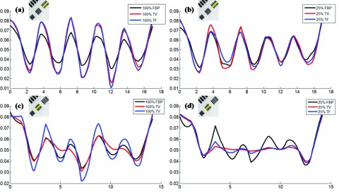
Cross-line plots for quantitative resolution analysis. (a) and (b) are for Bar 6 and 7 with 100% data; (c) and (d) are for Bar 6 and 7 with 25% data. The unit of x axis is mm, and the unit of y axis is cm⁻¹.

Table 1.

The FWHM results for Bar 6 and 7 in the resolution slice. (Unit: mm.)

Bar 6		FWHM	Bar 7		FWHM
100% data	FBP	1.81	100% data	FBP	1.93
	TV	1.75		TV	2.37
	TF	1.69		TF	1.79
25% data	FBP	2.06	25% data	FBP	2.20
	TV	2.00		TV	2.86
	TF	1.79		TF	2.59

For the quantitative contrast analysis, the contrast-to-noise ratio (CNR) values [i.e., |μ_t − μ_b|/(σ_t² + σ_b²)^0.5 with the averaged value μ_t/μ_b of the target/background, and the standard deviation σ_t/σ_b of the target/background], were listed in Table 2 for various ROIs (Fig. 8) of the contrast slice from the Siemens imaging quality phantom.

Table 2.

The CNR results for the contrast slice with ROIs shown in Fig. 5.

		ROI1	ROI2	ROI3	ROI4
100% data	FBP	4.28	3.23	1.22	0.86
	TV	4.55	4.26	2.32	2.29
	TF	4.57	4.16	2.28	2.31
25% data	FBP	3.56	2.12	0.64	0.47
	TV	4.24	3.77	1.59	1.51
	TF	4.39	4.02	2.01	2.09

Figure 8.

ROIs for quantitative contrast analysis.

RESULTS

Phantom studies

The reconstruction results from FBP, TV, and TF on a resolution slice and a contrast slice of the Siemens imaging quality phantom are shown in Figs. 23, respectively. The quantitative resolution results are given in Fig. 7 and Table 1, and the quantitative contrast results are given in Table 2 with ROIs in Fig. 8.

The quantitative calculation of signal-to-noise ratio (SNR) has not been presented here, since it is apparent from the images that TV and TF were better than FBP for both 100% data and 25% data. With 25% data, the TV image showed the prominent TV-specific cartoon-like artifacts, and thus the TF image had better SNR than the TV image.

In terms of the image resolution, suggested by Fig. 2, with 100% data, the TF image had the best image resolution in terms of FWHM, which was mainly due to the reduced background noise and the maintained fine feature through TF; for the larger Bar 6, the FBP had the worst image resolution due to the relatively large background noise; for the smaller Bar 7, the TV had the worst image resolution due to the diminished fine feature through TV. With 25% data, for the larger Bar 6, TF still provided the best image resolution; for the smaller Bar 7, FBP provided the best image resolution, and the image resolution was slightly degraded in TV and TF. These findings based on Fig. 2 were further confirmed through the cross-sectional plot in Fig. 7 and the quantitative FWHM values in Table 1. Note that, for Bar 6 with 25% data [Fig. 7c], although the min−max difference (of the second peak from left) from TV was larger than that of TF, its FWHM was also larger since its peak was flat.

In terms of the image contrast in CNR, suggested by Fig. 3 and the quantitative CNR values in Table 2, with both 100% and 25% data, TV and TF were better than FBP. Comparing TV and TF, with 100% data, TV and TF had comparable image CNRs; with 25% data, TF had better contrasts than TV, which was mainly due to the cartoon-like artifacts from TV.

To summarize, both the visual images and quantitative analysis suggested that TF was superior in terms of the SNR, the resolution, and the contrast. It was clear that TF outperformed TV in all above three aspects. However, it was observed from our reconstruction tests and the given example here that FBP sometimes had better image resolution than TF (TV as well) when the data were undersampled, which may be due to the smoothing effect of the image regularization. This will be addressed in our future work.

Patient studies

The image reconstruction results for a H&N patient slice and a prostate patient slice are shown in Figs. 45, respectively.

For both patient studies with 100% data, TF [Figs. 4c, 5c] provided better visual image quality than TV [Figs. 4b, 5b], which was in turn better than FBP [Figs. 4a, 5a]. In terms of SNR, TV and TF were comparable, and better than FBP. Due to the much improved SNR, the TV and TF images showed better anatomical visualization. However, as indicated by the red arrows in Fig. 4, for example, the cartoon-like piecewise-constant artifact was visible in the TV image, but not in the TF image. In this sense, the TF image was better than the TV image.

For both patient studies with 25% data, TF [Figs. 4f, 5f] also provided better visual image quality than TV [Figs. 4e, 5e], which was in turn better than FBP [Figs. 4d, 5d]. Again, the TV and TF images showed better anatomical visualization than FBP, due to the significantly reduced noise level. However, similar to the case with 100% data, as indicated by the red arrows in Fig. 4, for example, the cartoon-like piecewise-constant artifact was quite severe in the TV image. In comparison, such a TV-specific artifact was not observed for TF due to the use of the second-order derivative and the multilevel image regularization. On the other hand, the small object, as indicated by the red arrows in Fig. 5, for example, was still clearly visible for TF, and yet hard to identify in FBP due to the noise, or TV due to the cartoon artifact.

CONCLUSIONS AND DISCUSSIONS

We have proposed a novel TF-based image reconstruction technique that provides better image quality than FBP and TV for the MVCT imaging on TomoTherapy with full or undersampled projection views. In particular, the phantom and patient studies suggest that the tensor framelet method is robust for the low-dose imaging on TomoTherapy with 75% reduction of the projection views. In addition, our GPU-based solver enables rapid image reconstruction. For example, it took ∼2 min to reconstruct a 40-slice 1 mm-resolution 350 × 350 3D image with 200 projection views per slice and 528 detections per view.

The low-dose scan through the undersampled projection views here is equivalent to the scan with faster gantry rotation speed, assuming the constant pulse rate. Therefore, the SNR level is maintained for each view, although the overall SNR of the image may be reduced due to fewer views. Moreover, the faster-rotation scan with the improved imaging quality by the proposed TF algorithm from FBP or TV would reduce the motion artifact due to shorter scanning time.

The proposed method in this study leads to better MVCT image quality on TomoTherapy, while the imaging dose is maintained or reduced. In contrast, in Ref. 32, the image quality can also be improved by increasing pulse rate, yet with higher imaging doses delivered to the patients. Such high-dose MVCT image method may be limited to a fewer fraction courses, such as stereotactic body radiation therapy (SBRT). Our proposed TF-based reconstruction method, however, is expected to improve the imaging quality for both conventional and hypofraction treatment.

References

- Zelefsky M. J., Fuks Z., Happersett L., Lee H. J., Ling C. C., Burman C. M., Hunt M., Wolfe T., Venkatraman E. S., Jackson A., Skwarchuk M., and Leibel S. A., “Clinical experience with intensity modulated accelerated radiation therapy (IMRT) in prostate cancer,” Radiother. Oncol. 55, 241–249 (2000). 10.1016/S0167-8140(99)00100-0 [DOI] [PubMed] [Google Scholar]
- Butler E. B., Teh B. S., W. H.GrantIII, Uhl B. M., Kuppersmith R. B., Chiu J. K., Donovan D. T., and Woo S. Y., “SMART (simultaneous modulated accelerated radiation therapy) boost: A new accelerated fractionation schedule for the treatment of head and neck cancer with intensity modulated radiotherapy,” Int. J. Radiat. Oncol., Biol., Phys. 45, 21–32 (1999). 10.1016/S0360-3016(99)00101-7 [DOI] [PubMed] [Google Scholar]
- Mackie T. R., Holmes T., Swerdloff S., Reckwerdt P., Deasy J. O., Yang J., Paliwal B., and Kinsella T., “Tomotherapy: A new concept for the delivery of dynamic conformal radiotherapy,” Med. Phys. 20, 1709–1719 (1993). 10.1118/1.596958 [DOI] [PubMed] [Google Scholar]
- Meeks S. L., J. F.HarmonJr., Langen K. M., Willoughby T. R., Wagner T. H., and Kupelian P. A., “Performance characterization of megavoltage computed tomography imaging on a helical tomotherapy unit,” Med. Phys. 32, 2673–2681 (2005). 10.1118/1.1990289 [DOI] [PubMed] [Google Scholar]
- Ruchala K. J., Olivera G. H., Schloesser E. A., and Mackie T. R., “Mega-voltage CT on a tomotherapy system,” Phys. Med. Biol. 44, 2597–2621 (1999). 10.1088/0031-9155/44/10/316 [DOI] [PubMed] [Google Scholar]
- Murphy M. J., Balter J., Balter S., J. A.BenComoJr., Das I. J., Jiang S. B., Ma C. M., Olivera G. H., Rodebaugh R. F., and Ruchala K. J., “The management of imaging dose during image-guided radiotherapy: Report of the AAPM task group 75,” Med. Phys. 34, 4041–4062 (2007). 10.1118/1.2775667 [DOI] [PubMed] [Google Scholar]
- Brenner D. J. and Hall E. J., “Computed tomography: An increasing source of radiation exposure,” N. Engl. J. Med. 357, 2277–2284 (2007). 10.1056/NEJMra072149 [DOI] [PubMed] [Google Scholar]
- Hricak H., Brenner D. J., Adelstein S. J., Frush D. P., Hall E. J., Howell R. W., McCollough C. H., Mettler F. A., Pearce M. S., and Suleiman O. H., “Managing radiation use in medical imaging: A multifaceted challenge,” Radiology 258, 889–905 (2011). 10.1148/radiol.10101157 [DOI] [PubMed] [Google Scholar]
- Chan M. F., Yang J., Song Y., Burman C., Chan P., and Li S., “Evaluation of imaging performance of major image guidance systems,” Biomed. Imaging Interv. J. 7, e1–e7 (2011). [DOI] [PMC free article] [PubMed] [Google Scholar]
- Candès E. J., Romberg J., and Tao T., “Robust uncertainty principles: Exact signal reconstruction from highly incomplete frequency information,” IEEE Trans. Inf. Theory 52, 489–509 (2006). 10.1109/TIT.2005.862083 [DOI] [Google Scholar]
- Donoho D. L., “Compressed sensing,” IEEE Trans. Inf. Theory 52, 1289–306 (2006). 10.1109/TIT.2006.871582 [DOI] [Google Scholar]
- Sidky E. Y., Kao C.-M., and Pan X., “Accurate image reconstruction from few-views and limited-angle data in divergent-beam CT,” J. X-Ray Sci. Technol. 14, 119–139 (2006). [Google Scholar]
- Chen G. H., Tang J., and Leng S., “Prior image constrained compressed sensing (PICCS): A method to accurately reconstruct dynamic CT images from highly undersampled projection data sets,” Med. Phys. 35, 660–663 (2008). 10.1118/1.2836423 [DOI] [PMC free article] [PubMed] [Google Scholar]
- Yu H. Y. and Wang G., “Compressed sensing based interior tomography,” Phys. Med. Biol. 54, 2791–2805 (2009). 10.1088/0031-9155/54/9/014 [DOI] [PMC free article] [PubMed] [Google Scholar]
- Choi K., Wang J., Zhu L., Suh T.-S., Boyd S., and Xing L., “Compressed sensing based cone-beam computed tomography reconstruction with a first-order method,” Med. Phys. 37, 5113–5125 (2010). 10.1118/1.3481510 [DOI] [PMC free article] [PubMed] [Google Scholar]
- Jia X., Dong B., Lou Y., and Jiang S. B., “GPU-based iterative cone-beam CT reconstruction using tight frame regularization,” Phys. Med. Biol. 56, 3787–3806 (2011). 10.1088/0031-9155/56/13/004 [DOI] [PubMed] [Google Scholar]
- Gao H., Cai J. F., Shen Z., and Zhao H., “Robust principal component analysis-based four-dimensional computed tomography,” Phys. Med. Biol. 56, 3181–3198 (2011). 10.1088/0031-9155/56/11/002 [DOI] [PMC free article] [PubMed] [Google Scholar]
- Zhao B., Gao H., Ding H., and Molloi S., “Tight-frame based iterative image reconstruction for spectral breast CT,” Med. Phys. 40, 031905 (10pp.) (2013). 10.1118/1.4790468 [DOI] [PMC free article] [PubMed] [Google Scholar]
- Gao H., Li R., Lin Y., and Xing L., “4D cone beam CT via spatiotemporal tensor framelet,” Med. Phys. 39, 6943–6946 (2012). 10.1118/1.4762288 [DOI] [PMC free article] [PubMed] [Google Scholar]
- Gao H., “Fast parallel algorithms for the x-ray transform and its adjoint,” Med. Phys. 39, 7110–7120 (2012). 10.1118/1.4761867 [DOI] [PMC free article] [PubMed] [Google Scholar]
- https://sites.google.com/site/fastxraytransform.
- Rudin L., Osher S., and Fatemi E., “Nonlinear total variation based noise removal algorithms,” J. Phys. D 60, 259–268 (1992). 10.1016/0167-2789(92)90242-F [DOI] [Google Scholar]
- Tibshirani R., Saunders M., Rosset S., and Zhu J. “Sparsity and smoothness via the fused Lasso,” J. R. Stat. Soc. Ser. B (Stat. Methodol.) 67, 91–108 (2005). 10.1111/j.1467-9868.2005.00490.x [DOI] [Google Scholar]
- https://sites.google.com/site/spatiotemporaltensorframelet.
- Dong B. and Shen Z., “MRA based wavelet frames and applications,” Summer Program on The Mathematics of Image Processing, IAS Lecture Notes Series Vol. 19 (Park City Mathematics Institute, 2010).
- Goldstein T. and Osher S., “The split Bregman algorithm for l1 regularized problems,” SIAM J. Imaging Sci. 2, 323–343 (2009). 10.1137/080725891 [DOI] [Google Scholar]
- Gao H., Yu H., Osher S., and Wang G., “Multi-energy CT based on a prior rank, intensity and sparsity model (PRISM),” Inverse Probl. 27, 115012 (2011). 10.1088/0266-5611/27/11/115012 [DOI] [PMC free article] [PubMed] [Google Scholar]
- Cai J. F., Osher S., and Shen Z., “Split Bregman methods and frame based image restoration,” Multiscale Model. Simul. 8, 337–369 (2009). 10.1137/090753504 [DOI] [Google Scholar]
- Gayou O. and Miften M., “Commissioning and clinical implementation of a mega-voltage cone beam CT system for treatment localization,” Med. Phys. 34, 3183–3192 (2007). 10.1118/1.2752374 [DOI] [PubMed] [Google Scholar]
- Moore K. L., Palaniswaamy G., White B., Goddu S. M., and Low D. A., “Fast, low-dose patient localization on TomoTherapy via topogram registration,” Med. Phys. 37, 4068–4077 (2010). 10.1118/1.3453577 [DOI] [PubMed] [Google Scholar]
- Buzug T. M., Computed Tomography: From Photon Statistics to Modern Cone-Beam CT (Springer, Verlag Berlin Heidelberg, 2008). [Google Scholar]
- Westerly D. C., Schefter T. E., Kavanagh B. D., Chao E., Lucas D., Flynn R. T., and Moyed M., “High-dose MVCT image guidance for stereotactic body radiation therapy,” Med. Phys. 39, 4812–4819 (2012). 10.1118/1.4736416 [DOI] [PubMed] [Google Scholar]