Bayesian Tests of Topology Hypotheses with an Example from Diving Beetles

Abstract

We review Bayesian approaches to model testing in general and to the assessment of topological hypotheses in particular. We show that the standard way of setting up Bayes factor tests of the monophyly of a group, or the placement of a sample sequence in a known reference tree, can be misleading. The reason for this is related to the well-known dependency of Bayes factors on model-specific priors. Specifically, when testing tree hypotheses it is important that each hypothesis is associated with an appropriate tree space in the prior. This can be achieved by using appropriately constrained searches or by filtering trees in the posterior sample, but in a more elaborate way than typically implemented. If it is difficult to find the appropriate tree sets to be contrasted, then the posterior model odds may be more informative than the Bayes factor. We illustrate the recommended techniques using an empirical test case addressing the issue of whether two genera of diving beetles (Coleoptera: Dytiscidae), Suphrodytes and Hydroporus, should be synonymized. Our refined Bayes factor tests, in contrast to standard analyses, show that there is strong support for Suphrodytes nesting inside Hydroporus, and the genera are therefore synonymized. [Bayes factor; Coleoptera; Dytiscidae; marginal likelihood; model testing; posterior odds; reversible-jump MCMC; stepping-stone sampling.]

Testing hypotheses about the structure of trees is one of the most fundamental tasks in phylogenetic systematics. It helps answer questions such as: Does an unknown sample X belong to a known reference group A? Can two taxa A and B be maintained as separate or is one nested inside the other? Is clade A more closely related to clade B than to clade C? Is taxon A monophyletic?

Bayesian statistics includes several tools for comparing and testing models, and they have been applied to the testing of tree hypotheses in a number of recent papers (e.g., Lavoué et al. 2007; Marek and Bond 2007; Parker et al. 2007; Azuma et al. 2008; Rabeling et al. 2008; Yamanoue et al. 2008; Pavlicev et al. 2009; Tank and Olmstead 2009; Zakharov et al. 2009; Makowsky et al. 2010; Yang et al. 2010; Kelly et al. 2011; Knight et al. 2011; Schweizer et al. 2011; Drummond et al. 2012; Miller and Bergsten 2012). However, it is quite difficult to formulate relevant hypotheses about tree structure, and Bayes factor tests, as commonly applied in the literature, can be quite misleading. The purpose of this article is to discuss the Bayesian techniques for testing tree hypotheses, point out potential pitfalls, and provide general recommendations for empiricists. We illustrate both the pitfalls and the recommended techniques in a test of whether two genera of diving beetles (Coleoptera: Dytiscidae), Suphrodytes Gozis and Hydroporus Clairville, can be maintained as separate genera or should be synonymized.

Theory

Bayesian Model Testing

We will assume that the reader is familiar with the basics of Bayesian phylogenetic inference (see, e.g., Holder and Lewis 2003; Yang 2006; Ronquist and Deans 2010). For an introduction to statistical testing of phylogenetic models in general, see Sullivan and Joyce (2005). The theory of Bayesian model testing was worked out primarily by Jeffreys (1935, 1961). An excellent summary of the early work on Bayesian model testing is provided by Kass and Raftery (1995), who also laid the foundation for much of the modern work in the field.

In Bayesian inference we are interested in the posterior probability of model parameters (θ) given some observed data (D) and a model (M). The posterior probability f (θ|D,M) is obtained from the prior probability f (θ|M) of the parameter values, and the probability of the data given the parameter values and the model f (D|θ,M) (also called the “likelihood”), by Bayes' theorem

The normalizing constant in Bayes' theorem, f (D|M), is the marginal likelihood of the data. It is also the predictive probability of the data: the probability of seeing the observed data calculated from the model before the data are taken into account (Kass and Raftery 1995). Sometimes it is called the marginal [model] likelihood or the integrated [model] likelihood; we will refer to it simply as the model likelihood.

It is this model likelihood, which is used in Bayesian model comparison. Assume we have two models, M₁ and M₂. If we specified the prior probabilities of the two models, f (M₁) and f (M₂), we could calculate the posterior odds of the models as

The last ratio is the ratio of the model likelihoods, also known as the Bayes factor. We could thus specify the same equation in words as

Both posterior model odds and Bayes factors are used to compare models in Bayesian inference. When two or more models are considered in the same analysis, it is natural to focus on the marginal probabilities of the models, f (M₁ |D ), in the posterior of the supermodel analysis. This is how you would approach inference about any other discrete parameter in the analysis. The posterior model odds are simply the ratio between the marginal model probabilities.

A possible disadvantage of posterior model odds is that they depend on the prior on models. We can get rid of this dependency by focusing on the Bayes factor. Even the Bayes factor, however, is sensitive to the priors on model-specific parameters (as opposed to the prior probabilities of the models themselves). For instance, if one model is a special case of the other, then the Bayes factor is dependent on how focused the prior is on the larger parameter space (Kass and Raftery 1995 and references cited therein). It is an analogous effect that can cause problems with Bayes factor tests of topological hypotheses, as we will discover.

One way of understanding the Bayes factor is that it measures the strength of the data in changing the prior model odds. Alternatively, because the model likelihood is the predictive probability of the data, we can also view the Bayes factor as measuring the relative success of the models in predicting the data (Kass and Raftery 1995). The Bayes factor is closely related to the likelihood ratio statistic: change the integrated likelihoods to maximized likelihood and you essentially have the latter. Unlike the likelihood ratio statistic, however, Bayes factors can be used on any pair of models, regardless of whether or not they are nested. The former statistic is based on a chi-square distribution, taking the number of parameters into account through the degrees of freedom. Bayes factors, in contrast, have a natural way of penalizing overfitting, “a fully automatic Occam's razor” (Kass and Raftery 1995).

Based on the similarity to the likelihood ratio statistic, general guidelines to the interpretation of Bayes factors were suggested by Kass and Raftery (1995). Specifically, they indicated that a Bayes factor larger than 3 should be interpreted as significant positive evidence in favor of the better model. A scale similar to the likelihood ratio statistic is obtained by taking twice the logarithm of the Bayes factor; on this scale, the critical value is 2 (Table 1).

Table 1.

Interpretation of the Bayes factor for hypothesis testing after Kass and Raftery (1995)

Bayes factor	2×loge BF	Interpretation
1–3	0–2	Not worth more than a bare mention
3–20	2–6	Positive
20–150	6–10	Strong
> 150	>10	Very strong

Computational Challenges

There are two main approaches to estimating posterior model odds and Bayes factors. The first one is to use a single Markov chain Monte Carlo (MCMC) analysis to estimate the posterior model probabilities (for phylogenetic examples, see Suchard et al. 2001, 2005; Huelsenbeck et al. 2004). If the models have a different number of dimensions, or include different parameters, then one has to implement reversible-jump MCMC, which is technically demanding. It can also be difficult to obtain good mixing across complex model spaces. Despite the difficulties, this is often the best approach for estimating moderate to large model probabilities. Small model probabilities, however, are difficult to estimate precisely. This means that more extreme posterior model odds are difficult to assess reliably. If the aim is to estimate Bayes factors, and the analysis uses prior model odds that are strongly biased, the results can be severely compromised as will be shown below. A possible solution is to modify the prior probabilities of models until the models of interest receive similar posterior probabilities. Bayes factors or posterior model odds can then be computed by taking the modified prior probabilities into account. Suchard et al. (2005) developed this approach further, referring to it as “Bayes factor titration”.

The other approach involves separate estimation of each of the model likelihoods. This means running a complete MCMC simulation on each model, so it can only be successfully applied to a small number of models. In addition, it is extremely difficult to estimate the model likelihood, which is typically a sum and integral over a large and complex parameter space. The most commonly used estimator is the harmonic mean estimator (HME) (Newton and Raftery 1994), which is simply the harmonic mean of the likelihoods of the MCMC output. The HME is sensitive to the inclusion of rare values with large influence on the estimate, and it tends to overestimate the model likelihood. More accurate estimates of the model likelihood can be obtained by thermodynamic integration (Lartillot and Philippe 2006), also known as path sampling (Baele et al. 2012), or the so-called stepping-stone method (Fan et al. 2011; Xie et al. 2011) albeit at a significantly increased computational cost.

Bayesian Tests of Tree Hypotheses

In Bayesian phylogenetic inference, the tree is often viewed as a discrete parameter, which can take on many different values, one for each tree topology. However, mapping parameters associated with nodes or branches, such as branch lengths, from one tree to another is not straightforward. In some sense, all nodes and branches of two distinct tree topologies are different regardless of how similar the topologies are or how many bipartitions they share.

Inspired by this, some workers consider each topology as a separate model (e.g., Suchard et al. 2001, 2005; Yang 2006) instead of treating the topology as an ordinary discrete model parameter. This leads to the view that a typical Bayesian phylogenetic analysis is a case of reversible-jump MCMC across topology model space. This is the view we will adopt here. If we only consider fully resolved trees, then the dimension of each model is the same but the node and branch length parameters are not identical. Thus, each jump between models amounts to discarding some parameters (dimensions) and adding in an equal number of other parameters (dimensions).

From an ordinary Bayesian phylogenetic analysis, then, we get the marginal posterior probabilities of the topology models. To get the posterior model odds for two distinct topologies, we simply divide the frequency of one tree with the frequency of the other in our sample of the posterior.

In inference of non-clock trees, it is standard procedure to associate each distinct topology with the same prior probability, in which case the posterior odds are the same as the Bayes factor. For clock trees, the standard models (birth–death, coalescent, uniform) typically put equal prior probability on unique labeled histories rather than on unique topologies. To calculate the Bayes factor for two distinct rooted topologies then, one has to take into account that they may be compatible with different numbers of labeled histories (Felsenstein 2004). For a simple example, consider a four-taxon clock tree. There are two histories compatible with a symmetric topology, depending on which speciation event happened first. In contrast, there is only one possible sequence of speciation events in an asymmetric, comb-like topology. If the prior puts equal probability on all speciation histories, then symmetric topologies are twice as likely as asymmetric ones. To obtain Bayes factors from a posterior sample of trees under these conditions, simply divide the frequency of symmetric topologies with two to correct for the topology bias in the prior, and then use the ratio between the corrected frequencies. Except for this correction, topological hypothesis tests on clock trees behave essentially the same as tests on non-clock trees.

An important problem is that topology space is huge for even moderate numbers of taxa, and the posterior probabilities of an individual topology is likely to be small and difficult to estimate accurately. Even the best topologies may individually have low posterior probability in a large analysis. It is arguably easier to estimate the posterior probabilities of classes of trees than it is to assess the probability of individual topologies.

Focusing on classes of trees leads to other problems, however (for a discussion of similar problems from a different perspective, see Wheeler and Pickett 2008). When using Bayes factors, for instance, the hypotheses of interest are often associated with very different numbers of topologies (see below). In fact, the vastness of tree space often produces such extreme prior odds in standard analyses that it becomes hopeless in many cases to estimate Bayes factors from the posterior model odds. For instance, the prior odds might be so biased in favor of a particular clade being monophyletic that it would take an enormously large MCMC sample to show that the posterior odds are higher than the prior odds. One possibility is then to restructure the prior by introducing partition-associated probability factors and then do Bayes factor titration (Suchard et al. 2005; see also Ronquist et al. 2004).

A more serious problem, however, is to identify the relevant classes of trees to be contrasted. This is surprisingly difficult and can lead to counter-intuitive results, especially when using Bayes factors. In fact, we argue here that the Bayes factor test of topological hypotheses used today by most phylogeneticists (in the following referred to as “standard Bayes factor tests”) should be abandoned in favor of more appropriate techniques. The problem is related to the sensitivity of Bayes factors to model-specific priors, and will be illustrated here with two hypothetical examples.

Consider first the problem of determining whether or not a sample sequence X belongs to a known group A, a problem analysed by Suchard et al. (2005). Assume for simplicity that the monophyly of A (without considering X) is overwhelmingly supported by the data. Further assume that there is no evidence allowing us to place X; all placements of X in the tree results in the same likelihood. Under these circumstances, the Bayes factor should be 1, that is, there should be no evidence for or against the hypothesis that X belongs to A compared to the hypothesis that X does not belong to A.

The standard approach explored by Suchard et al. (2005) would be to test the hypothesis that X+A form a monophyletic group (H₁) against the hypothesis that they do not (H₀). This will likely produce misleading results, as we will see in the following. In the tree without X, let a be the number of taxa in A, and n the number of taxa in total. If A is a non-trivial group in the tree without X, then we have a ≤ n−2 (group A excludes at least two taxa). Further, let B(n) be the number of unrooted, fully resolved trees for n taxa. If the prior associates each tree with the same prior probability, the prior odds for H₁ against H₀ would be

For large n, the denominator is close to 1, so this ratio is very nearly equal to

In the posterior, we expect all or almost all trees to have A as monophyletic. Given that this is true, and that X can be placed with equal probability on every branch in the tree, the posterior odds of X being placed inside A whereas it being placed outside is simply the ratio between the number of branches in A and the number of branches outside A,

Since the Bayes factor is the posterior odds divided by the prior odds, we obtain the Bayes factor as

This is guaranteed to be a large number, especially for large n, suggesting that there is significant support for H₀. In other words, the Bayes factor is misleading. The reason for this counter-intuitive result is that the Bayes factor reflects both the strength of evidence in favor of placing X in A, and the evidence in favor of monophyly of A regardless of the position of X. Given the way the problem is formulated, we should take strong evidence for the monophyly of A for granted, and account for that in the hypothesis test.

Because such background information is often reflected in the posterior, the posterior odds can be more informative than Bayes factors calculated in the standard way. For instance, in this particular case, the posterior odds for X grouping with A would be

This will not deviate much from 1, so the posterior odds will suggest that there is little evidence for placing X inside A. However, the odds will be exactly equal to 1 only when there are as many tree tips inside as outside of A (a = n–a, and assuming that placement as sister to A is indecisive).

To calculate a meaningful Bayes factor for this problem, we need to restrict our attention to trees that have A monophyletic after pruning of X. In the best case, all the trees in the posterior sample from an unconstrained analysis will satisfy this constraint, in which case the posterior tree sample can be used directly for the calculation of Bayes factors. If only some trees in the posterior sample violate the constraint, we can filter them out, for instance using a backbone constraint in PAUP, and then use the remaining trees for hypothesis testing. One can also run an MCMC analysis using a backbone constraint forcing A to be monophyletic regardless of the position of X, as permitted, for example, in the most recent version of MrBayes (Ronquist et al. 2012), and then use this tree sample for model testing.

An alternative, but likely less accurate method, is to estimate the model likelihood separately for the two hypotheses. One would then run an analysis with A constrained to be monophyletic without X. The other analysis would have A+X constrained to be monophyletic, and A without X constrained not to be monophyletic. The latter constraint is important if X being the sister of A is not considered part of the tree set relevant for H₁.

If we restrict our attention to the backbone trees with A monophyletic, then the prior odds for X being placed inside A would be

This is the same as the posterior odds, and thus gives the expected Bayes factor of 1. Essentially, what we have done is to take the background information that A (with or without X) is likely to be monophyletic into account in the topology prior, making the Bayes factor test informative rather than misleading. This illustrates how sensitive Bayes factor tests of topology hypotheses are to the specification of the topology prior, unlike posterior model odds. Unfortunately, the standard flat prior on topologies (or histories) is rarely appropriate for Bayes factor tests of topological hypotheses.

For a second example of the problems with standard Bayes factor tests of topological hypotheses, consider the very common question of whether a group A is monophyletic. Also here it is easy to get contradictory results if one does not consider the relevant tree classes carefully. This can be illustrated with a simple example (Fig. 1). Assume that A consists of two subgroups, A₁ and A₂, which are both overwhelmingly supported as monophyletic, while there is no evidence concerning the relationships in the rest of the tree. The hypothesis test should then tell us that there is no evidence for or against the hypothesis that A is monophyletic.

Figure 1.

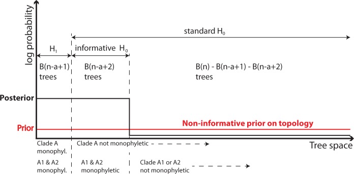
Schematic illustration of the Bayes factor test of the hypothesis that A is a monophyletic group (H₁) against the hypothesis that it is not (H₀). We assume that A consists of two strongly supported subclades, A1 and A2, but that the rest of the tree is unresolved such that there is no evidence that A1 and A2 together form a monophyletic group. The Bayes factor compares the average height of the posterior over the prior tree space of each hypothesis. When using a standard H₀, the signal is spread over a large tree space, and the test suggests that H₁ is strongly supported. If we use an informed prior for H₀ by restricting the tree space to those trees that have A1 and A2 monophyletic, then the Bayes factor correctly identifies that there is no support for or against H₁ over H₀, as the average height is the same. A posterior odds test compares the total probability mass under each hypothesis (the area under the posterior distribution), and is therefore not as strongly influenced by the size of the tree space as the Bayes factor.

We first consider the standard hypothesis test where we contrast A being monophyletic (H₁) with A not being monophyletic (H₀). As before, we have a taxa in A₁ + A₂, n taxa in the tree in total and a ≤ n−2. The prior odds for A being monophyletic are very nearly

which is a very small number if n is large. If we consider the tree outside of A₁ and A₂, there will be n − a + 2 tips in it (two tips representing A₁ and A₂, respectively). There will be B(n−a+2) equally well-supported trees, only B(n−a+1) of which will have A monophyletic. The posterior odds for A being monophyletic will then be

since we know in general that B(n+1) = (2n−3)B(n).

This gives a Bayes factor of

which is guaranteed to be a large number for large n. Again, the standard Bayes factor test is misleading, and just using the posterior odds as a guide is more informative. Even better is to take the monophyly of A₁ and A₂ into account in both H₁ and H₀, in which case we get the expected Bayes factor of 1 (Fig. 1).

What if there is also structure in the outgroup? Let the outgroup consist of two groups B₁ and B₂ with a total of b species. Furthermore, assume that there is no information about the structure of the tree except that A₁, A₂, B₁, and B₂ are each strongly supported as monophyletic. The prior odds for A being monophyletic are the same but the posterior odds are going to be much higher (less extreme) because there are more constraints on outgroup relationships. It could be as high as 1/3, if n = a+b. Specifically, the Bayes factor is going to be

Thus, the effect is to make the Bayes factor larger, resulting in the standard test being even more misleading.

We now turn our attention to a specific empirical case that illustrates the difficulties described above. In the discussion, we return to how these observations can be used to provide general recommendations for Bayesian tests of tree hypotheses.

Empirical Example

The Northern Hemisphere genus Hydroporus is with its over 180 known valid species dominating the tribe Hydroporini. Most species of the genus inhabit boreal and arctic wetlands where they form an important part of the fauna as predators of zooplankton and benthic insect larvae, especially in the shallower parts of more temporary waters. The delimitation of the genus relative to a number of other smaller genera of the tribe remains problematic, as well as the recognition of subgenera within the genus, at present abandoned in favor of a less formal classification into 29 species groups (Nilsson 2001). Recent trends in the delimitation of Hydroporus include both splitting, like the recognition of Hydrocolus Roughley and Larson as a separate genus, as well as lumping such as the synonymization of Hydrotarsus Falkenström with Hydroporus (Ribera et al. 2003).

Here we primarily want to test the monophyly of Hydroporus relative to the Palearctic genus Suphrodytes, with its traditionally recognized single species recently split into two (Bergsten et al. 2012). Suphrodytes was introduced by Gozis (1914) as a subgenus of Hydroporus, including the single species Hydroporus dorsalis (Fabricius). Later authors largely accepted the new subgenus but gradually added a number of other northern large-bodied Hydroporus species to the group (Zimmermann 1931; Guignot 1932, 1947; Balfour-Browne 1938; Zaitzev 1953). This association was later abandoned by Angus (1985), who stressed the isolated position of dorsalis, adding to characters from the prosternal process also characters from the female genital tract, and changed the status of Suphrodytes to a monobasic genus. This view was to be accepted by most subsequent authors publishing on European Hydroporini (Nieukerken 1992; Nilsson and Holmen 1995; Nilsson 2001, 2003).

More recently, the molecular phylogenetic analysis of Ribera et al. (2003, 2008) and Hernando et al. (2012) suggested that Suphrodytes dorsalis was nested within Hydroporus, providing evidence in favor of a synonymization of Suphrodytes with Hydroporus. However, Ribera et al. (2003) and Hernando et al. (2012) only used mitochondrial markers and support for the conclusion was weak or algorithm dependent and hence no formal change to the classification was made by either. (Ribera et al.'s , 2008) analysis used both nuclear and mitochondrial genes but focused on the higher-level relationships within the family Dytiscidae and the sample was too sparse at the species group level to make any definite conclusions regarding Suphrodytes and Hydroporus. Only four of the 29 species groups of Hydroporus were represented in that study. As taxonomic sampling is imperative for accurate phylogenetic estimation (Zwickl and Hillis 2002; Heath et al. 2008) solving the Suphrodytes/Hydroporus controversy will require a study focused on the Hydroporus group of genera, a much broader sample of Hydroporus species groups, both nuclear and mitochondrial genes and explicit topological hypothesis testing.

Approach Taken Here

In this study we expand the four-gene dataset of Ribera et al. (2008) to include representatives of > 75% of species groups in Hydroporus for the focused question of the phylogenetic placement of Suphrodytes in relation to Hydroporus. In a Bayesian hypothesis-testing framework we use a recently improved method of marginal likelihood estimation to explicitly test competing topologies using the Bayes factor. We show that the standard approach to calculating the Bayes factor results in the opposite conclusion compared to our preferred approach outlined above. We also calculate the posterior model odds for the alternative hypotheses by filtering the tree sample from the MCMC analysis, which supports the conclusion of our preferred Bayes factor approach. A common practice to estimate the marginal likelihood of models is to use the harmonic mean of the log likelihood from MCMC analyses (e.g., Nylander et al. 2004; Miller et al. 2009; see original Newton and Raftery 1994), conveniently part of the output of popular software like MrBayes 3.1 (Ronquist and Huelsenbeck 2003). However it is known that the harmonic mean is a poor estimator and substantially overestimates the marginal likelihood of the model (Lartillot and Philippe 2006; Xie et al. 2011). Instead we used the stepping-stone sampling method recently described by Xie et al. (2011), which has been shown to be significantly more accurate than the harmonic mean method.

Materials and Methods

Taxon Sampling

We restricted the taxon sampling to the Hydroporus group of genera as defined by Ribera et al. (2008) in their Figure 3 labeled as node number 26 of well-supported nodes. This included apart from Suphrodytes and Hydroporus also Neoporus Guignot, Heterosternuta Strand, Hydrocolus, and Sanfilippodytes Franciscolo. From Ribera et al.'s analysis we consider it unambiguous that Suphrodytes belong nowhere else outside this group of genera and a test of its placement can be restricted to this subgroup within Hydroporinae. As outgroups to root the tree we used Andex insignis Sharp, Hyphydrus ovatus (Linnaeus), Hovahydrus minutissimus (Régimbart), Canthyporus hottentottus (Gemminger and Harold) and Laccornellus copelatoides (Sharp) which were part of the two closest clades to the Hydroporus group in Ribera et al. (2008). Within Suphrodytes we sampled the two existing species, S. dorsalis and Suphrodytes figuratus (Gyllenhal) after a recent treatment showing the genus is not monotypic as previously believed (Bergsten et al. 2012). Within Hydroporus we sampled representatives of as many additional species groups as possible to the ones included in Ribera et al. (2008), in particular some of the large-bodied species historically associated with Suphrodytes . This resulted in adding 19 new groups to Ribera et al.'s four to a total of 23 of the 29 presently recognized species groups being represented in the final data matrix (Appendix).

FIGURE 3.

Phylogeny based on the combined four-gene matrix from the unconstrained Bayesian analysis and rooted between outgroups and ingroups as defined a priori. Numbers refer to posterior probability clade support values.

DNA Extraction, PCR, and Sequencing

For most species DNA was extracted from the head and prothorax in 96-well Wizard SV plates following the manufacturer's instructions (Promega). A few additional species were extracted from one hindleg with a GeneMole automated extraction robot (Mole Genetics AS). We targeted two nuclear (18 s and H3) and two mitochondrial (CO1 and 16s) genes for the analysis using the primers listed in Supplmentary Table S1 (doi:10.5061/dryad.s631d). For H3, 16 s, and 18 s we used Ready-ToGo™ PCR beads (Amersham Biosciences) in a 25 ul reaction volume with a 0.4 uM concentration of each primer and 2 ul of DNA (unknown concentration). Cycling conditions started with a 5 min denaturation step at 95°C followed by 40 cycles of 30 s at 95°C, 30 s at 50°C, and 60 s at 72°C, followed by a final extention step of 8 min at 72°C. Most CO1 sequences were amplified with Bioline Taq instead of beads but with the same primer and DNA concentration. Cycling condition for CO1 was 94° for 2 min, 35–40 cycles of 94° for 30 s, 51°–53° for 60 s and 70° for 90 s–120 s, and a final extension of 70° for 10 min. Most PCR products were purified with Exonuclease I and FastAP (Fermentas) in the proportion 1:4, and sequenced with a BigDye™ Terminator ver. 3.1 Cycle Sequencing Kit (Applied Biosystems), cleaned with a DyeEx 96 kit (Qiagen) and run on an ABI Prism 3100 Genetic Analyzer (Applied Biosystems). Some CO1 products were cleaned with a 96-well Millipore multiscreen plate and sequenced in both directions using a BigDye™ Terminator ver. 2.1, and analysed on an ABI 3730 automated sequencer.

Analyses and Hypothesis Testing

Sequence chromatograms were edited, trimmed of the primer ends and exported as fasta files in Sequencher v. 4.8 (Gene Codes Corporation). New DNA sequences are submitted to Genbank under the accession codes JX434757- JX434840 (Appendix). Sequences were aligned in Clustal X v. 2.0.12 (Larkin et al. 2007) with default gap opening and gap extension penalties (15 and 6.66, respectively). The alignments of the length-variable ribosomal genes were compared with using Mafft v. 6.850 (Katoh and Toh 2008) (E-INS-i, L-INS-I, and G-INS-i, all with 10 iterations) but differences were minimal (1 bp in length, 0.003 and 0.022 difference in posterior probability branch support for the placement of Suphrodytes in single-gene analyses of 16 s and 18 s, respectively) and the clustal alignments were used for all four genes. The parallel mpi version of MrBayes version 3.2 (build 457) (Altekar et al. 2004; Ronquist et al. 2012) was used to infer a phylogenetic hypothesis from the combined four-gene dataset. We specified a partitioned model based on genes and codon positions. For each partition we specified a model a priori allowing for the estimation of base frequencies, the proportion of invariable sites and allowed for rate-variation across sites with a gamma distribution. However, the core of the model, the substitution rate matrix, was not specified a priori. Instead we used reversible-jump MCMC to integrate over the pool of all 203 possible reversible 4×4 nucleotide models. The method was first described by Huelsenbeck et al. (2004) and has been implemented in the latest version of MrBayes 3.2 (Ronquist et al. 2012). All parameters were unlinked across partitions except topology and branch length, and each partition also had separate relative rate multipliers. Other prior and proposal settings were left as default. Ten million MCMC generations were sampled every 1000th step and the first 25% were discarded as burn-in. We ran four independent runs each with one cold and one heated chain (T = 0.2) and pooled the samples after burn-in was removed. Mixing and convergence was monitored through the statistics provided in the program. The tree was rooted between the ingroup and outgroups as specified a priori unless non-monophyly of the ingroup prevented such a rooting.

We specified two hypotheses to be tested against each other. Traditional classification treats Hydroporus and Suphrodytes as two separate and valid genera and this constitutes our null-hypothesis H₀: Hydroporus is monophyletic exclusive of Suphrodytes. The alternative hypothesis H₁ specifies a paraphyletic Hydroporus with Suphrodytes nested within Hydroporus, something that has been suspected because of weak morphological synapomorphies of Hydroporus and also indicated by some molecular data, albeit poorly sampled for Hydroporus (e.g., Ribera et al. 2008), or algorithm dependent and based on mitochondrial data (Hernando et al. 2012). We used the two approaches to Bayesian hypothesis testing as described above: Bayes factor and posterior model odds. The posterior probability for H₀ and H₁ was calculated by filtering the posterior tree sample in PAUP* v. 4.0a125 (Swofford 2002) and calculating the frequency of trees congruent with respective hypothesis. We do this both for the tree sample from an unconstrained analysis and for the tree sample from a backbone-constrained analysis where Hydroporus is constrained to be monophyletic with respect to other Hydroporini (both ingroup and outgroup taxa) but Suphrodytes is allowed to “float” without constraints. The latter approach focuses the hypothesis testing to only involve Suphrodytes in relation to Hydroporus without the interference of other Hydroporini-taxa in relation to Hydroporus. For the Bayes factor test we contrast what we call the standard approach with our preferred approach and show that it changes the outcome of the test. In the standard test we calculate the marginal likelihood of H₀ by using an absolute monophyly constraint on Hydroporus as an informed topology prior, whereas the marginal likelihood of H₁ was calculated from an unconstrained analysis with an uninformative prior across topology space. This is the approach taken in many empirical studies (e.g., Lavoué et al. 2007; Marek and Bond 2007; Parker et al. 2007; Azuma et al. 2008; Yamanoue et al. 2008; Pavlicev et al. 2009; Tank and Olmstead 2009; Makowsky et al. 2010; Yang et al. 2010; Knight et al. 2011). In our preferred Bayes factor test we calculate the marginal likelihood of the alternative hypotheses after specifying equally informed priors (constraints) on the topology (Fig. 2).

Figure 2.

Comparison of standard (a–b) and preferred (c–d) Bayesian hypothesis testing for the empirical example. Standard: When the H₀ hypothesis a) of a paraphyletic Hydroporus is tested as unconstrained against the alternative H₁ hypothesis b) constrained to comply with a monophyletic Hydroporus, the latter is strongly preferred by the Bayes factor (2×log_e BF = 88.96 in favor of H1). However, this is largely due to strong signal for the two subclades within Hydroporus. Preferred: When the H₀ hypothesis c) of a paraphyletic Hydroporus is associated with an informed topology prior comparable to that of H₁ d), the Bayes factor instead prefers H₀ (2 × log_e BF = 7.82 in favor of H0). This is also the hypothesis with the largest posterior probability.

To calculate the marginal likelihood of models we used the stepping-stone sampling method of Xie et al. (2011), which is now implemented in MrBayes 3.2 (Ronquist et al. 2012). We used a value (0.4) for the α-shape parameter of the beta distribution within the range Xie et al. (2011) found optimal and 204,000 MCMC steps were sampled every 100th generation for each of 48 ß-values between 1 (posterior) and 0 (prior) after an initial 204,000 generations were discarded as burn-in. The contribution to the marginal likelihood from each step is estimated from a sample-size of 2040. The same setting was used for four independent runs for each model to be tested, each with one cold and one heated chain, and the arithmetic mean across runs of the estimated marginal likelihood for each model was used to calculate the Bayes factor. For all analyses, the chains and runs were distributed across eight cores of two 2.8 GHz Quad-Core Intel Xeon processors.

Results

DNA extraction, PCR and sequencing was successful for all 21 taxa and four genes added to the dataset resulting in no complete gene gaps in the alignment. The combined datamatrix consisted of 2111 aligned nucleotides of which 553 varied and 1558 were constant (Supplementary Table S2). The separate runs of the Bayesian analyses converged unproblematically to an average deviation of split frequencies of < 0.005, and the post burn-in, merged, runs resulted in the fully resolved topology shown in Figure 3. The tree could be rooted between ingroup (posterior probability, pp = 0.99) and outgroups as specified a priori. In the ingroup, Hydrocolus came out as sister to the remaining genera, but this must be seen as a tentative hypothesis as the support was just on the margin (pp = 0.51) to be recovered in the majority-rule consensus of the sampled trees. At this low level of support the recovered resolution is often sensitive to model specification. Hydrocolus apart, Heterosternuta+ Neoporus+Sanfilippodytes formed a strongly supported monophyletic group (pp = 0.99) sister to Hydroporus+Suphrodytes. Hydroporus and Suphrodytes were also highly supported as monophyletic (pp = 0.98). Within that clade, Hydroporus came out as paraphyletic due to Suphrodytes being nested inside with a posterior probability of 0.87. Hydroporus was divided into two well-supported monophyletic groups, here labeled Clade I and II. Clade I (pp = 0.98) included the following species groups: angustatus, fuscipennis, longulus, memnonius, neglectus, nigrita, puberulus, striola, tesselatus and tristis. Clade II (pp = 1.0) included the appalachius, axillaris, columbianus, erythrocephalus, lapponum, nigellus, niger, notabilis, obscurus, rufifrons, sinuatipennis, subpubescens, and transpunctatus species groups. Suphrodytes came out as sister group to Clade II with rather strong support (pp = 0.87). In the backbone-constrained analysis where Hydroporus was constrained to be monophyletic in relation to all taxa except “floating” Suphrodytes, the support for Suphrodytes+Hydroporus increased marginally to 1.0 and Suphrodytes+Hydroporus Clade II to 0.88.

Filtering the merged, post-burn-in, sample of trees for trees consistent with each hypothesis resulted in a posterior model odds of H₁ versus H₀ of 0.947/0.0334 for the unconstrained analysis and 0.9662/0.0338 for the backbone-constrained analysis (Table 2). According to the posterior model odds there was hence about 28 times higher probability for the hypothesis H₁ of a paraphyletic Hydroporus without Suphrodytes to the hypothesis H₀ of a monophyletic Hydroporus.

Table 2.

Posterior probability of hypotheses based on an unconstrained analysis and a backbone-constrained analysis where Hydroporus is constrained monophyletic in relation to the outgroups but Suphrodytes is allowed to “float”

Constraints	H0	H1	H2	H3
Unconstrained	0.03339	0.86825	0.08666	0.9469
(30,004)	(1018)	(26,050)	(2601)	(28,411)
Backbone	0.03376	0.88025	0.08582	0.9662
(30,004)	(1013)	(26,410)	(2576)	(28,991)

Notes: H₀ = Hydroporus monophyletic to the exclusion of Suphrodytes; H₁ = Suphrodytes+Hydroporus Clade II monophyletic; H₂ =Suphrodytes +Hydroporus Clade I monophyletic; H₃ = Suphrodytes nested within Hydroporus. In parenthesis the total number of trees filtered out from the total (30,004) that supports the hypothesis.

The stepping-stone MCMC sampling converged successfully among the four independent runs for all 48 ß-values with an average deviation of split frequencies always < 0.03. The standard Bayes factor test estimated the marginal likelihood for H₁ from an unconstrained analysis and for H₀ under the topological constraint of Hydroporus monophyly. The estimation of the marginal log likelihood was −13,366.34 for the null hypothesis and −13,410.82 for the unconstrained H₁ hypothesis (Table 3). The test statistic 2×log_e BF = 88.96 which, according to the scale of interpretation (Table 1), gives very strong support in favor of the constrained hypothesis (H₀) forcing Hydroporus to be monophyletic, despite the fact that this model has a much lower posterior probability (Table 2). In contrast, the preferred Bayes factor test where the two hypotheses are tested under equally informed priors on topology space, gives strong support (2×log_e BF = 7.82) in favor of the alternative hypothesis (H₁) where Suphrodytes is nested within Hydroporus. Note that in a test with an ambiguous prior constraint on topology where H₀ is calculated only under constraint H(= Hydroporus monophyletic) and H₁ is calculated only under constraint HS(= Hydroporus+Suphrodytes monophyletic), allowing a nested position of Suphrodytes but not excluding a sister-group relationship, the Bayes factor support for H₁ is reduced from strong to positive (Table 4; 2×log_e BF = 4.42). Despite a large number of free parameters, given the combination of eight data partitions and reversible-jump MCMC across 203 substitution models for each, the consistent estimate of the marginal likelihood under various constraints across the four independent runs indicate that this was not a problem for the approximation (Table 4). Following the best supported hypothesis in our preferred Bayes factor test and from the posterior model odds, we reinstall Suphrodytes as a junior synonym of Hydroporus, following Zimmermann (1931), in order to make Hydroporus monophyletic, resulting in the reinstalled combinations H. dorsalis (Fabricius 1787) and Hydroporus figuratus (Gyllenhal 1826).

Table 3.

Estimations of the marginal likelihood using four independent stepping-stone sampling runs (SS) of three constrained hypotheses with an equally informed prior on topology, and of an unconstrained analysis (UC)

SS runs	Marg. Log Lik. H0	Marg. Log Lik. H1	Marg. Log Lik. H2	Marg. Log Lik. UC	2×loge B10 H1 versus H0	2×loge B10 UC versus H0
1	−13,366.60	−13,364.61	−13,364.61	−13,411.57
2	−13,368.18	−13,362.88	−13,364.75	−13,410.21
3	−13,366.39	−13,361.74	−13,365.65	−13,410.75
4	−13,365.59	−13,362.19	−13,365.36	−13,411.32
Mean	−13,366.34	−13,362.43	−13,365.00	−13,410.82	−7.82	88.96

Table 4.

Mean and standard deviation from four independent stepping-stone sampling estimations of the marginal likelihood under different constraints and unconstrained (UC)

Constraints	Marg. Log Lik.	St. Dev. (4 runs)
UC	−13,410.82	0.6078
H	−13,391.51	0.3093
HS	−13,389.30	1.9914
HS, H1, H2, S	−13,363.21	1.0238
H, HS, H1, H2, S	−13,366.34	1.0845
H2S, HS, H1, H2, S	−13,362.43	1.2604
H1S, HS, H1, H2, S	−13,365.00	0.4941
H, H1, H2	−13,370.77	1.8202

Note: For explanation of constraints see Figure 2.

Discussion

The main point of this article is that Bayes factor tests of topological hypotheses are extremely sensitive to the tree space associated with each hypothesis in the prior. One needs to carefully consider the relevant tree classes to be contrasted or one will risk obtaining misleading results regardless of how accurately the Bayes factor is estimated. Specifically, the risk is that one spreads out the prior probability on too many trees for one of the hypotheses, such that the Bayes factor will almost surely favor the other hypothesis regardless of the data signal.

To avoid this pitfall, empiricists need to consider more refined hypothesis tests that take irrelevant background signal into account. Generally speaking, if there is strong support for clades surrounding the part of the tree of interest in the hypothesis test, then the support for those clades should be accommodated in the Bayes factor test by introducing appropriate constraints or applying relevant tree filters to modify the prior on tree space. If the support is more diffuse, it may be better to focus on posterior model odds than to rely on Bayes factors calculated using the standard approach.

A special case concerns the rejection of hypotheses of monophyly. Our examples suggest that the standard Bayes factor test is always biased toward acceptance of the monophyly hypothesis. Thus, it appears that one can safely use a standard Bayes factor test to reject a hypothesis of monophyly, but it is typically going to be an extremely conservative test. The conservative nature of the test can be seen in our empirical example (Fig. 2a,b): an attempt to reject the hypothesis of a monophyletic Hydroporus fails under the standard approach. In contrast, setting five equivalent topology constraints for the two hypotheses to be tested (Fig. 2c,d), yields an equally informed prior on tree space and the outcome of the Bayes factor test is reversed—the monophyly of Hydroporus can be rejected. This internal resolution of Hydroporus and the position of Suphrodytes are also in agreement with previous studies (Ribera et al. 2003, 2008; Hernando et al. 2012). The sister clade of Suphrodytes (Clade II) includes the large-bodied northern species, for example H. lapponum, H. notabilis and H. submuticus, with which Suphrodytes historically have been associated (Zimmermann 1931; Guignot 1932; Zaitzev 1953).

Could the outcome of the Bayes factor test have been reversed if the posterior probability node support for a paraphyletic Hydroporus had been 1.0 instead of 0.87 in the unconstrained analysis? If, hypothetically, the posterior probability for one hypothesis is exactly 1, the probability of the other hypothesis would be exactly 0, and the posterior odds ratio would be infinite. However, in reality the support for a hypothesis is never exactly 1 or exactly 0. All topological hypotheses have at least an infinitesimal posterior probability, and the reason “1.0” is a common node value in empirical studies is only due to the finite MCMC sample-size, MCMC error and rounding of numbers. Since the Bayes factor is the ratio of the posterior odds to the prior odds, and the posterior odds is never infinite, there is always at least a theoretical possibility that a biased-enough prior odds can lead to the above situation.

Estimating Bayes factors or posterior model odds for tree hypothesis testing is not straightforward. The most accurate approach is usually to focus on the posterior sample of an unconstrained analysis. With appropriate filtering, such a sample can often be used directly to estimate posterior model odds or the more refined Bayes factors proposed here. There are essentially two cases where one needs to consider more elaborate methods, such as stepping-stone sampling (Xie et al. 2011) or thermodynamic integration (Lartillot and Philippe 2006). First, when the posterior probability of at least one topological hypothesis is so small that it cannot be estimated accurately from the posterior tree sample. Second, when the focus is on Bayes factors and the prior odds are so strongly skewed that even accurately estimated model probabilities are not going to produce reliable Bayes factor estimates. In the latter case, Bayes factor titration may be a more attractive alternative to stepping-stone sampling or thermodynamic integration (Suchard et al. 2005). However, as shown both with our hypothetical and empirical examples, an accurate estimation of Bayes factor is no guarantee against misleading conclusions if the model-specific priors are not carefully considered. Restricting the tree space with an informed prior for one hypothesis but not the other, as is commonly done, will strongly bias the Bayes factor test in favor of the hypothesis under the constrained analysis. Although the improved methods for estimating the marginal likelihood with accuracy set the stage for more accurate model testing (Xie et al. 2001; Lartillot and Philippe 2006), the dependency of Bayes factor on model-specific priors remain the same. This was well explained by Kass and Raftery (1995), but phylogeneticists have so far failed to recognize the implications for tests of topology hypotheses.

In conclusion, we argue that phylogeneticists should abandon the standard Bayes factor tests that are commonly used today to test topological hypotheses. Instead, they should take the irrelevant background signal about topological structure into account in the Bayes factor test. If this is not possible, then it is better to focus on posterior model odds than on Bayes factors calculated in the standard way, which are almost surely misleading.

Supplementary Material

Supplementary material, including data files and online-only Appendices, can be found in the Dryad data repository (doi:10.5061/dryad.s631d). Datamatrix and tree files are available in TreeBase (http://purl.org/phylo/treebase/phylows/study/TB2:S13927).

Funding

This work was supported by the Swedish Research Council (Grant No: 2009-3744 to J.B. and Grant No: 2011-5622 to FR).

Appendix

Data on specimens used in the analyses and Genbank accession numbers. Accession numbers in bold are new sequences, remaining sequences are from Ribera et al. (2008) or Bergsten et al. (2012).

ID Cat. No.	Genus	Species	Species gr.	16S	CO1	18S	H3
Ingroup
BMNH 744009	Suphrodytes	dorsalis		JX221577	JX221617	JX221591	JX221693
BMNH 744010	Suphrodytes	figuratus		JX221578	JX221618	JX221592	JX221694
BMNH 722881	Hydroporus	kraatzii	longulus gr.	JX434757	JX434799	JX434778	JX434820
BMNH 725985	Hydroporus	rufifrons	rufifrons gr.	JX434758	JX434800	JX434779	JX434821
BMNH 725987	Hydroporus	tristis	tristis gr.	JX434759	JX434801	JX434780	JX434822
BMNH 800416	Hydroporus	niger	niger gr.	JX434760	JX434802	JX434781	JX434823
BMNH 800432	Hydroporus	axillaris	axillaris gr.	JX434761	JX434803	JX434782	JX434824
BMNH 800437	Hydroporus	longiusculus	subpubescens gr.	JX434762	JX434804	JX434783	JX434825
BMNH 800458	Hydroporus	notabilis	notabilis gr.	JX434763	JX434805	JX434784	JX434826
BMNH 800761	Hydroporus	carri	transpunctatus gr.	JX434764	JX434806	JX434785	JX434827
BMNH 800780	Hydroporus	appalachius	appalachius gr.	JX434765	JX434807	JX434786	JX434828
BMNH 800785	Hydroporus	puberulus	puberulus gr.	JX434766	JX434808	JX434787	JX434829
BMNH 800806	Hydroporus	mannerheimi	lapponum gr.	JX434767	JX434809	JX434788	JX434830
BMNH 800846	Hydroporus	neglectus	neglectus gr.	JX434768	JX434810	JX434789	JX434831
BMNH 801288	Hydroporus	nigrita	nigrita gr.	JX434769	JX434811	JX434790	JX434832
BMNH 801293	Hydroporus	tessellatus	tesselatus gr.	JX434770	JX434812	JX434791	JX434833
BMNH 801298	Hydroporus	memnonius	memnonius gr.	JX434771	JX434813	JX434792	JX434834
BMNH 801303	Hydroporus	obscurus	obscurus gr.	JX434772	JX434814	JX434793	JX434835
BMNH 824791	Hydroporus	fortis	columbianus gr.	JX434773	JX434815	JX434794	JX434836
BMNH 824798	Hydroporus	sinuatipes	sinuatipes gr.	JX434774	JX434816	JX434795	JX434837
BMNH 824800	Hydroporus	erythrocephalus	erythrocephalus gr.	JX434775	JX434817	JX434796	JX434838
NHRS-JLKB000000528	Hydroporus	lapponum	lapponum gr.	JX434776	JX434818	JX434797	JX434839
NHRS-JLKB000000678	Hydroporus	submuticus	nigellus gr.	JX434777	JX434819	JX434798	JX434840
BMNH 681719	Hydroporus	nigellus	nigellus gr.	AY365277	AY365311	AJ850515	EF670195
BMNH 681248	Hydroporus	pilosus	fuscipennis gr.	AF518274	AF518305	AJ318733	EF670196
BMNH 681250	Hydroporus	pubescens	fuscipennis gr.	EF419327	AF309300	AJ318734	EF056566
BMNH 681249	Hydroporus	scalesianus	angustatus gr.	AF518278	AF518309	AJ850516	EF670197
BMNH 681239	Hydroporus	vagepictus	striola gr.	AF518281	AF518312	AJ850517	EF670198
Outgroups
BMNH 693521	Hydrocolus	sahlbergi		AJ850379	AJ850629	AJ850518	EF670199
BMNH 681287	Heterosternuta	pulcher		AF518252	AF518282	AJ318732	EF670194
BMNH 681544	Neoporus	arizonicus		AJ850380	AJ850630	AJ850519	EF670193
BMNH 681288	Neoporus	undulatus		AJ850381	AJ850631	AJ318741	EF670200
BMNH 681625	Sanfilippodytes	terminalis		AJ850426	AJ850673	AJ850552	EF670202
MNCN AI9	Andex	insignis		EF056665	EF059805	EF056633	EF056550
MNCN-AI126	Hovahydrus	minutissimus		EF056677	EF056606	EF056642	EF056563
BMNH 681225	Hyphydrus	ovatus		EF056688	EF056618	EF056651	EF056576
BMNH 681839	Canthyporus	hottentotus		AJ850333	AJ850585	AJ850457	EF670118
BMNH 681331	Laccornellus	copelatoides		AY334131	AY334247	AJ318738	EF056578

ID Cat. No.	Legit	Country	Locality
Ingroup
BMNH 744009	J. Geijer	Sweden	Öland, Kalmar Län, Mörbylånga, Algustrum, Jordtorp grustag. 27 August 2005
BMNH 744010	J. Geijer	Sweden	Öland, Kalmar Län, Borgolm, Högsrum, Vitlerkärret. 19 July 2005
BMNH 722881	G. N. Foster	France	Isère, Ruisseau des Fontinettes. 17 July 2005
BMNH 725985	AN. Nilsson	Sweden	Ångermanland, Torrböle, 23 May 2005
BMNH 725987	AN. Nilsson	Sweden	Ångermanland, Torrböle, 23 May 2005
BMNH 800416	J. Bergsten	United States	New York, Richford, SE of Ithaca. 11 September 2002
BMNH 800432	J. Bergsten	United States	California, Eldorado Co., American river, campground by Silver lake. 20 September 2002
BMNH 800437	J. Bergsten	United States	California, Alpine Co., Hope Valley, Blue Lakes road, West Fork, Carson River. 21 September 2002
BMNH 800458	J. Bergsten	Canada	Alberta, Meanook biological station, W4mer. Twp65 Rge23 Sec.12NW. 3 September 2002
BMNH 800761	J. Bergsten	Canada	Alberta, Hwy.11 approx. 5 km E. of border to Banff National Park. 7 September 2002
BMNH 800780	J. Bergsten	Canada	Alberta, W4mer. Twp67 Rge24 Sec.34SE, 2 September 2002
BMNH 800785	J. Bergsten	Canada	Alberta, W4mer. Twp65 Rge25 Sec.1SE. 3 September 2002
BMNH 800806	J. Bergsten	Canada	Alberta, Hwy. 11, just E. of Big Horn. 7 September 2002
BMNH 800846	J. Bergsten	Sweden	Västerbotten, Hörnefors. 31 July 2007
BMNH 801288	D. Bilton	United Kingdom	Cornwall, The Lizard Pool 1 at Kynanace Cove. 1 July 2005
BMNH 801293	D. Bilton	United Kingdom	Cornwall, stream beside B3300 above bridge, 20 June 2005
BMNH 801298	D. Bilton	United Kingdom	Cornwall, The Lizard Pool 2 at Kynanace Cove. 1 July 2005
BMNH 801303	J. Bergsten	Sweden	Västerbotten, Umeå, Sörfors, Umeälven. 26 August 2007
BMNH 824791	J. Bergsten	United States	California Sierra Co., Sierra Valley, Hwy 89 & 49. 21 September 2002
BMNH 824798	J. Bergsten	United States	California, Modoc Co., Hwy 299 approx. 5 km E. of Cedarville. 22 September 2002
BMNH 824800	D. Bilton	United Kingdom	Cornwall, The Lizard, Hayle Kimbro pool. 1 July 2005
NHRS-JLKB000000528	AN. Nilsson	Sweden	Torne Lappmark, Abisko, myre E. of B Njakajaure, 28 June 2010
NHRS-JLKB000000678	AN. Nilsson	Sweden	Västerbotten, Vindeln, Strycksele, 29 May 2010
BMNH 681719	B. Andren	Sweden	S. Ha. Onsala, Kustgöl, 1100 m VSV Rorvik, 3 November 2000
BMNH 681248	D.T. Bilton	Tenerife	Anaga, Roque Chinobre, December 1997
BMNH 681250	I. Ribera	Spain	Burgos
BMNH 681249	I. Ribera	England	Dorset, Wareham, Morden bog, 5 July 1998
BMNH 681239	I. Ribera	Portugal	Sa. Da Estrela, Torre, lagoon 25 July 1998
BMNH 693521	A.N. Nilsson	Sweden	Prov. Västerbotten, Åmsele, 3 August 1999
BMNH 681287	Y. Alarie	Canada	Ontario
BMNH 681544	Y. Alarie	United States	New Mexico, September 2000
BMNH 681288	Y. Alarie	Canada	Ontario
BMNH 681625	I. Ribera & A. Cieslak	United States	16 US California Mendocino co. / Rd. 1 Manchester / pond S City / 23 June 2000
Outgroups
MNCN AI9	G. Challet	South Africa	North Cape, Stream at top of Studer Pass, 22 August 2004
MNCN-AI126	M. Balke	Madagascar	Andasibe, Station Forestiere, orchid garden, 979 m, xi./xii.2004, MD 037
BMNH 681225	I. Ribera	United Kingdom	Sommerset Levels, Catcott Heath, 4 July 1998
BMNH 681839	I. Ribera & A. Cieslak	South Africa	17, W Cape, Limiet Berge, Tributary r. Wit, rd. R301 24 km NE Wellington. 25 March 2001
BMNH 681331	I. Ribera	Chile	16, X Reg. 6 km W La Unión, Pond in rd. to Hueicolla, 29 January 1999

References

- Altekar G., Dwarkadas S., Huelsenbeck J. P., Ronquist F. Parallel Metropolis-coupled Markov chain Monte Carlo for Bayesian phylogenetic inference. Bioinformatics. 2004;20:407–415. doi: 10.1093/bioinformatics/btg427. [DOI] [PubMed] [Google Scholar]
- Angus R. B. Suphrodytes Des Gozis a valid genus, not a subgenus of Hydroporus Clairville (Coleoptera: Dytiscidae) Entomol. Scand. 1985;16:269–275. [Google Scholar]
- Azuma Y., Kumazawa Y., Miya M., Mabuchi K., Nishida N. Mitogenomic evaluation of the historical biogeography of cichlids toward reliable dating of teleostean divergences. BMC Evol. Biol. 2008;8:215. doi: 10.1186/1471-2148-8-215. doi:10.1186/1471-2148-8-215. [DOI] [PMC free article] [PubMed] [Google Scholar]
- Baele G., Lemey P., Bedford T., Rambaut A., Suchard M. A., Alekeyenko A. V. Improving the accuracy of demographic and molecular clock model comparison while accommodating phylogenetic uncertainty. Mol. Biol. Evol. 2012;29:2157–2167. doi: 10.1093/molbev/mss084. [DOI] [PMC free article] [PubMed] [Google Scholar]
- Balfour-Browne F. London: Nathaniel Lloyd & Co; 1938. Systematic notes upon British aquatic Coleoptera. 1. Hydradephaga; being a corrected and revised edition of a series of papers which appeared in the E.M.M., from 1934–1936. [Google Scholar]
- Bergsten J., Brilmyer G., Crampton-Platt A., Nilsson A. N. Sympatry and colour variation disguised well-differentiated sister species: Suphrodytes revised with integrative taxonomy including 5 kbp of house-keeping genes (Coleoptera: Dytiscidae) DNA Barcodes. 2012;2012:1–18. doi: 10.2478/dna-2012-0001. [Google Scholar]
- Drummond C. S., Eastwood R. J., Miotto S. T. S., Hughes C. E. Multiple continental radiations and correlates of diversification in Lupinus (Leguminosae): testing for key innovation with incomplete taxon sampling. Syst. Biol. 2012;61:443–460. doi: 10.1093/sysbio/syr126. [DOI] [PMC free article] [PubMed] [Google Scholar]
- Fan Y., Wu R., Chen M. H., Kuo L., Lewis P. O. Choosing among partition models in Bayesian phylogenetics. Mol. Biol. Evol. 2011;28:523–532. doi: 10.1093/molbev/msq224. [DOI] [PMC free article] [PubMed] [Google Scholar]
- Felsenstein J. Inferring phylogenies. Sunderland (MA): Sinauer Associates; 2004. [Google Scholar]
- Gozis M. des. Tableaux de détermination des dytiscides, notérides, hyphydrides, hygrobiides et haliplides de la faune franco-rhénane (part) Miscell Entomol. 1914;21:97–112. [Google Scholar]
- Guignot F. Toulouse: Les Frères Douladoure; 1931–1933, 1931, 1932. Les hydrocanthares de France; pp. xv + 1057pp. 1–188.pp. 189–799. [Google Scholar]
- Guignot F. Coléoptères hydrocanthares. Faune de France. 1947;48:1–287. [Google Scholar]
- Heath T. A., Hedtke S. M., Hillis D. M. Taxon sampling and the accuracy of phylogenetic analyses. J. Syst. Evol. 2008;46:239–257. [Google Scholar]
- Hernando C., Aguilera P., Castro A., Ribera I. A new interstitial species of the Hydroporus ferrugineus group from north-western Turkey, with a molecular phylogeny of the H. memnonius and related groups (Coleoptera: Dytiscidae: Hydroporinae). Zootaxa. 2012;3173:37–53. [Google Scholar]
- Holder M., Lewis P. O. Phylogeny estimation: traditional and Bayesian approaches. Nat. Rev. Genet. 2003;4:275–284. doi: 10.1038/nrg1044. [DOI] [PubMed] [Google Scholar]
- Huelsenbeck J. P., Larget B., Alfaro M. E. Bayesian phylogenetic model selection using reversible jump Markov chain Monte Carlo. Mol. Biol. Evol. 2004;21:1123–1133. doi: 10.1093/molbev/msh123. [DOI] [PubMed] [Google Scholar]
- Jeffreys H. Some tests of significance, treated by the theory of probability. Proc. Camb. Phil. Soc. 1935;31:203–222. [Google Scholar]
- Jeffreys H. 3rd ed. Oxford: Oxford Univ. Press; 1961. Theory of probability. [Google Scholar]
- Kass R. E., Raftery A. E. Bayes factors. J. Am. Stat. Ass. 1995;90:773–795. [Google Scholar]
- Katoh K., Toh H. Recent developments in the MAFFT multiple sequence alignment program. Brief. Bioinform. 2008;9:286–298. doi: 10.1093/bib/bbn013. [DOI] [PubMed] [Google Scholar]
- Kelly S., Wickstead B., Gull K. Archaeal phylogenomics provides evidence in support of a methanogenic origin of the Archaea and a thaumarchaeal origin for the eukaryotes. Proc. R. Soc. B. 2011;278:1009–1018. doi: 10.1098/rspb.2010.1427. [DOI] [PMC free article] [PubMed] [Google Scholar]
- Knight S., Gordon D. P., Lavery S. D. A multi-locus analysis of phylogenetic relationships within cheilostome bryozoans supports multiple origins of ascophoran frontal shields. Mol. Phylogenet. Evol. 2011;61:351–362. doi: 10.1016/j.ympev.2011.07.005. [DOI] [PubMed] [Google Scholar]
- Larkin M. A., Blackshields G., Brown N. P., Chenna R., McGettigan P. A., McWilliam H., Valentin F., Wallace I. M., Wilm A., Lopez R., Thompson J. D., Gibson T. J., Higgins D. G. Clustal W and Clustal X version 2.0. Bioinformatics. 2007;23:2947–2948. doi: 10.1093/bioinformatics/btm404. [DOI] [PubMed] [Google Scholar]
- Lartillot N., Philippe H. Computing Bayes factors using thermodynamic integration. Syst. Biol. 2006;55:195–207. doi: 10.1080/10635150500433722. [DOI] [PubMed] [Google Scholar]
- Lavoué S., Miya M., Saitoh K., Ishiguro N. B., Nishida M. Phylogenetic relationships among anchovies, sardines, herrings and their relatives (Clupeiformes), inferred from whole mitogenome sequences. Mol. Phylogenet. Evol. 2007;43:1096–1105. doi: 10.1016/j.ympev.2006.09.018. [DOI] [PubMed] [Google Scholar]
- Makowsky R., Marshall J. C., McVay J., Chippindale P. T., Rissler L. J. Phylogeographic analysis and environmental niche modeling of the plainbellied water snake (Nerodia erythrogaster) reveals low levels of genetic and ecological differentiation. Mol. Phylogenet. Evol. 2010;55:985–995. doi: 10.1016/j.ympev.2010.03.012. [DOI] [PMC free article] [PubMed] [Google Scholar]
- Marek P. E., Bond J. E. A reassessment of apheloriine millipede phylogeny: additional taxa, Bayesian inference, and direct optimization (Polydesmida: Xystodesmidae) Zootaxa. 2007;1610:27–39. [Google Scholar]
- Miller K. B., Bergsten J., Whiting M. F. The phylogeny and classification of the tribe Hydaticini Sharp (Coleoptera: Dytiscidae): partition choice for Bayesian analysis with multiple nuclear and mitochondrial protein-coding genes. Zool. Scr. 2009;38:591–615. [Google Scholar]
- Miller K. B., Bergsten J. Phylogeny and classification of whirligig beetles (Coleoptera: Gyrinidae): relaxed-clock model outperforms parsimony and time-free Bayesian analyses. Syst. Entom. 2012;37:706–746. [Google Scholar]
- Newton M. A., Raftery A. E. Approximate Bayesian inference with the weighted likelihood bootstrap. J. Roy. Stat. Soc. B. 1994;56:3–48. [Google Scholar]
- Nieukerken E. J. van. Dytiscidae (Waterroofkevers) In: Drost M. B. P., Cuppen H. P. J. J., Nieukerken E. J. van, Schreijer M., editors. De waterkevers van Nederland. Utrecht: Uitgeverij K.N.N.V.; 1992. pp. 90–160. [Google Scholar]
- Nilsson A. N. World catalogue of insects. Vol. 3. Dytiscidae Coleoptera. Stenstrup: Apollo Books; 2001. p. 395. [Google Scholar]
- Nilsson A. N. Dytiscidae. In: Löbl I., Smetana A., editors. Catalogue of Palaearctic Coleoptera. Vol. 1. Stenstrup: Apollo Books; 2003. p. 819. [Google Scholar]
- Nilsson A. N., Holmen M. The aquatic Adephaga (Coleoptera) of Fennoscandia and Denmark. II. Dytiscidae. Fauna Ent. Scand. 1995;32:1–192. [Google Scholar]
- Nylander J. A. A., Ronquist F., Huelsenbeck J. P., Nieves-Aldrey J. L. Bayesian phylogenetic analysis of combined data. Syst. Biol. 2004;53:47–67. doi: 10.1080/10635150490264699. [DOI] [PubMed] [Google Scholar]
- Parker J. D. K., Bradley B. A., Mooers A. O., Quarmby L. M. Phylogenetic analysis of the Neks reveals early diversification of ciliary-cell cycle kinases. PLoS ONE. 2007;2(10):e1076. doi: 10.1371/journal.pone.0001076. doi:10.1371/journal.pone.0001076. [DOI] [PMC free article] [PubMed] [Google Scholar]
- Pavlicev M., Werner Mayer W. Fast radiation of the subfamily Lacertinae (Reptilia: Lacertidae): history or methodical artefact? Mol. Phylogenet. Evol. 2009;52:727–734. doi: 10.1016/j.ympev.2009.04.020. [DOI] [PubMed] [Google Scholar]
- Rabeling C., Brown J. M., Verhaagh M. Newly discovered sister lineage sheds light on early ant evolution. Proc. Natl. Acad. Sci. USA. 2008 doi: 10.1073/pnas.0806187105. doi: 10.1073/pnas.0806187105. [DOI] [PMC free article] [PubMed] [Google Scholar]
- Ribera I., Bilton D. T., Balke M., Hendrich L. Evolution, mitochondrial DNA phylogeny and systematic position of the Macaronesian endemic Hydrotarsus Falkenström (Coleoptera: Dytiscidae) Syst. Entom. 2003;28:493–508. [Google Scholar]
- Ribera I., Vogler A. P. Balke M. Phylogeny and diversification of diving beetles (Coleoptera: Dytiscidae) Cladistics. 2008;24:563–590. doi: 10.1111/j.1096-0031.2007.00192.x. [DOI] [PubMed] [Google Scholar]
- Ronquist F., Deans A. R. Bayesian phylogenetics and its influence on insect systematics. Ann. Rev. Entom. 2010;55:189–206. doi: 10.1146/annurev.ento.54.110807.090529. [DOI] [PubMed] [Google Scholar]
- Ronquist F., Huelsenbeck J. P. MRBAYES 3: Bayesian phylogenetic inference under mixed models. Bioinformatics. 2003;19:1572–1574. doi: 10.1093/bioinformatics/btg180. [DOI] [PubMed] [Google Scholar]
- Ronquist F., Huelsenbeck J. P., Britton T. Bayesian supertrees. In: Bininda-Emonds O. R. P., editor. Phylogenetic supertrees: combining information to reveal the Tree of Life. Amsterdam: Kluwer; 2004. [Google Scholar]
- Ronquist F., Teslenko M., Mark P. , van der Ayres D. L., Darling A., Höhna S., Larget B., Liu L., Suchard M. A., Huelsenbeck J. P. MrBayes 3.2: efficient Bayesian phylogenetic inference and model choice across a large model space. Syst. Biol. 2012;61:539–542. doi: 10.1093/sysbio/sys029. [DOI] [PMC free article] [PubMed] [Google Scholar]
- Schweizer M., Seehausen O., Hertwig S. T. Macroevolutionary patterns in the diversification of parrots: effects of climate change, geological events and key innovations. J. Biogeo. 2011;38:2176–2194. [Google Scholar]
- Suchard M., Weiss R., Sinsheimer J. Bayesian selection of continuous-time Markov chain evolutionary models. Mol. Biol. Evol. 2001;18:1001–1013. doi: 10.1093/oxfordjournals.molbev.a003872. [DOI] [PubMed] [Google Scholar]
- Suchard M. A., Weiss R. E., Sinsheimer J. S. Models for estimating Bayes factors with applications to phylogeny and tests of monophyly. Biometrics. 2005;61:665–673. doi: 10.1111/j.1541-0420.2005.00352.x. [DOI] [PubMed] [Google Scholar]
- Sullivan J., Joyce P. Model selection in phylogenetics. Ann. Rev. Ecol. Evol. Syst. 2005;36:445–466. [Google Scholar]
- Swofford D. L. PAUP*. phylogenetic analysis using parsimony (*and other methods). Version 4. Sunderland (MA): Sinauer Associates; 2002. [Google Scholar]
- Tank D. C., Olmstead R. G. The evolutionary origin of a second radiation of annual Castilleja (Orobanchaceae) species in South America: the role of long distance dispersal and allopolyploidy. Am. J. Bot. 2009;96:1907–1921. doi: 10.3732/ajb.0800416. [DOI] [PubMed] [Google Scholar]
- Wheeler W. C., Pickett K. M. Topology-Bayes versus Clade-Bayes in phylogenetic analysis. Mol. Biol. Evol. 2008;25:447–453. doi: 10.1093/molbev/msm274. [DOI] [PubMed] [Google Scholar]
- Xie W., Lewis P. O., Fan Y., Kuo L., Chen M.-H. Improving marginal likelihood estimation for Bayesian phylogenetic model selection. Syst. Biol. 2011;60:150–160. doi: 10.1093/sysbio/syq085. [DOI] [PMC free article] [PubMed] [Google Scholar]
- Yamanoue Y., Miya M., Matsuura K., Katoh M., Sakai H., Nishida M. A new perspective on phylogeny and evolution of tetraodontiform fishes (Pisces: Acanthopterygii) based on whole mitochondrial genome sequences: Basal ecological diversification? BMC Evol. Biol. 2008;8:212. doi: 10.1186/1471-2148-8-212. [DOI] [PMC free article] [PubMed] [Google Scholar]
- Yang Z. Computational molecular evolution. Oxford: Oxford University Press; 2006. [Google Scholar]
- Yang B. B., Guo X. G., Hu X. S., Zhang J. G., Liao L., Chen D. L., Chen J. P. Species discrimination and phylogenetic inference of 17 Chinese Leishmania isolates based on internal transcribed spacer 1 (ITS1) sequences. Parasitol. Res. 2010;107:1049–1065. doi: 10.1007/s00436-010-1969-9. [DOI] [PubMed] [Google Scholar]
- Zaitzev F. A. Nasekomye zhestkokrylye. Plavuntsovye i vertyachki. Fauna SSSR. 1953;4(N. S. 58):1–376. [Google Scholar]
- Zakharov E. V., Lobo N. F., Nowak C., Hellmann J. J. Introgression as a likely cause of mtDNA paraphyly in two allopatric skippers (Lepidoptera: Hesperiidae) Heredity. 2009;102:590–599. doi: 10.1038/hdy.2009.26. [DOI] [PubMed] [Google Scholar]
- Zimmermann A. Monographie der paläarktischen Dytisciden, II. Hydroporinae (2. Teil). Koleopterol. Rundsch. 1931;17:97–159. [Google Scholar]
- Zwickl D. J., Hillis D. M. Increased taxon sampling greatly reduces phylogenetic error. Syst. Biol. 2002;51:588–598. doi: 10.1080/10635150290102339. [DOI] [PubMed] [Google Scholar]