Abstract
Shallow machine learning methods have been applied to chemoinformatics problems with some success. As more data becomes available and more complex problems are tackled, deep machine learning methods may also become useful. Here we present a brief overview of deep learning methods and show in particular how recursive neural network approaches can be applied to the problem of predicting molecular properties. However molecules are typically described by undirected cyclic graphs, while recursive approaches typically use directed acyclic graphs. Thus we develop methods to address this discrepancy, essentially by considering an ensemble of recursive neural networks associated with all possible vertex-centered acyclic orientations of the molecular graph. One advantage of this approach is that it relies only minimally on the identification of suitable molecular descriptors, since suitable representations are learnt automatically from the data. Several variants of this approach are applied to the problem of predicting aqueous solubility and tested on four benchmark datasets. Experimental results show that the performance of the deep learning methods matches or exceeds the performance of other state-of-the-art methods according to several evaluation metrics and expose the fundamental limitations arising from training sets that are too small or too noisy. A web-based predictor AquaSol is available online through the ChemDB portal (cdb.ics.uci.edu) together with additional material.
Introduction
Shallow machine learning methods, such as shallow neural networks or kernel methods,1 have been applied to chemoinformatics problems with some success, for instance for the prediction of the physical, chemical, or biological properties of molecules2-5 or the outcome of chemical reactions.6,7 As more data becomes available and more complex problems are tackled, more complex models and deep machine learning methods may also become useful. Here we provide a brief introduction to deep learning methods, demonstrate a recursive approach for deriving deep architectures for the prediction of molecular properties, and illustrate the approach on the problem of predicting aqueous solubility.
Aqueous Solubility Prediction
Aqueous solubility prediction is important in drug discovery and other applications. Given that over 80% of human blood consists of water, absorption of molecules with poor water solubility is low. Therefore early identification of molecules with poor water solubility properties in a drug discovery pipeline can reduce the risk of failure.8 Over the last few decades, several methods have been developed for the in silico prediction of aqueous solubility. Most of these methods are QSAR (Quantitative Structure-Activity Relationship) methods9 with the general form
| (1) |
The function F() is typically factorized into two sub-functions: the encoding function E and the mapping function M. The enconding function E transforms input molecules, which are naturally described by undirected graphs representing their chemical structure, into feature vectors of fixed length (e.g. fingerprints). This step is necessary in order to obtain a representation which is suitable for standard regression/classification tools such as Neural Networks (NN) or Support Vector Machines (SVM) which can be used to learn the mapping function M from training examples.
These approaches depend crucially on the choice of molecular features. The first example of a computational method applied to the prediction of aqueous solubility dates back to 1924 when Fühner noticed that adding methyl groups to a series of homologous compounds tends to decrease solubility.10 Adding methyl groups increases molecular size and thus molecular size became a key feature in the prediction of aqueous solubility.11 Over the years, several other molecular features were found to correlate with aqueous solubility, including polar surface area,12 octanol-water partition coefficient,13-15 melting point,16 hydrogen bond count,17 and various molecular connectivity indexes.18-20 For instance, the octanol-water partition coefficient logPoctanol is the logarithm of the ratio of the concentrations of a molecule in the two phases of a mixture of octanol and water at equilibrium.21,22 It is often taken as a measure of the ability of a molecule to traverse a lipdid membrane. The GSE23 method uses a linear equation to combine the logPoctanol and the melting point (Tm) to predict aqueous solubility. Even if such a method were to give satisfactory results, it displaces the problem of predicting aqueous solubility to the problem of measuring or predicting both logPoctanol and Tm, which is not entirely satisfactory. Thus other methods try to predict aqueous solubility using also topological and structural descriptors derived from the molecular graph.24 An example is the prediction method combining logP, first order valency connectivity indices (1χV), delta chi (Δ2χ), and information content (2IC) by Louis et al.25
Although nowadays many other descriptors have been incorporated into the prediction tools, no model seems to be able to predict solubility with perfect accuracy.11 This can be ascribed in part to experimental variability since it has been shown26,27 that experimental solubility data can contain errors of up to 1.5 log units. Moreover it has been suggested28 that the average error in experimental solubility data is no lower than 0.6 log units. Another reason behind the current limitations of prediction methods is the size of the available training sets which are very small compared to chemical space and contain a variety of biases. Finally, one cannot be certain that the current molecular descriptors capture all the relevant properties required for solubility prediction.11
Deep Learning
Learning is essential for building intelligent systems, whether carbon-based or silicon-based ones. Furthermore, in both cases, difficult tasks are not solved in a single step but rather require multiple processing stages. Hence the idea of deep learning, i.e. using processing systems that have multiple learnable stages, such as deep multi-layer neural networks, for tackling difficult problems. In recent years, deep learning systems have improved the state-of-the-art in almost every field they have been applied to, from computer vision, to speech recognition, to natural language understanding, to bioinformatics.29-36 Thus it is natural to try to apply deep learning methods to the prediction of molecular properties.
There are several non-exclusive ways of generating deep architectures for complex tasks, such as autoencoder-based architectures,29,30,37-40 convolutional architectures,41,42 and recursive architectures.43-45 When the data consists of points with the same format and size, such as vector of fixed length or images of fixed size, then one can use a deep stack of neural networks to process the data. In addition, one can use stacks of autoencoders, which can be trained in an unsupervised way,29 to automatically extract features and initialize the weights of the architecture, while taking advantage of usually plentiful unlabeled data. One can also use weight-sharing within each processing stage to derive convolutional architectures with the right invariance properties. These convolutional architectures have been extensively used in computer vision, for instance in character recognition. Autoencoder-based and convolutional architectures can be applied to the prediction of molecular properties provided molecules are represented by vectors of fixed length, such as molecular fingerprints. While potentially useful for chemoinformatics, these approaches still rely heavily on a good encoding function, and will not be further discussed here.
Because molecules are naturally represented by small graphs of variable size, it is also useful to develop methods for deriving more flexible deep architectures that can be applied directly to molecules and more generally to structured data of variable size, such as sequences, trees, graphs, and 3D structures. This can be achieved using the recursive approach described in.44 However the standard recursive approach relies on data represented by directed acyclic graphs (DAGs), whereas molecules are usually represented by undirected graphs (UGs). Thus we first briefly review the general recursive approach for building deep learning architectures from DAGs and then show how the approach can be adapted to molecular UGs.
Recursive Deep Learning Architectures
Directed Acyclic Graph Recursive Neural Networks (DAG-RNN)
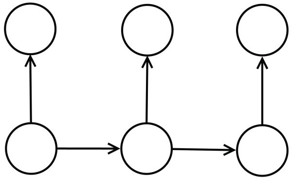
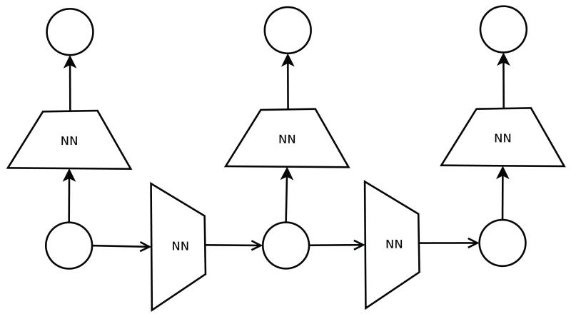
The starting point in this approach is a directed acyclic graph (DAG) associated with the data. Very often the DAG corresponds to a probabilistic graphical model (Bayesian network) of the data,46 although it does not have to be so. The directed edges typically correspond to causal or temporal relationships between the variables. For instance, in the case of sequence data, such as text data or biological sequence data, the graphs are often based on linear chains associated with Markov models (Figure 1), such as hidden Markov models (HMMS), input-output hidden Markov models, and other variants.47 With two dimensional data such as images, protein contact maps, or board games (e.g. GO), the graphs are typically based on two dimensional lattices with acyclic orientations. Other kinds of structured data may be associated with oriented trees. In all these cases, the DAG-RNN approach associates vector variables with the nodes of the DAG and places a neural network (or any other kind of parameterized function) on the edges of the DAG to parameterize the relationship between the corresponding vector variables. While a different network can be placed on each edge, when the DAG has a regular structure it is natural to share the weights of the neural networks associated with similar edges. For instance, in the example of Figures 1 and 2, the DAG associated with a hidden Markov model of the data can be converted to a deep neural network by using two basic neural network building blocks. One neural network for the transitions from state to state and one neural network for the emission of symbols from each state. These building blocks are shared or repeated at each position in time. When the architecture is unfolded in time or space, it yields a deep neural network with many layers and shared weights which can be trained by gradient descent (backpropagation) and other algorithms.
Figure 1.
Directed acyclic graph (DAG). This is the graphical model (Bayesian Network) representation of a first order Hidden Markov Model for sequence data. The HMM is defined by a finite set of hidden states, an alphabet of symbols, and two stochastic matrices: one for the state transitions, and one for the symbol emissions from a given state. Horizontal edges correspond to transitions between hidden (non visible states). Vertical edges correspond to emissions of symbols.
Figure 2.
Directed acyclic graphs recursive neural network (DAG-RNN). A feedforward neural network (or any other parameterized deterministic function) is assigned to each edge of the DAG. The neural network implements a deterministic function between corresponding input vectors and output vectors. The architecture and parameters of the neural networks can be shared across similar edges. In this case, this yields a model associated with two neural networks only: one to compute the next state vector given the current state vector, and one to compute the emitted symbol given the current state vector.
Undirected Graph Recursive Neural Networks (UG-RNN)
The DAG-RNN approach has been applied successfully to several problems, ranging for instance from protein secondary structure,43 to protein contact map44 prediction, to the game of GO.45 However it raises the obvious question of how it can be extended to domains where the graphs associated with the data are undirected graphs (UG) and possibly cyclic, which is obviously the case for small-molecule data. One possible approach is to try to convert the UG into a DAG in some canonical fashion. For small molecules one could use an approach similar to what is used to produce canonical SMILES strings to derive a canonical numbering of the vertices and thus a canonical orientation of the edges. However the resulting canonical orientation is likely to be quite arbitrary among all possible orientations, and hence unsatisfactory. Here instead we take an approach which finesses this problem essentially by taking all possible acyclic orientations into consideration and using them as an ensemble. This is possible here because small molecules have a relatively small number of nodes and edges and thus considering all possible acyclic orientations is computationally feasible. The process is schematically illustrated in Figures 3 and 4. Starting from an undirected graph, we cycle through all the vertices. When a given vertex is selected as the root, a DAG is generated by orienting all the edges towards the root along the shortest possible paths. Each DAG has the same vertices as the original UG, and essentially the same edges except that the edges are single oriented edges. In some cases, some of the original undirected edges can be oriented in either direction while leaving the overall derived graph acyclic. One possibility is to include all such possible orientations. Another possibility is to choose one orientation at random. Here, to keep things more manageable, we simply delete the corresponding ambiguous edges from the corresponding DAG. In short, if a molecular graph has N vertices associated with N atoms, this procedure yields N DAGs. We can then apply the DAG-RNN approach to each of the resulting DAGs and combine the outputs of all the DAG-RNN models to obtain an ensemble and derive a final prediction.
Figure 3.
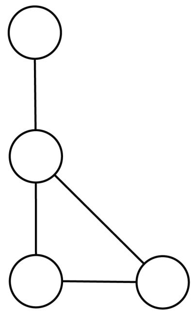
Undirected graph.
Figure 4.
Directed acyclic graphs.
More precisely consider a molecular graphs with N nodes v1, … , vN, and N associated DAGs derived by the process above. A “contextual” vector Gv,k is associated with each node v in each DAG indexed by k. This vector is a function of the local properties of the node v and of the contextual vectors associated with its parent nodes in the form:
| (2) |
where is the input vector associated with the properties of vertex v (e.g. information about the corresponding atom) and are the parents of vertex v in the kth DAG. Notice how this representation is recursive–each context vector is computed as a function of other context vectors. The function MG which implements this recursion by “crawling” the molecular graph is implemented by a parameterized neural network, although other classes of parameterized functions can also be used. The neural network is taken to be the same for all molecules, all DAGs, and all vertices. While this is not strictly necessary, for instance different NNs could be used for different classes of molecules, this strong weight sharing approach allows us to keep the number of free parameters in the model small. Notice how, in order for this representation to be possible, there must be an upper bound n to the number of parents a node can have (in the application presented in this work, typically n = 4). If a node has m parent nodes with m < n, blank vectors (all zeroes) are passed to the function MG as its last n–m arguments. Likewise, for a source node with no parents, only the input vector is non-zero: all the other components of the contextual vector are set to 0.
In this approach, one is free to choose the nature of the local information vector iv associated with each node v. This information could go well beyond the atom type and include, for instance, additional information about the local connectivity or properties of the molecule (e.g. aromaticity, topological indices, information about local paths or trees). To demonstrate the power of the UG-RNN approach and the underlying hypothesis that such information is extracted automatically by the crawling process, here we use only the atom type of the node and the bond type (single, double, triple) associated with the edges connecting the node to its parents . This information is encoded as a binary vector with one-hot encoding (e.g. with three atom types only, the atom type is encoded as: C=(1,0,0), N=(0,1,0), and O=(0,0,1) and similarly for the bond types).
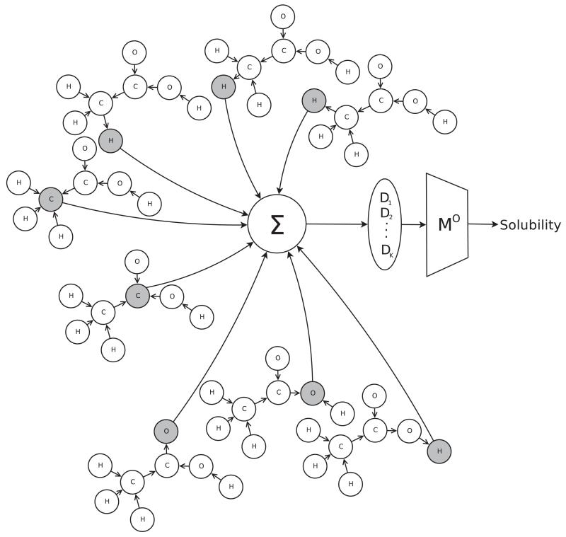
As there is a path from each atom in a DAG to the root of the DAG, the recursion above ends up producing a final contextual vector in the root node of each DAG which receives, directly or indirectly, some contribution from all the other contextual vectors in the DAG. Intuitively this vector can be viewed as the final product or summary of the crawling process in the corresponding DAG–it is a “view of the molecule” as seen from the corresponding root node. The N different views can be combined in different ways. Here we simply add the corresponding vectors. Thus, the overall description of the molecule is obtained as the sum of descriptions of the molecule “as seen” from each of its nodes/atoms. More formally, Gstructure is defined as:
| (3) |
where here rk denotes the root of the k-th DAG. Thus Gstructure can be viewed as a feature vector with K learnt features. The final prediction is produced by the output function MO
| (4) |
where p is a class probability in classification problems, or a continuous value in regression problem. Just like the encoding function MG, the output function MO can be implemented by a feed-forward neural network. An example of an alternative approach for combining the different views would be to apply a predictor to the contextual vector of each root node, and then take the average prediction of the ensemble. In either case, the resulting overall model is a deep feedforward neural network and therefore it can be trained by gradient descent.48-51 The feedforward nature is a direct consequence of the use of the DAGs in the encoding step. Given a set of training examples, the parameters of the MO and MG networks can be trained by gradient descent to minimize the error (e.g. squared error in the case of regression, relative entropy in the case of classification) between predicted and true values. Thus the features used to encode molecules are learnt by the system in a fully automated and task-specific manner. That is, if training is successful, the Gstructure vector provides an encoding of the molecular graph that is optimal in terms of minimizing the prediction error.
Example: UG-RNN Model of Acetic Acid
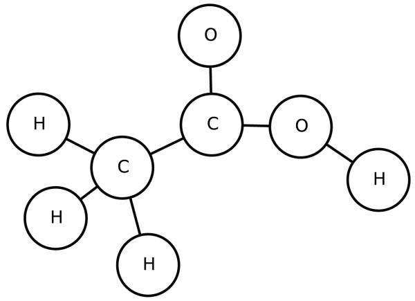
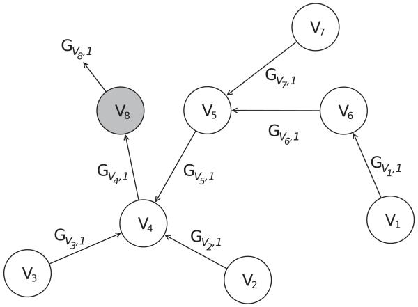
In this section, we illustrate the UG-RNN approach in detail using the acetic acid molecule (Figures 5 and 6) as a concrete example. For illustration purposes, we include hydrogen atoms but in practice these are implicit and can be omitted which has the advantage of leading to more compact architectures and faster training. In this case, the graph for acetic acid has eight nodes. The first step consists in generating the corresponding eight DAGs, each one with edges directed towards a different root node (Figure 7, root atoms highlighted). The second step consists in initializing the contextual vector for each source node and each DAG and then propagating the information along the DAG edges, using the neural network MG, to calculate the contextual vector for all the internal nodes, up to the root node. Specifically, using the top DAG in Figure 7 with root node v8 as the example, one must initialize the contextual vector for four source nodes: v1,v2,v3 associated with hydrogen atoms and v7 associated with an oxygen atom (Figure 8). For these four boundary nodes, the contextual vector of the parents is set to 0 and only the input vector associated with the vertex is set to a non-zero value, corresponding to the atom type. Information is then propagated along the DAG structure using Equation 2 and the current parameter values for the function MG to compute the contextual vector of each internal node, and ultimately of the root (sink node) v8, resulting in the vector Gv8,1 (Figure 8). The same procedure is applied to the other seven DAGs, finally producing eight vectors, each one describing the molecular structure “as seen” from the root of each DAG. The third step consists in generating the vector Gstructure describing the whole molecular graph by computing the sum of the eight contextual vectors associated with the eight roots of the eight DAGs (Figure 9). The fourth and final step consists in mapping the vector Gstructure using the output function MO into the property of interest, in this case aqueous solubility. During training, the error between the predicted and true value is computed for each training examples and the parameters of MG and MO are then adjusted by gradient descent.
Figure 5.
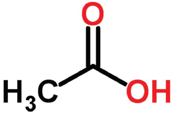
Acetic acid.
Figure 6.
Acetic acid undirected graph.
Figure 7.
Acetic acid DAGs.
Figure 8.
Application of MG to the first DAG.
Figure 9.
Sum of eight G vectors to produce the vector Gstructure = (D1, … , DK) corresponding to K descriptors learnt from the data. the output function MO produces the final prediction.
UG-RNN With Contracted Rings
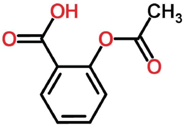
It is well known52,53 that backpropagation can run into problems of gradient diffusion or exploding or vanishing gradients in deep architectures, including recursive architectures and that, generally speaking, the severity of these problems tend to increase with the depth of the architectures. Thus here we consider also an approach which aims at reducing the depth of the recursive architectures essentially by contracting rings in molecular UGs to single points. Cyclic and polyciclic molecules with one or more rings are of course very common.54 An example of molecule with a single ring is Aspirin (Figure 10) and an example of polycyclic molecule is Amoxicillin (Figure 11).
Figure 10.
Aspirin.
Figure 11.
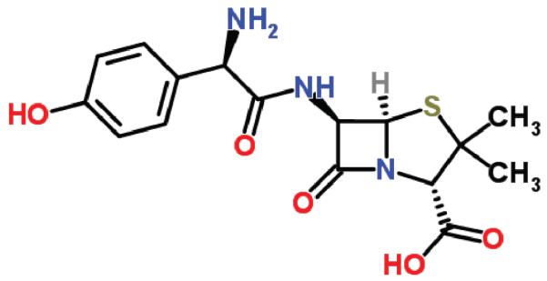
Amoxicillin.
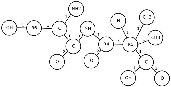
If one computes the Smallest Set of Smallest Rings55,56 of the molecular graph G and contracts each ring to a single node, one obtains a new undirected graph Gc with a smaller diameter than G. A new node representing a ring R is assigned a new label Rn where n is the length of the ring, capped to the length of the largest ring in the data. The new node is connected to all the non-ring nodes that were originally connected to the ring R, with edge type labels equal to those of the original bonds. In addition, for polyciclic molecules, a new node associated with a ring R can also be connected to other newly created nodes that are associated with rings sharing at least one vertex with R. Although we experimented with various edge labeling rules, in the end using the same label as for single-bond edges for all new edges arising between such newly created nodes provides the most simple and effective solution.
Applying this procedure to the graphs representing Aspirin and Amoxicillin yields the graphs in Figures 12 and 13, respectively. Thus in the experiments we explore also an alternative approach in which the graph representing a molecule is first reduced by contracting its rings using the procedure above, and then the UG-RNN approach is applied. We call this approach UG-RNN with Contracted Rings (UG-RNN-CR).
Figure 12.
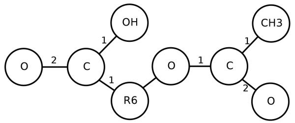
Contracted graph of Aspirin with bond types.
Figure 13.
Contracted graph of Amoxicillin with bond types.
Data
To train and test the approach we use four publicly available benchmark datasets widely used in the solubility prediction literature.
Small Delaney Dataset
This dataset15 originally contained 2874 molecules together with their measured aqueous solubility (logmol/L at 25 °C). This dataset is particularly interesting because it can be used as a benchmark for comparisons against the GSE method.23 As described in Delaney,15 the GSE was obtained from a set of molecules similar to the ones contained in the “Small” Delaney Dataset. Furthermore, various kernel methods57 have also been trained and tested on this dataset with better results than GSE.
Huuskonen
This dataset contains 1026 organic molecules selected by Jarmo Huuskonen58 from the AQUASOL dATAbASE59 and the PHYSPROP Database.60 Molecules are listed together with their aqueous solubility values, expressed in logmol/L at 20-25°. For instance, Frohlich et al.61 report a squared correlation coefficient of 0.90 for an 8-fold cross-validation, using support vector machines with a RBF (Radial Basis Function) kernel.
Intrinsic Solubility Dataset
This dataset contains 74 molecules together with their intrinsic solubility values reported by Bergstrom62,63 and others.23,64,65 The dataset has been selected by Louis et al.,25 to test a wide range of predictive methods, including linear models, SVMs, and shallow Neural Networks. Because of its small size, this set is useful for assessing the performances of the UG-RNN method when its training set contains few input/output examples.
Solubility Challenge Dataset
This dataset contains 125 molecules selected by Linas et al.66 using the criteria that molecules ought to contain a ionizable group (pKa between 1-13) and be commercially available. The set is divided into two subsets: a training set containing 97 molecules, and a test set containing 28 molecules. The challenge consisted in predicting the solubility of the molecules in the test set using the solubility values of the molecules in the training set.
In general, we use 10-fold cross validation methods to assess the performance of the various UG-RNN predictors. Thus we divide the data randomly into 10 subsets of equal size, and use nine of them for training and the remaining one for testing, in all 10 possible combinations. We then compute the average and standard deviation of the performance across the ten data splits. In addition each training set, consisting of 90% of the original data, is randomly split into a proper training set and a small validation set using an 80/20 proportion for the datasets containing more than 1000 examples (Delaney and Huuskonen), and an 85/15 proportion for the smaller datasets (Intrinsic Solubility and Solubility Challenge Datasets). The validation set is used to fit the hyperparameters of the models (see below). The different proportions are used to match what is reported in the literature for comparison purposes. The details of all the dataset splits are given in supplementary information.
Additional Methodological Aspects
As previously mentioned, both the encoding function MG and the output mapping function MO are implemented using a neural network. In both cases, we use a standard three-layer neural network architecture, with one hidden layer. All neurons use a sigmoid transfer function (tanh) and weights are randomly initialized. In order to reduce the residual generalization error,67 we use an ensemble of 20 models with a different number of hidden units and features (i.e. the outputs units of MG), as described in Table 1. The optimal value of the learning rate η is determined by varying it from 10−1 to 10−4 and keeping the value which gives the lowest RMSE (Root Mean Square Error) (see Metrics). To facilitate learning, we slightly modify the gradient descent procedure as in.50,51 Specifically, the gradient of the error with respect to a weight dw is used to modify the weight according to the simple gradient descent rule Δw = −ηdw only if |dw| ∈ [0.1,1]. Outside this range, to avoid exploding or vanishing gradients, the learning rule is clipped: Δw = −ηsign(dw) if |dw| > 1, or Δw = −η0.1sign(dw) if |dw| < 0.1. Each UG-RNN model is trained for 5000 epochs and the outputs of the best 10 networks, selected by their Root Mean Square Error (RMSE) on the validation set, are averaged as an ensemble to compute the prediction on the test set, during each fold of the 10-fold cross validation procedure.
Table 1.
Architecture of 20 encoding neural networks MG and output neural networks MO
| NeuralNetwork |
MG Hidden Units |
MG Output Units |
MO Hidden Units |
|---|---|---|---|
| Model_1 | 7 | 3 | 5 |
| Model_2 | 7 | 4 | 5 |
| Model_3 | 7 | 5 | 5 |
| Model_4 | 7 | 6 | 5 |
| Model_5 | 7 | 7 | 5 |
| Model_6 | 7 | 8 | 5 |
| Model_7 | 7 | 9 | 5 |
| Model_8 | 7 | 10 | 5 |
| Model_9 | 7 | 11 | 5 |
| Model_10 | 7 | 12 | 5 |
| Model_11 | 3 | 3 | 5 |
| Model_12 | 4 | 3 | 5 |
| Model_13 | 5 | 3 | 5 |
| Model_14 | 6 | 3 | 5 |
| Model_15 | 7 | 3 | 5 |
| Model_16 | 8 | 3 | 5 |
| Model_17 | 9 | 3 | 5 |
| Model_18 | 10 | 3 | 5 |
| Model_19 | 11 | 3 | 5 |
| Model_20 | 12 | 3 | 5 |
Because of the importance given to the octanol-water partition coefficient in the aqueous solubility literature, we also assess the performances of both the UG-RNN model and the UG-RNN-CR model using two different inputs for the output network MO. In addition to the case described above where the input to MO is the vector Gstructure alone, we also consider the case where the input consists of Gstructure plus the logPoctanol (calculated using Marvin Beans68). In this way, we can partially assess how logPoctanol affects the generalization capability of the UG-RNN and UG-RNN-CR models and better understand the kind of information contained in the vector Gstructure.
Results
Metrics
In order to assess the performance of the UG-RNN predictors and compare them with other methods, we use three standard metrics: the root mean square error (RMSE), the average absolute error (AAE), and the Pearson correlation coefficient (R) defined by
| (5) |
| (6) |
| (7) |
Here pi is the predicted value and ti is the target value (experimentally observed) for molecule i. In some cases, we use R2 instead of R as our error metric in order to compare our results with other published results. In the tables, for clarity purposes the best results are marked in bold.
Small Delaney Dataset
Results obtained by 10-fold cross validation on the Small Delaney Dataset are shown in Table 2. The UG-RNN approach gives the best results for every metric and the UG-RNN-CR’ approach does not perform as well. Including the logP information leads to significant improvements for the simplified UG-RNN-CR approach with contracted rings, but not for the full UG-RNN approach with no ring contractions. The best UG-RNN models match or surpass the perfomances of the GSE and 2D Kernel methods, although generally the differences are within one standard deviation.
Table 2.
Prediction performances and standard deviations using 10-fold cross validation on the Small Delaney Dataset (1144 molecules)
Huuskonen Dataset
Results obtained by 10-fold cross validation on the Huuskonen Dataset are shown in Table 3 and are consistent with those observed on the Small Delaney dataset. The UG-RNN method achieves the best results for all the metrics. Adding the logP information does not improve its performance, but significantly improves the performance of the restricted UG-RNN-CR method with contracted rings. Published performances obtained with kernel methods are similar to the performance of the UG-RNN models.
Table 3.
Prediction performances and standard deviations using 10-fold cross validation on the Huuskonen Dataset (1026 molecules)
| Models | R 2 | std R2 | RMSE | std RMSE | AAE | sdt AAE |
|---|---|---|---|---|---|---|
| UG-RNN | 0.91 | 0.01 | 0.60 | 0.06 | 0.46 | 0.04 |
| UG-RNN-CR | 0.80 | 0.04 | 0.92 | 0.07 | 0.65 | 0.05 |
| UGR-NN+LogP | 0.91 | 0.01 | 0.61 | 0.06 | 0.47 | 0.04 |
| UG-RNN-CR+LogP | 0.89 | 0.02 | 0.68 | 0.06 | 0.52 | 0.04 |
| RBF Kernel61 | 0.90 | - | - | - | - | - |
Intrinsic Solubility Dataset
Results obtained by 10-fold cross validation on the Intrinsic Solubility Dataset are shown in Table 4. On this small dataset, the best performing model is UG-RNN-CR+logP across all three metrics used. The UG-RNN model does not seem to be able to generalize well on this dataset, probably because of its small size (only 60 training examples). UG-RNN-CR does not perform well but it benefits substantially from the inclusion of logP in the input label. In fact, UG-RNN-CR+logP is the only UG-RNN-based method to outperform the best method by Louis et al.25 The latter is based on a feed forward neural network whose input layer consists of a set of four descriptors: logP and three topological descriptors 1χV, Δ2χ and 2IC. Given that in the UG-RNN-CR+logP the mapping function is also implemented by a feedforward neural network with logP as one of the inputs, the only substantive difference between the two approaches is the choice of the other input features. These are chosen in advance and “hand-crafted” in the previously published approach, whereas they are automatically learnt from the data in the UG-RNN approach.
Table 4.
Prediction performances and standard deviations using 10-fold cross validation on the Intrinsic Solubility Dataset (74 molecules)
| Models | R | std R | RMSE | sdt RMSE | AAE | std AAE |
|---|---|---|---|---|---|---|
| UG-RNN | 0.64 | 0.04 | 0.96 | 0.01 | 0.80 | 0.11 |
| UG-RNN-CR | 0.55 | 0.09 | 1.05 | 0.12 | 0.88 | 0.12 |
| UG-RNN+LogP | 0.67 | 0.02 | 0.93 | 0.07 | 0.77 | 0.06 |
| UG-RNN-CR+LogP | 0.81 | 0.01 | 0.72 | 0.04 | 0.51 | 0.03 |
| Louis et al.25 | 0.74 | - | 0.73 | - | 0.53 | - |
Solubility Challenge Dataset
Results obtained by 10-fold cross validation on the Solublity Challenge Dataset are shown in Table 5. On this dataset, we provide a comparison with the relevant work of Hewitt et al.11 assessing the predictive performances of three different approaches: linear regression, artificial neural networks, and category formation. The input for their models was a vector consisting of 426 molecular descriptor values, computed using the Dragon Professional software (Version 5.3).69 For validation purposes, the molecules in the training set were ordered according to their solubility values and every fifth molecule was taken as a validation molecule. Furthermore, a genetic algorithm approach was used to select the molecular descriptors providing the best predictive performance on the validation set. For completeness, they also applied several commercially available solubility predictors to the Solubility Challenge test set. Perhaps surprisingly, they observed that: a simple Multiple Linear Regression method (MLR-Sol-Chal) obtained better results than a more complex approach based on Neural Networks (NN-Sol-Chal); commercially available tools, trained on bigger datasets, obtained better results than MLR-Sol-Chal, but not as good as expected.
Table 5.
Prediction performance and standard deviations using 10- fold cross validation on the Solubility Challenge Dataset (125 molecules)
| Models | R 2 | std R2 | RMSE | std RMSE | AAE | std AAE |
|---|---|---|---|---|---|---|
| UG-RNN | 0.32 | 0.03 | 1.41 | 0.12 | 1.08 | 0.10 |
| UG-RNN-LogP | 0.45 | 0.04 | 1.27 | 0.13 | 1.03 | 0.11 |
| UG-RNN-CR-LogP | 0.44 | 0.09 | 1.28 | 0.18 | 1.03 | 0.16 |
| UG-RNN-Huusk | 0.43 | 0.02 | 1.16 | 0.03 | 0.93 | 0.03 |
| UG-RNN-Huusk-Sub | 0.48 | 0.02 | 1.11 | 0.03 | 0.84 | 0.01 |
| UG-RNN-LogP-Huusk | 0.54 | 0.02 | 1.00 | 0.03 | 0.82 | 0.03 |
| UG-RNN-LogP-Huusk-Sub | 0.60 | 0.02 | 0.94 | 0.02 | 0.71 | 0.02 |
| UG-RNN-CR-LogP-Huusk | 0.62 | 0.03 | 0.96 | 0.06 | 0.83 | 0.06 |
| UG-RNN-CR-LogP-Huusk-Sub | 0.67 | 0.03 | 0.90 | 0.06 | 0.74 | 0.05 |
| NN-Sol-Chal11 | 0.40 | - | 1.51 | - | - | - |
| MLR-Sol-Chal11 | 0.51 | - | 0.95 | - | 0.77 | - |
| New in silico consesus11 | 0.60 | - | 0.90 | - | 0.68 | - |
The UG-RNN models are trained using the Solubility Challenge training set and we observe that the best performing models (UGRNN-LogP and UGRNN-CR-LogP) obtain worse results than MLR-Sol-Chal, but better results than the neural-network-based (NN-Sol-Chal). The fact that the UG-RNN-based models outperform the NN-Sol-Chal model provides evidence that the automated feature selection of the UG-RNN method can capture molecular properties which are more informative for the task at hand than pre-computed molecular descriptors. We also observe large standard deviations on each metric, indicating that there is considerable variability in the results across different folds. Such variability is a sign of overfitting, and, as already suggested by Hewitt at al., this is a clear sign that the training set is too small and does not contain enough information to address the solubility problem with any kind of generality. Moreover, the average Tanimoto similarity of each molecule in the test set to its ten closest neighbors in the training set is only 0.53, which also suggests that at least some of the molecules in the test set are likely to be outside the applicability domain of the trained models.
Thus one may suspect that larger training sets could lead to significant performance improvements. To test this hypothesis, we also train several UG-RNN-based models on an expanded training set that includes the molecules from both the Solubility Challenge Dataset and the Huuskonen Dataset. Since the training set should not contain any molecule that is present in the test set, we must remove all shared molecules. Therefore, before starting the training procedure, we compute all the pairwise Tanimoto similarities between the molecules in the Huuskonen dataset and the Solubility Challenge test set. We find that the two datasets share 10 molecules and some of the shared molecules are assigned significantly different log solubility values (6). Perhaps the most striking and controversial discrepancy is provided by indomethacin, which is known to be practically insoluble in water.70 It is reported to have a solubility value of −2.94 log units in the Solubility Challenge Dataset to be contrasted with a value of −4.62 in the Huuskonen Dataset, a difference of more than 1.5 log units. We also noticed differences in excess of 0.5 log units for hydrochlorothiazide and dibucaine. The method adopted to determine experimental solubility values (Chasing Equilibrium) for the Solubility Challenge is supposed to ensure a log error of 0.05 units,66 however the significant discrepancies with some of the values reported in the literature casts some doubts.11 In any case, in 5, we also report the performance of the UG-RNN-based models when the solubility values of the Solubility Challenge test set are replaced with the solubility values of the Huuskonen dataset (only for the shared molecules). As expected, expansion of the training set results in significant performance improvement for all the metrics, as well as shrinking of the standard deviations. In particular, the UG-RNN-CR-LogP-Huusk model obtains an average squared correlation R2 = 0.67 that is even better than the one reported in Hewitt et al. (R2 = 0.62) obtained with an ensemble of commercial solubility tools (the new in silico consensus). Furthermore, it is interesting to note that the substitution of the Huuskonen solubility values further improves the overall performance of the UG-RNN-based models, with UG-RNN-CR-LogP-Huusk performing the best, with an average squared correlation R2 = 0.67.
In summary, the results obtained across all four datasets are quite consistent in demonstrating the general effectiveness and competitiveness of the UG-RNN approach in its different forms while also exposing the fundamental problems arising from training sets that are too small or too noisy.
Domain of Applicability
Estimating the domain of applicability (DOA) of a QSAR model is essential to obtain reliable predictions. Schröter et al,71 for instance, state that predictions of aqueous solubility for molecules whose structure falls outside the DOA are generally poor. In the literature there are several methods to estimate the DOA of a QSAR model. It is possible to sort them into three categories: range-based methods,72-74 distance-based methods,72-75 and probability-distribution- based methods.72 Here we employ a distance-based method using Euclidean distance to estimate the DOA of the UG-RNN trained on the Small Delaney Dataset.15 For completeness, we also use the Tanimoto similarity measure.
During training, as described in the data section, this dataset is randomly partitioned into 10 folds, yielding for each round of cross-validation a test set containing 10% of the entire dataset (i.e. 115 molecules) and a training set containing the remaining 90%. In addition, 20% of each training set is set aside for validation purposes, leaving in effect 10 training sets containing 78% of the entire dataset (i.e. 823 molecules). To estimate the DOA, for each of the 10 selected models, we first compute the Euclidean distance between each molecule i in a test set and each molecule j in the corresponding training set by
| (8) |
where K is the length of the encoding vectors produced by the first stage of the UG-RNN method. We then compute the average distance Di for each molecule i in a test set to the corresponding training set by
| (9) |
where here T denotes the number of molecules in the corresponding training set. When this calculation is applied to each fold, one ends up with an average distance di for each molecule in the entire dataset, and for each one of the 10 selected models. A similar procedure is carried also with other metrics, such as the Tanimoto similarity measure, computed for each molecule by taking the average similarity to its 10 most similar neighbors in the corresponding training set, using the FP4 Open Babel fingerprint format (http://openbabel.org/wiki/Tutorial:Fingerprints).
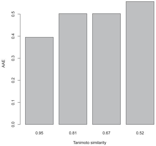
The next step consists in binning the data according to di into bins of equal size and calculating the average absolute error AAEb for each bin b
| (10) |
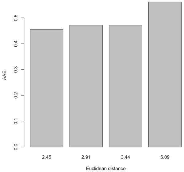
where B is the number of molecules in each bin. The results are shown in Figure 14 with corresponding Table 7 for the Euclidean distance, and in Figure 15 with the corresponding Table 8 for the Tanimoto similarity. In both cases, we use four bins of equal size. One can clearly observe that on average prediction errors increase with distance or dissimilarity, albeit not linearly. Therefore, making predictions only for molecules which have an average distance or dissimilarity from the training set below a certain threshold (e.g. 2.45 ± 0.15 in Euclidean distance) could be a way to improve the reliability of the predictor in a screening pipeline, in the absence of larger and more diverse training sets.
Figure 14.
Relationship between Euclidean distances and average absolute error using four bins.
Table 7.
AAE, average Euclidean distance, and standard deviation. Each bin contains 2860 distances.
| Bin Number | 1 | 2 | 3 | 4 |
|---|---|---|---|---|
| AAE | 0.45 | 0.47 | 0.48 | 0.56 |
| distance (av) | 2.45 | 2.91 | 3.44 | 5.09 |
| distance (st dev) | 0.15 | 0.14 | 0.18 | 1.67 |
Figure 15.
Relationship between Tanimoto similarity values and average absolute error using four bins.
Table 8.
AAE, average Tanimoto similarity, and standard deviation. Each bin contains 2860 similarity measures.
| Bin Number | 1 | 2 | 3 | 4 |
|---|---|---|---|---|
| AAE | 0.40 | 0.50 | 0.51 | 0.56 |
| similarity (av) | 0.95 | 0.81 | 0.67 | 0.52 |
| similarity (st dev) | 0.05 | 0.04 | 0.04 | 0.08 |
Training Time
The training time for the UG-RNN models scales roughly linearly with the size of the training set and with the diameter of the molecules being processed. Detailed training times are given in supplementary information but for the data considered here the average time per molecule and per epoch is 7.8 milliseconds on a good workstation. Thus the training time is quite reasonable and much larger datasets could be accommodated by this method. The approach could be further accelerated by using GPUs or parallel distributed implementations if necessary.
Internal Representations
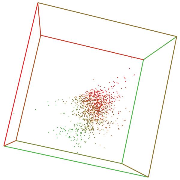
Figure 16 shows the 3D space arrangement of the UG-RNN feature vectors Gstructure resulting from a training process on the Small Delaney dataset. In this case, we use a small network with K = 3 in order to enforce low-dimensional, easy-to-visualize, feature vectors. Each point correspond to the image of a molecular structure in the space of features. The color of the point, scaled from green to red, represents the aqueous solubility of the corresponding molecule. One can notice immediately that points with the same color tend to be colocated in the 3D plot. This illustrates how the internal representation of molecular structures learnt by the UG-RNN models can be correlated with the task at hand, providing further evidence of their capability to automatically extract from the molecular graphs features that are relevant for the prediction of a given property.
Figure 16.
Scatter plot of learnt feature vectors for molecules in the Small Delaney dataset.
Conclusion
Experimental results show that the UG-RNN approach can be used to build aqueous solubility predictors that match and sometimes outperform current state-of-the-art methods. One important difference between UG-RNN-based approaches with respect to other methods, is the ability to automatically extract internal representations from the molecular graphs that are well suited for the specific tasks. This aspect is an important advantage for a problem like aqueous solubility prediction, where the optimal feature set is not known and may even vary from one dataset to the other. It also saves time and avoids other costs and limitations associated with the use of human expertise to select features.
The UG-RNN standard model performs well on both the Small Delaney dataset and the Huuskonen datasets, while its results on the Intrinsic Solubility dataset are weaker. A likely explanation for this observation is the particularly small size of the Intrinsic Solubility dataset which leads to overfitting and poor generalization. Moreover, the UG-RNN model does not seem to benefit from the addition of logP information to its set of features, a sign that the logP information is already implicitly contained in the learnt features.
The UG-RNN-CR model with contracted rings has weaker predictive capabilities on all the datasets used in this study. This suggests that the loss of information about ring structures negatively affects the generalization capability of the UG-RNN in spite of the decrease in the depth of the recursions which facilitates gradient propagation during learning. On the other hand, the model seems to be rescued when the logP information is added to its features (UG-RNN-CR+logP) providing further evidence that this information is implicitly extracted by the UG-RNN approach.
Finally, a UG-RNN-based web server for aqueous solubility prediction called AquaSol is available through the ChemDB chemoinformatics portal (cdb.ics.uci.edu) together with downloadable code and other information. However, the domain of applicability of predictors trained on a few hundreds or a few thousands of molecules is bound to be limited in chemical space and thus annotating and gathering larger datasets on aqueous solubility or other properties is important for future applications. This is why the main contribution of this paper is not the development of a specific predictor, but rather the development of a general deep learning methodology for chemoinformatics problems. The approach uses recursive neural networks adapted to undirected graphs representing molecular structures. A similar deep learning approach could be used also for other molecular representations. For instance, for 1D fingerprint representations, convolutional architectures could be used. For 2D representations based on adjacency matrices, the same 2D-RNN approaches51 used for protein contact map prediction could be used, as well as their more recent descendants.34,76 For 3D representations based on atom coordinates, local coordinate information, such as bond lengths and bond angles, could be included in the inputs of the neural networks used for this study. Similar ideas could also be applied to problems involving more than one molecule, for instance to predict molecular interactions or reaction grammars.6,7 It is precisely with growing amounts of freely available data and computing power that one can expect deep learning methods to become useful in different areas of chemoinformatics.
Supplementary Material
Table 6.
Differences in solubility values between the Solubility Challenge and the Huuskonen Datasets
| SMILES | Sol Chal | Huusk |
|---|---|---|
| CCN(CC)CCNC(C1=C(C=CC=C2)C2=NC(OCCCC)=C1)=O | −4.39 | −3.70 |
| CC/C(C1=CC=C(O)C=C1)=C(C2=CC=C(O)C=C2)/CC | −4.43 | −4.35 |
| O=S1(C2=CC(S(N)(=O)=O)=C(Cl)C=C2NCN1)=O | −3.68 | −2.62 |
| CN(C)CCCN1C2=C(C=CC=C2)CCC3=C1C=CC=C3 | −4.11 | −4.19 |
| COC1=CC=C2C(C(CC(O)=O)=C(C)N2C(C3=CC=C(Cl)C=C3)=O)=C1 | −2.94 | −4.62 |
| CCN(CC)CC(NC1=C(C)C=CC=C1C)=O | −1.87 | −1.76 |
| NC1=CC=C(S(NC2=NC(C)=CC=N2)(=O)=O)C=C1 | −3.12 | −2.85 |
| CC1=CC=C(S(NC(NCCCC)=O)(=O)=O)C=C1 | −3.46 | −3.39 |
Acknowledgement
AL is funded through a GREP Ph.D. scholarship from the Irish Research Council for Science, Engineering and Technology. GP’s research is funded through SFI grant 10/RFP/GEN2749. PB’s research is supported by the following grants: NSF IIS-0513376, NIH LM010235, and NIH NLM T15 LM07443. We wish to acknowledge OpenEye Scientific Software and ChemAxon for academic software licenses, and Jordan Hayes and Yuzo Kanomata for computing support.
References
- (1).Scholkopf B, Smola AJ. Learning with Kernels. MIT Press; Cambridge, MA: 2002. [Google Scholar]
- (2).Ralaivola L, Swamidass SJ, Saigo H, Baldi P. Neural Networks. 2005;18:1093, 1110. doi: 10.1016/j.neunet.2005.07.009. Special issue on Neural Networks and Kernel Methods for Structured Domains. In press. [DOI] [PubMed] [Google Scholar]
- (3).Azencott C, Ksikes A, Swamidass SJ, Chen J, Ralaivola L, Baldi P. Journal of Chemical Information and Modeling. 2007;47:965–974. doi: 10.1021/ci600397p. [DOI] [PubMed] [Google Scholar]
- (4).Ceroni A, Costa F, Frasconi P. Bioinformatics. 2007;23:2038–2045. doi: 10.1093/bioinformatics/btm298. [DOI] [PubMed] [Google Scholar]
- (5).Mahé P, Vert J-P. Machine learning. 2009;75:3–35. [Google Scholar]
- (6).Kayala M, Azencott C, Chen J, Baldi P. Journal of Chemical Information and Modeling. 2011;51:2209–2222. doi: 10.1021/ci200207y. [DOI] [PMC free article] [PubMed] [Google Scholar]
- (7).Kayala M, Baldi P. Journal of Chemical Information and Modeling. 2012;52:2526–2540. doi: 10.1021/ci3003039. [DOI] [PubMed] [Google Scholar]
- (8).Waterbeemd HVD, Gifford E. Nature Reviews. 2003;2:192–204. doi: 10.1038/nrd1032. [DOI] [PubMed] [Google Scholar]
- (9).Starita A, Micheli A, Sperduti A. J. Chem. Inf. Comput. Sci. 2000;41:202–218. doi: 10.1021/ci9903399. [DOI] [PubMed] [Google Scholar]
- (10).Fühner H. Ber. Dtsch. Chem. Ges. 1924;57B:510–515. [Google Scholar]
- (11).Hewitt M, Cronin MTD, Enoch SJ, Madden JC, Roberts DW, Dearden JC. J. Chem. Inf. Model. 2009;49:2572–2587. doi: 10.1021/ci900286s. [DOI] [PubMed] [Google Scholar]
- (12).Reynolds J, Gilbert DB, Tanford C. Proc. Natl. Acad. Sci. 1974;71:2925–2927. doi: 10.1073/pnas.71.8.2925. [DOI] [PMC free article] [PubMed] [Google Scholar]
- (13).Hansch C, Quinlan JE, Lawrence GL. J. Org. Chem. 1968;33:347–350. [Google Scholar]
- (14).Faller B, Ertl P. AdV. Drug DeliVery ReV. 2007;59:533–545. doi: 10.1016/j.addr.2007.05.005. [DOI] [PubMed] [Google Scholar]
- (15).Delaney JS. J. Chem. Inf. Comput. Sci. 2003;44:1000–1005. doi: 10.1021/ci034243x. [DOI] [PubMed] [Google Scholar]
- (16).Yalkowsky SH, Valvani SC. J. Pharm. Sci. 1980;69:912–922. doi: 10.1002/jps.2600690814. [DOI] [PubMed] [Google Scholar]
- (17).Kamlet MJ, Doherty RM, Abboud J-LM, Abraham MH, Taft RW. J. Pharm. Sci. 75:338–348. 1986. doi: 10.1002/jps.2600750405. [DOI] [PubMed] [Google Scholar]
- (18).Randic M. J. Am. Chem. Soc. 1975;97:6609–6615. [Google Scholar]
- (19).Kier LB, Hall LH. Academic Press; New York: 1976. Molecular ConnectiVity in Chemistry and Drug Design. [Google Scholar]
- (20).Kier LB, Hall LH. Molecular ConnectiVity in Structure-ActiVity Analysis. John Wiley & Sons; New York: 1986. [Google Scholar]
- (21).Leo A, Hansch C, Elkins D. Chemical Reviews. 1971;71:525–616. [Google Scholar]
- (22).Leo A. Chemical Reviews. 1993:1281–1306. [Google Scholar]
- (23).Jain N, Yalkowsky S. J. Pharm. Sci. 2001;90:234–252. doi: 10.1002/1520-6017(200102)90:2<234::aid-jps14>3.0.co;2-v. [DOI] [PubMed] [Google Scholar]
- (24).Timmerman H, Todeschini R, Consonni V, Mannhold R, Kubiny H. Handbook of Molecular Descriptors. Wiley-VCH; Weinheim: 2002. [Google Scholar]
- (25).Louis B, Agrawal VK, Khadikar PV. European Journal of Medicinal Chemistry. 2010;45:4018–4025. doi: 10.1016/j.ejmech.2010.05.059. [DOI] [PubMed] [Google Scholar]
- (26).Dearden J. Expert Opinion in Drug DiscoVery. 2006;1:31–52. doi: 10.1517/17460441.1.1.31. [DOI] [PubMed] [Google Scholar]
- (27).Dannenfelser RM, Paric M, White M, Yalkowsky S. Chemosphere. 1991;23(2):141–165. [Google Scholar]
- (28).Jorgensen W, Duffy E. Adv. Drug Del. Rev. 2002;54(30):355–366. doi: 10.1016/s0169-409x(02)00008-x. [DOI] [PubMed] [Google Scholar]
- (29).Hinton G, Osindero S, Teh Y. Neural Computation. 2006;18:1527–1554. doi: 10.1162/neco.2006.18.7.1527. [DOI] [PubMed] [Google Scholar]
- (30).Bengio Y, LeCun Y. Scaling learning algorithms towards AI. 2007 [Google Scholar]
- (31).Lee H, Grosse R, Ranganath R, Ng A. Convolutional deep belief networks for scalable unsupervised learning of hierarchical representations. 2009 [Google Scholar]
- (32).Lee H, Pham P, Largman Y, Ng A. Bengio Y, Schuurmans D, Lafferty J, Williams CKI, Culotta A, editors. Advances in Neural Information Processing Systems. 2009;22:1096–1104. [Google Scholar]
- (33).Hinton G, Srivastava N, Krizhevsky A, Sutskever I, Salakhutdinov RR. 2012 http://arxiv.org/abs/1207.0580. [Google Scholar]
- (34).Di Lena P, Nagata K, Baldi P. Bioinformatics. 2012;28:2449–2457. doi: 10.1093/bioinformatics/bts475. doi: 10.1093/bioinformatics/bts475. First published online: July 30, 2012. [DOI] [PMC free article] [PubMed] [Google Scholar]
- (35).Krizhevsky A, Sutskever I, Hinton G. Advances in Neural Information Processing Systems. 2012;25 [Google Scholar]
- (36).Socher R, Pennington J, Huang EH, Ng AY, Manning CD. Semi-Supervised Recursive Autoencoders for Predicting Sentiment Distributions. 2011 [Google Scholar]
- (37).Hinton G, Salakhutdinov R. Science. 2006;313:504. doi: 10.1126/science.1127647. [DOI] [PubMed] [Google Scholar]
- (38).Bengio Y, Lamblin P, Popovici D, Larochelle H, Montreal U. Advances in neural information processing systems. 2007;19:153. [Google Scholar]
- (39).Erhan D, Bengio Y, Courville A, Manzagol P-A, Vincent P, Bengio S. Journal of Machine Learning Research. 2010;11:625–660. [Google Scholar]
- (40).Baldi P. Designs, Codes, and Cryptography. 2012;65:383–403. [Google Scholar]
- (41).LeCun Y, Matan O, Boser B, Denker JS, Henderson D, Howard RE, Hubbard W, Jackel LD, Baird HS. Handwritten Zip Code Recognition with Multilayer Networks. 1990 invited paper. [Google Scholar]
- (42).LeCun Y, Bottou L, Bengio Y, Haffner P. Proceedings of the IEEE. 1998;86:2278–2324. [Google Scholar]
- (43).Baldi P, Brunak S, Frasconi P, Pollastri G, Soda G. Bioinformatics. 1999;15:937–946. doi: 10.1093/bioinformatics/15.11.937. [DOI] [PubMed] [Google Scholar]
- (44).Baldi P, Pollastri G. Journal of Machine Learning Research. 2003;4:575–602. [Google Scholar]
- (45).Wu L, Baldi P. Neural Networks. 2008;21:1392–1400. doi: 10.1016/j.neunet.2008.02.002. [DOI] [PubMed] [Google Scholar]
- (46).Koller D, Friedman N. Probabilistic Graphical Models: Principles and Techniques [Google Scholar]
- (47).Baldi P, Brunak S. Bioinformatics: the machine learning approach. Second edition MIT Press; Cambridge, MA: 2001. [Google Scholar]
- (48).Rumelhart DE, Hinton GE, Williams RJ. Nature. 1986;323:533–536. [Google Scholar]
- (49).Baldi P. IEEE Transactions on Neural Networks. 1995;6:182–195. doi: 10.1109/72.363438. [DOI] [PubMed] [Google Scholar]
- (50).Pollastri G, Baldi P. Bioinformatics. 2002;18:62, 70. doi: 10.1093/bioinformatics/18.suppl_1.s62. [DOI] [PubMed] [Google Scholar]
- (51).Baldi P, Pollastri G. Journal of Machine Learning Research. 2003;4:575–602. [Google Scholar]
- (52).Bengio Y, Simard P, Frasconi P. IEEE Transactions in Neural Networks. 1994;5(2):157–166. doi: 10.1109/72.279181. [DOI] [PubMed] [Google Scholar]
- (53).Larochelle H, Bengio Y, Louradour J, Lamblin P. The Journal of Machine Learning Research. 2009;10:1–40. [Google Scholar]
- (54).March J. Advanced Organic Chemistry: Reactions, Mechanisms, and Structure. 3rd ed. Wiley; New York: 1985. [Google Scholar]
- (55).Zamora A. Journal of Chemical Information and Computer Sciences. 1976;16:40–43. [Google Scholar]
- (56).Fan BT, Panaye A, Doucet JP, Barbu A. Journal of chemical information and computer sciences. 1993;33:657–662. doi: 10.1021/ci000004n. [DOI] [PubMed] [Google Scholar]
- (57).Azencott C-A, Ksikes A, Swamidass SJ, Chen JH, Ralaivola L, Baldi P. J. Chem. Inf. Comput. Sci. 2007;47:965–974. doi: 10.1021/ci600397p. [DOI] [PubMed] [Google Scholar]
- (58).Huuskonen J. J. Chem. Inf. Comput. Sci. 2000;40:773–777. doi: 10.1021/ci9901338. [DOI] [PubMed] [Google Scholar]
- (59).Yalkowsky SH, M. DR. The ARIZONA dATAbASE of Aqueous Solubility. College of Pharmacy, University of Arizona; Tucson, AZ: 1990. [Google Scholar]
- (60).Corporation . S. R. Physical/Chemical Property Database(PHYSOPROP) SRC Environmental Science Center; Syracuse, NY: 1994. [Google Scholar]
- (61).Fröhlich H, Wegner JK, Zell A. QSAR & Combinatorial Science. 2004;23:311–318. [Google Scholar]
- (62).Bergstroem C, Strafford M, Lazorova L, Avdeef A, Luthman K, Artursson P. J. Med. Chem. 2003;46:558–570. doi: 10.1021/jm020986i. [DOI] [PubMed] [Google Scholar]
- (63).Wassvik C, Holmen A, Bergstrom C, Zamora I, Artursson P. Eur. J. Pharm. Sci. 2006;29:294–305. doi: 10.1016/j.ejps.2006.05.013. [DOI] [PubMed] [Google Scholar]
- (64).Faller B, Ertl P. Adv. Drug Del. Rev. 2007;59:533–545. doi: 10.1016/j.addr.2007.05.005. [DOI] [PubMed] [Google Scholar]
- (65).Glomme A, Maerz J, Dressman J. J. Pharm. Sci. 2005;94:1–16. doi: 10.1002/jps.20212. [DOI] [PubMed] [Google Scholar]
- (66).Linas A, Glen R, Goodman J. J. Chem. Inf. Model. 2008;48:1289–1303. doi: 10.1021/ci800058v. [DOI] [PubMed] [Google Scholar]
- (67).Hanses L, Salamon L. IEEE Transactions on Pattern Analysis and Machine Intelligence. 1990;12:993–1001. [Google Scholar]
- (68).Marvin Beans http://chemaxon.com.
- (69).Dragon Professional Software for Windows http://michem.disat.unimib.it/chm/
- (70).ONeil MJ. The Merck Index. 13th ed. Merck & Co. Inc.; Whitehouse Station, NJ: 2001. [Google Scholar]
- (71).Schröeter TS, Schwaighofer A, Mika S, Laak AT, Suelze D, Ganzer U, Heinrich N, Müller K-R. Estimating the domain of apllicability for machine learning QSAR models: a study on acqueous solubility of drug discovery molecules; Springer Science+Business Media B.V. 2007 doi: 10.1007/s10822-007-9125-z. [DOI] [PubMed] [Google Scholar]
- (72).Netzeva TI, et al. Alternatives to Laboratory Animals. 2005;33(2):1–19. doi: 10.1177/026119290503300209. [DOI] [PubMed] [Google Scholar]
- (73).Tetko IV, Bruneau P, Mewes H-W, Rohrer DC, Poda GI. Springer Science+Business Media B.V. 2006;11(15/16):700–707. doi: 10.1016/j.drudis.2006.06.013. [DOI] [PubMed] [Google Scholar]
- (74).Tropsha A. In: Variable selection qsar modeling, model validation, and virtual screening. David C, Spellmeyer, editors. Vol. 2. Annual Reports in Computational Chemistry, Elsevier; 2006. pp. 113–126. chapter 7. [Google Scholar]
- (75).Bruneau P, McElroy NR. J. Chem. Inf. Model. 2006;46:1379–1387. doi: 10.1021/ci0504014. [DOI] [PubMed] [Google Scholar]
- (76).Tegge AN, Wang Z, Eickholt J, Cheng J. Nucleic Acids Research. 2009;37:W515–W518. doi: 10.1093/nar/gkp305. [DOI] [PMC free article] [PubMed] [Google Scholar]
Associated Data
This section collects any data citations, data availability statements, or supplementary materials included in this article.


