PCAdmix: Principal Components-Based Assignment of Ancestry along Each Chromosome in Individuals with Admixed Ancestry from Two or More Populations

Abstract

Identifying ancestry along each chromosome in admixed individuals provides a wealth of information for understanding the population genetic history of admixture events and is valuable for admixture mapping and identifying recent targets of selection. We present PCAdmix (available at https://sites.google.com/site/pcadmix/home), a Principal Components-based algorithm for determining ancestry along each chromosome from a high-density, genome-wide set of phased single-nucleotide polymorphism (SNP) genotypes of admixed individuals. We compare our method to HAPMIX on simulated data from two ancestral populations, and we find high concordance between the methods. Our method also has better accuracy than LAMP when applied to three-population admixture, a situation as yet unaddressed by HAPMIX. Finally, we apply our method to a data set of four Latino populations with European, African, and Native American ancestry. We find evidence of assortative mating in each of the four populations, and we identify regions of shared ancestry that may be recent targets of selection and could serve as candidate regions for admixture-based association mapping.

There is increasing awareness that admixed individuals such as African Americans or Latinos may have a broad range of ancestry proportions, with varying ancestry proportions throughout the genome even within a single individual (Bryc et al. 2010; Tang et al. 2007). Identifying the ancestry of chromosomal segments in admixed individuals is important for understanding the population genetic history of admixture events, including the time to the event (Pool and Nielsen 2009; Pugach et al. 2011; Stam 1980), and population growth since admixture (Chapman and Thompson 2002). It is also valuable for identifying recent targets of selection (Gompert et al. 2012; Jin et al. 2011; Tang et al. 2007) and improving genotype imputation via the selection of reference panels conditioned on local ancestry (Pasaniuc et al. 2011). Finally, identifying the ancestry of chromosomal segments in admixed individuals enables fine-scale admixture mapping or joint linkage disequilibrium (LD) and admixture mapping (Pasaniuc et al. 2011), allowing more accurate identification of genetic variants associated with disease in admixed populations.

The challenge of identifying ancestry along each chromosome can be addressed in several ways. Three of the most widely used methods are structure (Falush et al. 2003), HAPMIX (Price et al. 2009), and LAMP (Pasaniuc et al. 2009). The method structure (Falush et al. 2003) uses Markov Chain Monte Carlo (MCMC) to sample from the posterior distribution of allele frequencies, ancestry proportions, and other variables, conditional on the number of ancestral populations. This method can analyze admixed individuals without requiring ancestral representatives, but its complex model for uncertainty, combined with the use of MCMC, makes it highly computationally intensive and thus less practical for the analysis of hundreds of thousands of markers of dense genome-wide data. HAPMIX (Price et al. 2009) uses a Hidden Markov Model (HMM) on ancestral haplotypes to model LD accurately for dense genome-wide data. However, HAPMIX does not model admixture of more than two ancestral populations, and the computational intensiveness of its haplotype-based model may limit such an application in the future. Modeling markers as nearly independent, as in LAMP (Pasaniuc et al. 2009), allows for faster computation, but imposes stringent LD requirements (e.g., r² < 0.1), which means that analyses cannot take advantage of all available information in dense-marker sets. As yet, there is no fast, accurate method for local ancestry assignment that accommodates nonindependent markers and more than two ancestral populations. We develop a method that captures the nonindependence of SNPs by using windows, or blocks of SNPs, that are more independent to offer a computationally feasible solution. Unlike the LD pruning used in LAMP, which may drop informative SNPs, our method retains markers to leverage all the ancestry information available in the panel of SNPs.

Principal Components Analysis (PCA) is a fast, nonparametric method of detecting structure in data. When applied to genetic data, it separates major axes of ancestry, which separates samples based on population genetic structure. The projection of admixed individuals is intermediate between the PCA-space locations of ancestral populations (McVean 2009; Patterson et al. 2006). This makes it effective for deconvolution of ancestry segments in admixed individuals, an approach employed byBryc et al. (2010) to assign diploid genotype data of African Americans to two ancestral populations. Although the principal components (PCs) themselves may be less interpretable compared to admixture models, in this application the interpretability is supplied not directly by each PC, but by the positions of admixed individuals relative to clusters of ancestral individuals. In addition, PCA models continuous gradients of population structure, such as in isolation-by-distance models, better than admixture models that assume a star-shaped phylogeny (Engelhardt and Stephens 2010), such as SABER (Tang et al. 2006) or ADMIXTURE (Alexander et al. 2009). This makes PCA applicable to a wider range of real populations.

In this paper, we expand on the PCA-based method ofBryc et al. (2010) to produce PCAdmix. Like the methods ofBryc et al. (2010) andPugach et al. (2011), PCAdmix uses PCA to assign greater weight to variants that are more informative about ancestry. Unlike StepPCO (Pugach et al. 2011), our method can utilize shorter windows of SNPs for fine-scale ancestry assignment, and it employs a HMM to model the ancestry in each window probabilistically. Most importantly, unlike the methods ofBryc et al. (2010) andPugach et al. (2011), PCAdmix is applicable for admixture from two or more populations. This method uses phased genotype data, making it valuable for identifying ancestry patterns that were inherited on the same chromosome. This provides information about the ancestry contributions of an individual’s parents.

We test our method on simulated admixed chromosomes from two and three ancestral populations. Ancestral representatives for the simulations involving two ancestral populations were drawn from the Yoruba and Utah samples of the International Haplotype Map III (HapMap3) project (Altshuler et al. 2010), as in previous studies (Pasaniuc et al. 2009; Price et al. 2009). For the simulations involving three ancestral populations, ancestral representatives were drawn from the Human Genome Diversity Project (HGDP) because of its more diverse set of populations. Through these simulations, we show that the method is robust to misspecification of ancestral populations and the number of generations since admixture. We find that, when analyzing three-way population admixture, the ability to distinguish between two closely related ancestral populations can be improved by using a two-population disambiguation step, combined with lengthened analysis windows and filtered sets of ancestral representatives. Finally, we apply our method to assess three-way European, Native American, and African admixture among Puerto Ricans, Ecuadorians, Dominicans, and Colombians in the NYULatino data set (Bryc et al. 2010). We find evidence of assortative mating in each of the four populations, and we identify 12 regions of elevated levels of African or Native American ancestry that are shared among multiple Latino populations.

Materials and Methods

PCAdmix Algorithm

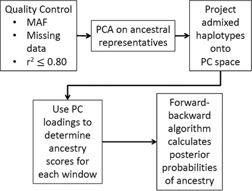
Our approach is outlined in Figure 1. Briefly, the method uses PCA to determine how informative each SNP is in classifying the ancestry of a genetic region. These PC loadings are used as weights in a weighted average of the allele values in a window of SNPs, and the resulting window scores are used as the observed values in a HMM to assign posterior probabilities to the ancestry in each window. While the details of this approach are discussed below, the website for the algorithm can be accessed at https://sites.google.com/site/pcadmix/home.

Figure 1.

Outline of the PCAdmix algorithm.

PCAdmix Algorithm: Quality Control and PCA

An initial quality-control filter removed SNPs with high missingness and low minor-allele frequency. A liberal LD filter was then applied, removing one of each pair of SNPs with r² > 0.80 in any of the ancestral or admixed groups. This prevents high-LD blocks from having excessive influence on the inferred ancestry of a region, while retaining a dense, informative set of SNPs. We used Singular Value Decomposition in R (R Development Core Team 2010) to infer PCs of the phased genotypes of the ancestral representatives. We then projected phased genotypes of admixed individuals onto the basis of PCs. The observed ancestry score for haplotype i in window w is the weighted sum S_iw = L_wg_iw, where g_iw is a column vector of the haplotype’s alleles in the window, standardized by the mean and standard deviation in the ancestral populations, and L_w is a matrix such that each column contains the PC loadings of one SNP in the window. The vector S_iw contains the ancestry scores across the first K-1 PCs, where K is the number of ancestral populations.

PCAdmix Algorithm: Forward-Backward Algorithm

The posterior probabilities of each ancestry for each window were then computed by a forward-backward algorithm, a method of computing posterior probabilities for states in an HMM. The transition probabilities for the HMM followed a haploid version of those in the Viterbi algorithm ofBryc et al. (2010), which is based on the population genetic model ofFalush et al. (2003) and of Li and Stephens (2003). The transition probability is defined by π, the probability of recombination between windows, and q_i,j, the frequency of the target population’s chromosomes in the admixing ancestral pool:

$$P(an{c}_{i,w}=j|an{c}_{i,w-1}=k)=\{\begin{array}{cc}{q}_{i,j}\mathbf{\pi }\hfill & \text{if}k\ne j\hfill \\ q_{i,j}\mathbf{\pi }+(1-\mathbf{\pi })\hfill & \text{if}k=j\hfill \end{array}$$ (1)

where anc_i,w is the ancestry of haplotype i at window w, q_i,j is the chromosome-wide proportion of population j ancestry in this haploid chromosome, and π = 1 − exp(dĜ) is the probability of a single recombination having occurred in the distance d (in Morgans) between the midpoints of windows w−1 and w, during the estimatedĜ generations since admixture. We assume that the windows are sufficiently dense so that the probability of two or more recombination events between adjacent windows is negligible, an assumption that should be reasonable for admixture that is recent relative to the window size. As demonstrated below, our method is robust to misestimation of G, which suggests that it is also robust to multiple recombinations.

For a given haplotype i, q_i,j represents the frequency of population j’s chromosomes in the admixing ancestral pool for haplotype i. In other words, q_i,j represents the average ancestry proportion of population j in haplotype i. The value q_i,j is estimated by

$$q_{i,j}=\frac{D_{i,j}}{\sum _k{D}_{i,k}^{\prime }}$$ (2)

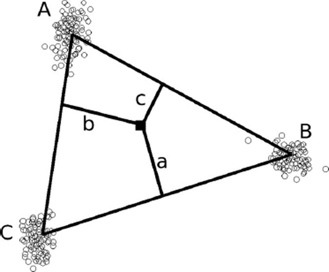
where D_i,j is the Euclidean distance in PC-space from haplotype i to the hyperplane containing the mean window scores of all ancestral populations other than j, as shown in Figure 2. Therefore, a haplotype that falls far from the mean of population j will have small values for D_i,j and q_i,j. To ensure nonzero transition probabilities, we restricted 0.01 ≤ q_i,j ≤ 0.99 for all j.

Figure 2.

Estimation of average ancestry proportion for a haplotype. For k = 3 ancestral populations, the population A average ancestry proportion of each haplotype (black square) is estimated by that haplotype’s distance from the line connecting the means of the other two populations on the first and second principal components, as a proportion of the haplotype’s total distance from all edges: q_i,A = a/(a + b + c).

The emitted window scores are modeled by a multivariate normal distribution: S_iw | (anc_i,w = j) ~ N(µ_jw, Σ_jw), where S_iw is the vector of ancestry scores for admixed haplotype i in window w, Σ_jw is a vector containing ancestral population j’s mean scores for this window on the first K-1 PCs, and Σ_jw is the covariance matrix of the scores for this window among the population j haplotypes. To ensure nonzero emission probabilities, we require that each entry of Σ_jw equals the maximum of the empirical covariance and 0.0001, and that cov(S_iw,a, S_iw,b) < var(S_iw,a), var(S_iw,b), where a and b are distinct PCs.

By using the transition and emission probabilities described above, a forward-backward algorithm is applied to find the posterior probability that each window in each admixed haplotype originates from population 1, 2,… K. The posterior probabilities may be used directly, or used to make hard assignments of ancestry if the posterior probability exceeds a threshold.

Analysis of Simulated Admixture

We tested our method on simulated admixed individuals with ancestry from both two and three populations. Haploid genomes from the ancestral populations were chosen as ancestors, and recombination breakpoints (potential ancestry change-points) were chosen by simulating a Poisson process. Simulated chromosomes were then assembled by combining genomic segments from the ancestors at each recombination breakpoint. The true ancestors used to generate the admixed individuals were removed from the pool of ancestral representatives before analysis. Accuracy was defined as the proportion of SNPs assigned to the correct simulated ancestry. To assess accuracy, we used all the SNPs from the original data set, while the windows were defined by the SNPs that passed the LD and MAF filters for inclusion in the PCA. SNPs that fell before the first window on the chromosome or after the last window, and SNPs that fell between windows assigned to different ancestries, were excluded from the accuracy calculation, as no ancestry can be assigned to these SNPs.

Simulations with Two Ancestral Populations

For the two-population simulations, ancestral haplotypes were chosen from the International HapMap3 project (Altshuler et al. 2010) (http://hapmap.ncbi.nlm.nih.gov/), with one ancestor chosen from Utah individuals of European descent (CEU) and the other from Yoruba individuals from Nigeria (YRI), simulating the largely West African ancestry of African American individuals (Salas et al. 2005). The distribution of recombination breakpoints was generated by using eight generations since admixture (G = 8), and genomic segments were chosen from ancestors according to freq(YRI) Beta (12,3) to model the average African ancestry proportion among African Americans, approximately 80% (Bryc et al. 2010). Variants with r² > 0.80 were removed, and 12 simulated haplotypes were analyzed with PCAdmix and HAPMIX by using Ĝ = 8, the true parameter value. PCAdmix was run with a window size of 20 SNPs. We also tested our method’s robustness to the choice of parameter values by allowing Ĝ to vary from 1 to 128, the number of SNPs per window to vary from 1 to 160, and the LD filtering to vary from an r² threshold of 0.80 to no LD filtering. Finally, we examined our method’s robustness to the choice of ancestral representatives by analyzing the simulated haplotypes with the true populations (YRI and CEU), sets of three populations [YRI, CEU, and Han Chinese and Japanese (CHB-JPT) or Italian (TSI)], and misspecified ancestral populations by using Luhya (LWK) or Maasai (MKK) to represent YRI ancestry. These populations are likely to be poor ancestral proxies because they are East African populations, whereas the simulated haplotypes were sampled from individuals from a West African population, the Yoruba. The F_ST between Luhya and Yoruba is 0.0080 and between Maasai and Yoruba is 0.027 (Altshuler et al. 2010).

Simulations with Three Ancestral Populations

For the three-population simulations, ancestors were chosen from the HGDP (Cann et al. 2002) data (http://hagsc.org/hgdp/files.html). Genomic segments from Yoruba and French chromosomes were combined with segments from each of 29 other populations. The locations of recombination breakpoints were simulated by using a Poisson distribution with a parameter determined by the genetic distance as determined from HapMap data. Genomic segments were chosen from the ancestors with equal probability at each recombination breakpoint. The data were analyzed with the use of the same parameters as described for the two-population simulations. For comparison with LAMP (Pasaniuc et al. 2009), the four simulated chromosomes from each set of ancestries were combined into diploid individuals. LAMP v. 2.5 was run by using Ĝ = 8, recombination rate = 10⁻⁸, offset = 0.2, and LD independence threshold = 0.1. The mixture proportion α for each population was set to the average of the ancestry proportions estimated by PCAdmix. LAMP was run by using its forward-backward algorithm for comparison with PCAdmix. Two sets of simulations were also run by using LAMP’s default maximum likelihood method; accuracies were found to be similar between the two methods. A SNP was called as having homozygous ancestry if the locus-specific ancestry from one population was 0.8, and having heterozygous ancestry if the locus-specific ancestries from two populations were 0.4. For comparison with LAMP, the diploid accuracy of PCAdmix was also computed on regions where PCAdmix assigned ancestry to both haplotypes, by using a calling threshold of 0.8.

To investigate how to optimize accuracy when populations are closely related, we further analyzed the Yoruba-French-Basque simulations by using a variety of parameters; the F_ST on chromosome 1 between the HGDP French and Basque samples is 0.0031. We testedĜ = 1, 4, 8, 12, 16; MAF ≥0.10, 0.05, and 0; window sizes from 10 to 90 SNPs, and r² ≤0.80, 0.90, and 1.0. Because the challenge in assigning ancestry for admixtures of closely related populations stems from the fact that the ancestral populations are genetically similar and overlap in the space of PCs, we also tested four systems for filtering the ancestral haplotypes to enhance their distinctness: In method A, we performed PCA on the Yoruba, French, and Basque samples, and we removed the two French haplotypes that fell closest to the Basque mean on the second PC (PC2), and vice versa for two Basque haplotypes. In method B, we removed French haplotypes that fell closer to the Basque mean on PC2 than the most French-looking Basque haplotype, and vice versa for removing Basque haplotypes. In method C, we performed PCA on the French and Basque samples only, and then we excluded ancestral haplotypes that were more extreme than the admixed haplotype that fell closest to that population’s mean on PC1 (Figure S1 in the Appendix). This method could result in an unnecessary reduction in sample size if the admixed individuals spanned a wide range of ancestry proportions. Therefore, we also explored method D, which excluded a different set of ancestral haplotypes for each admixed haplotype. For each admixed haplotype, we excluded the French haplotypes that fell closer to the Basque mean on PC1 than that admixed haplotype, and similarly for Basque haplotypes. Finally, we tested the application of a “disambiguation” phase, performing a two-population analysis of the regions that were initially assigned as French or Basque.

Application

We used our method to examine three-way European, Native American, and African admixture in Latino individuals from the NYULatino project (Bryc et al. 2010). These individuals had origins in Ecuador, Colombia, Puerto Rico, and the Dominican Republic. European and African ancestral populations were represented by CEU and YRI individuals from HapMap3, and the Native American ancestral population was represented by Maya, Pima, Karitiana, Surui, and Colombian individuals from HGDP (Rosenberg et al. 2002) that were estimated to have less than 5% genome-wide European ancestry using FRAPPE (Tang et al. 2005). We filtered SNPs using MAF > 10%, missingness <10% in the combined dataset of the ancestral representatives, and pairwise r² ≤0.80 in the full HapMap3 data set. After filtering, 380,360 autosomal SNPs remained. We ran PCAdmix by using a window size of 20 SNPs and Ĝ = 8. Native American haplotypes were phased with use of IMPUTE v.2.1.0 (Howie et al. 2009) by using 110 iterations, 10 iterations of burn-in, and 120 conditioning states, the same protocols as used for phasing by the HapMap 3 project (http://hapmap.ncbi.nlm.nih.gov/downloads/phasing/2009-02_phaseIII/HapMap3_r2/hapmap3_r2_phasing_summary.doc).

After assigning ancestry along each chromosome, we computed the African, European, and Native American ancestry proportions in each window of each of the four Latino populations. Regions with ancestry proportions falling more than three SDs from each Latino population’s genome-wide mean were considered to have “extreme” ancestry. To illustrate the utility of a haplotype-based approach to ancestry assignment, we also tested for assortative mating (Risch et al. 2009) by examining the correlation between ancestry probabilities for pairs of phased haplotypes and the proportion of windows at which haplotype pairs shared the same ancestry. To test the significance of these values, we permuted the haplotype labels 1,000 times within each Latino population sample.

Results

Simulations with Two Ancestral Populations

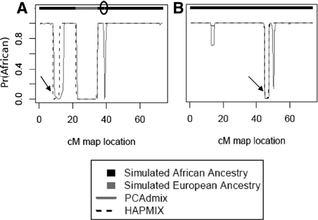
Both PCAdmix and HAPMIX were highly accurate in assigning ancestry along simulated chromosomes, with increasing accuracy at more stringent calling thresholds (Table S1 in the Appendix). HAPMIX performed slightly better than our method because of a lower number of short regions of spurious inferred European ancestry. However, HAPMIX was also less sensitive to short regions of true ancestry (Figure 3a). It is interesting to note that HAPMIX and PCAdmix agreed in the two longest tracts of incorrect ancestry assignment made by either method (Figure 3a and b), suggesting that the Yoruba individuals used to simulate these segments may in fact have some European ancestry or that some CEU individuals used as ancestral representatives in the analysis may have African ancestry, leading to poor disambiguation between these populations.

Figure 3.

Comparison of PCAdmix and HAPMIX on simulated chromosomes. (A) and (B) are two examples of simulated chromosomes. Top bar indicates the simulated ancestry of each chromosome (black = YRI, gray = CEU). Solid and dashed lines indicate the posterior probability of YRI ancestry at that window, using our method (solid) and HAPMIX (dashed). The black oval indicates a short region of European ancestry. The black arrows indicate regions where both methods inferred European ancestry, although the segment was simulated from a YRI haplotype.

Our method is robust to the choice of the number of SNPs per window (Table S2 in the Appendix). This demonstrates that the method picks up consistent signals in the data, not artifacts of window subdivisions. As expected, using fewer than 10 SNPs per window (resulting in an average window length of <22.3 kb) increases the number of spurious short ancestry regions identified, decreasing accuracy.

Our method, like HAPMIX, is robust to the estimate of G, the number of generations since admixture (Table S3 in the Appendix). This robustness is an advantage to researchers interested in mapping ancestry tracts, but it may prove a challenge for fine-scale estimation of the timing of admixture events. Accuracy was slightly higher when G was somewhat underestimated than whenĜ = G, because of the improved smoothing over noisy window scores.

When the Luhya or Maasai were used as ancestral representatives for the Yoruba, our method’s accuracy was essentially unchanged (Table 1), although these ancestral groups are genetically distinct, with F_ST = 0.0080 between Luhya and Yoruba and F_ST = 0.027 between Maasai and Yoruba. Using a simple Wright-Fisher model (Durrett 2008) to generate forward simulations shows that 97.9% of the time, the F_ST between a population with effective population size = 5,000, and the same population after 100 generations of drift is <0.027. This suggests that modern-day sampled individuals can be used as representatives for ancestral populations from previous generations without loss of accuracy because of genetic drift.

Table 1.

Accuracy under Different Assumptions about the Ancestral Populations; the True Ancestry Was YRI-CEU

Tested Ancestry	Overall Accuracy (%)	Accuracy YRI	Accuracy CEU
YRI-CEU	98.1	97.7	99.3
MKK-CEU	98.2	98.3	97.9
LWK-CEU	97.9	97.5	99.1
YRI-CEU-(CHB-JPT)	97.2	96.8	98.7
YRI-CEU-TSI	86.1	97.5	51.6

Accuracy percentage listed is for a calling threshold of 0.5 (for two ancestral populations) or 1/3 (for three ancestral populations). Accuracy YRI indicates accuracy for regions where the true ancestry was YRI.

Our method retained excellent accuracy (97.2%) when HapMap3 Han Chinese and Japanese (CHB-JPT) individuals were used as a third, spurious ancestral population, with only two simulated African American haplotypes showing small regions assigned to CHB-JPT ancestry. In contrast, when the spurious ancestral population is closely related to one of the true ancestral populations, as in the YRI-CEU-TSI analysis, which has F_ST (CEU-TSI) = 0.0040 (Altshuler et al. 2010), our method experienced a 12.0 percentage-point reduction in accuracy (down to 86.1%) because of loss of disambiguation between CEU and TSI populations. The accuracy for SNPs whose true background is YRI remains high (97.5% at a calling threshold of 1/3, that is, assigning all SNPs) (Table 1), but the accuracy for SNPs whose true background is CEU is no better than random guessing (51.6% for calling threshold =1/3) and is not improved by the use of a more stringent calling threshold.

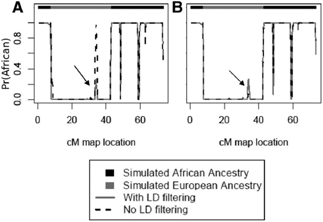
As shown in Figure 4a, LD filtering decreases the intensity of some, but not all, spurious deviations from the true ancestry. A similar effect can be obtained without LD filtering by increasing the number of SNPs per window (Figure 4b), increasing the amount of information about the window’s true ancestry to contrast with spurious ancestral information provided by a small cluster of high-LD SNPs.

Figure 4.

Effects of LD filtering on a simulated chromosome. (A) 20 SNPs per window. Solid line = data filtered to r² ≤ 0.80; dashed line = data without filtering. (B) Solid line = 20 SNPs per window, with LD filtering; dashed line = 40 SNPs per window without filtering. Black arrows indicate a region of European ancestry which is correctly assigned when LD filtering is used or when the window size is 40 SNPs.

Simulations with Three Ancestral Populations

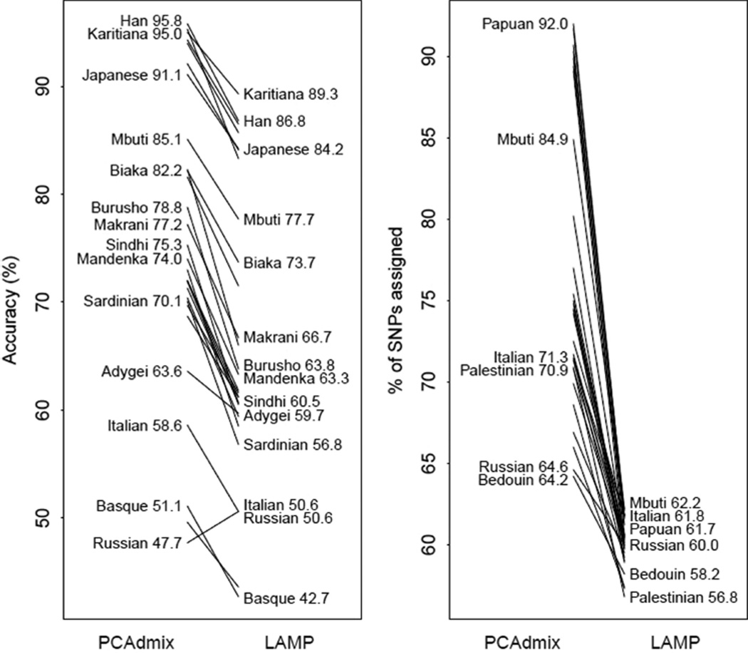
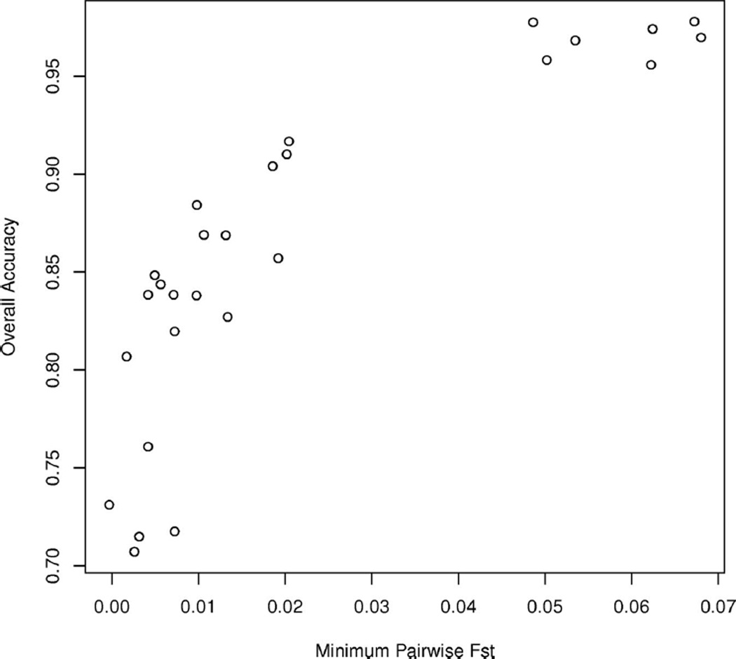
In the three-population simulations, PCAdmix had high accuracy on a per-chromosome and per-diploid individual basis (Figure 5, Table S4 in the Appendix). PCAdmix had higher accuracy than LAMP across 28 of the 29 simulations. PCAdmix was also able to assign ancestry to a greater proportion of SNPs. This reflects the fact that the LD filtering for PCAdmix is much less stringent than that for LAMP, permitting ancestry assignment at a denser set of SNPs. It also indicates that PCAdmix’s superior accuracy was not because of the choice of calling thresholds. As expected, accuracy was higher when the three ancestral populations were more differentiated (Figure 6).

Figure 5.

Diploid accuracy and call rate of PCAdmix and LAMP. Assigned % is out of 43,518 SNPs. Chromosomes were simulated with ancestry from three populations, including Yoruba and French. Labeled populations are the third population included in simulations. Biaka = Biaka Pygmies; Mbuti = Mbuti Pygmies; Italian = North Italian.

Figure 6.

Accuracy vs. minimum F_ST. Shown is the overall accuracy on three-population simulations vs. the minimum pairwise F_ST among the three populations.

For the Yoruba-French-Basque analysis, the baseline haploid accuracy was 71.5% with r² ≤ 0.80, Ĝ = 8, and 20 SNPs per window. Underestimating the number of generations since admixture, while effective in decreasing the rate of spurious ancestry transitions in the two-population simulations, did not improve the accuracy in the Yoruba-French-Basque analysis. This is likely because of the fact that a majority of the errors in classifying French and Basque tracts spanned multiple windows, so reducing the transition rate of the HMM did not substantially change results. In contrast, increasing Ĝ to 12 improved the accuracy to 72.4%. Windows longer than 20 SNPs, particularly in conjunction with more liberal MAF or LD thresholds for SNP inclusion, also improved accuracy. For this simulation scenario, the best analysis combination was 50 SNPs per window with MAF ≥ 0, which gave an accuracy of 73.9%.

Removing the ancestral haplotypes that closely resembled typical haplotypes of the other population was also effective; the most effective method was method C. This method increased overall accuracy from 71.5% to 73.6%. A disambiguation phase slightly improved overall accuracy from 71.5% to 72.0%. We also tested all possible combinations of the four best-performing methods (Ĝ = 12, 50 SNPs per window with MAF ≥ 0, filtering by method C, and implementing a disambiguation phase). The best overall accuracy, 74.8%, resulted from the combination of all these methods except Ĝ = 12.

An identical strategy was also effective in slightly increasing the accuracy on other combinations of closely related populations: Applying this combination of three methods to Yoruba-French-Russian (French-Russian F_ST = 0.0026 for chromosome 1 of HGDP data) increases the accuracy from 70.7% to 71.8%. Applying it to Han Chinese-Japanese-Yoruba (Han Chinese-Japanese F_ST = 0.0035) increased the accuracy from 83.4% to 84.4%. Applying it to Yoruba-French-North Italian (French-North Italian F_ST = 0.00034 for chromosome 1 of HGDP data) increases the accuracy from 73.1% to 73.7%. It is likely that the accuracy on these simulations could be increased somewhat further by fine-tuning the parameter values to suit the particular combinations of populations. In a situation with real data, this could be done by selecting parameter values that optimize accuracy on simulated haplotypes that resemble the true admixed individuals.

Application

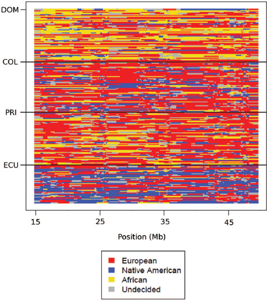
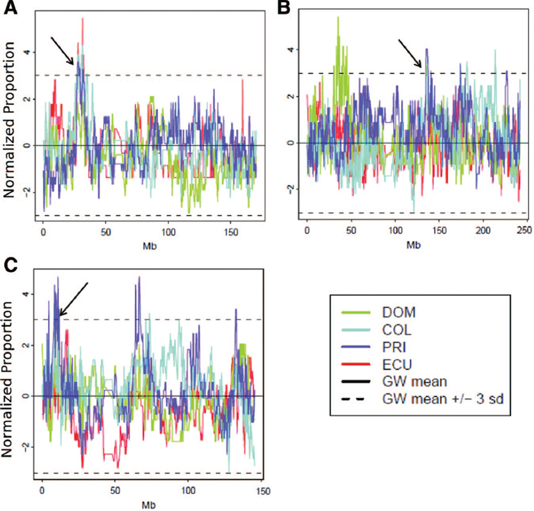
In the analysis of the NYULatino data, Dominicans showed the largest mean proportion of African ancestry (39.5%), followed by Puerto Ricans (21.1%). Ecuadorians had the largest mean proportion of Native American ancestry (47.4%), followed by Colombians (30.0%). These results agree with expectations based on historical information and previous results with use of FRAPPE (Bryc et al. 2010). While most ancestry tracts spanned many windows (73% of the tracts were >1 Mb in length), some parts of the genome exhibited rapid switching of ancestry (Figure 7). All four Latino populations showed evidence of assortative mating (P < 0.001 for correlation of ancestry probability and for shared ancestry). This confirms and extends the results ofRisch et al. (2009), who found assortative mating in Puerto Ricans on the basis of 104 ancestry-informative markers. We identified 12 regions having extreme levels of shared ancestry in more than one population (Table 2). In particular, a pair of regions on chromosome 6 showed elevated levels of African ancestry in three of the four Latino populations, and regions on chromosomes 2 and 8 showed elevated levels of Native American ancestry in three of the four Latino populations (Figure 8).

Figure 7.

Analysis of Latino individuals using PCAdmix. Chromosome 22 is shown. We used a calling threshold of 0.9. DOM = Dominican; COL = Colombian; PRI = Puerto Rican; ECU = Ecuadorian.

Table 2.

Regions with Extreme Ancestry Proportions in Multiple Latino Populations.

Chromosome	Position (Mb)	Ancestry	Populations
2	136.8–136.9	NAmer	COL, DOM, PRI
6	27.3–28.8	YRI	COL, ECU, PRI
6	31.4–31.5	YRI	COL, ECU, PRI
8	10.8–10.9	NAmer	COL, DOM, PRI
2	134.9–135.5	NAmer	DOM, PRI
5	30.5–30.9	YRI	COL, ECU
8	8.4–8.8	NAmer	DOM, PRI
11	87.5–87.6	YRI	COL, PRI
13	58.3–58.5	NAmer	DOM, PRI
15	59.7–59.8	YRI	ECU, PRI
15	60.8–61.0	YRI	ECU, PRI
15	66.8–67.5	YRI	COL, ECU

All regions shown here exhibited ancestry proportions more than three standard deviations above the genome-wide mean for that ancestral population. YRI = Yoruba (African); Namer = Native American; COL = Colombian; DOM = Dominican; ECU = Ecuadorian; PRI = Puerto Rican.

Figure 8.

Normalized ancestry proportions in Latino populations. Dashed lines indicate values that are three SDs from the mean. Black arrows indicate regions where three Latino populations share high proportions of African or Native American ancestry. (A) African ancestry proportion on chromosome 6. (B) Native American ancestry on chromosome 2. (C) Native American ancestry on chromosome 8. GW = Genome-wide; SD = standard deviation.

We examined 19,018 windows across the genome in four populations. Therefore, for a single population’s ancestry proportion to be significantly above the genome-wide mean at the α = 0.05 level would require a P value (assuming Bonferroni correction for multiple testing) of 6.57e-07, equivalent to an ancestry proportion of 4.84 SDs from the genome-wide mean. Three regions reached this level of significance (Table S5 in the Appendix). None of these regions were significant in more than one admixed population examined.

Discussion

In this paper, we have presented a PC-based approach to assigning ancestry along the genome in admixed individuals. Our approach has similar accuracy to HAPMIX for two-way population admixture, and better accuracy and calling rate than LAMP for three-way population admixture. This superior accuracy may be due in part to the fact that our method utilizes haplotypes from ancestral representatives, whereas LAMP uses ancestral allele frequencies that do not provide information about LD in the ancestral populations. Our approach is robust to the choice of window size, to misspecification of ancestral populations, and to the estimated time since admixture. We have implemented our method in the software PCAdmix, which is freely available for academic use as a compiled binary at https://sites.google.com/site/pcadmix/.

In the NYULatino data, rapid ancestry switching is present in some parts of the genome. Further investigation of these short segments is warranted; those that persist across many values of Ĝ and many calling thresholds may indicate recombination hotspots. In contrast, ancestry segments with only intermediate posterior probability that disappear under analysis with lower values of Ĝ (and therefore, lower transition probabilities) may be artifacts of the analysis, because of the fact that the ancestry with maximum marginal posterior probability for a given window is not necessarily concordant with the most likely ancestry “path” through the chromosome.

We identified 12 regions having extreme levels of shared ancestry in more than one Latino population. Some of these regions are close together, indicating that they may reflect a smaller number of larger regions of elevated ancestry levels. These regions may have reached their extreme levels of ancestry because of selection during or after the initiation of admixture. In particular, the region on chromosome 2 is near the LCT locus (136.5–136.6 Mb) for lactase persistence (Harvey et al. 1993), a known target of selection (Tishkoff et al. 2007). The regions on chromosome 6 are close to the human leukocyte antigen loci (around 30–32 Mb), which play an important role in immunity.Tang et al. (2007) also found a region on chromosome 6 centered at 28.8 Mb to have elevated African ancestry in Puerto Ricans. It would be intriguing to find evidence of selection in this important region, whether the selection is in the form of large genetic differentiation between the true and proxy ancestral populations, leading to biases in local ancestry estimates, or in the form of balancing selection in the admixed population, favoring more-diverse African haplotypes. However, this peak could also be explained as an artifact of the unusual long-range LD that occurs in this region (Price et al. 2008). Furthermore, none of these regions achieved statistical significance in more than one population, so we cannot reject the null hypothesis of no selection. It would be valuable to pursue further investigation of haplotype diversity on chromosome 6 and the other regions in Table 2 to understand the sources of the elevated ancestry sharing in each region.

A potential limitation of our method is that it uses phased genotype data, requiring family- or population-based phasing prior to ancestry deconvolution. Analysis of phased data is advantageous because it provides information about the distinct ancestry of an individual’s parents and permits haplotype-based analyses of the population genetic history of admixture events, such as assortative mating. However, worth noting is that errors in phasing can result in errors in ancestry assignment. In particular, phasing errors may complicate population genetic inference for regions of the genome where an individual has ancestry from two different populations. However, our findings of assortative mating in Latinos depend on regions where individuals have diploid ancestry from a single population, so they are much more likely to remain valid in the presence of possible phasing errors. Phasing errors are becoming less common as phasing methods improve and efforts such as the 1,000 Genomes Project (Durbin et al. 2010) produce larger pools of genotypes that can be used as references during phasing; however, it would be valuable to extend PCAdmix to unphased data, as well as to investigate the effectiveness of iterative phasing and ancestry assignment, employing reference panels conditional on estimated local ancestry.

We found that filtering ambiguous ancestral haplotypes, along with modifying parameters of analysis and implementing a disambiguation phase, produced modest improvements in accuracy. When filtering-method C was applied to the Yoruba-French-Basque simulations, overall accuracy increased from 71.5% to 73.6%. While this increase is small, it is valuable to note that accuracy can be somewhat improved simply through the choice of more informative ancestral representatives. In the future, it would be worthwhile to explore additional methods of filtering ancestral representatives for optimal accuracy. In addition, small increases in overall accuracy can reflect larger improvements in the accuracy of classifying genomic regions from a particular population; in these simulations, using method C increased the accuracy of classifying true Basque regions from 56.2% to 61.4%. Such population-specific improvements would be of particular interest when the genomes of admixed individuals are used to understand the genome of a specific ancestral population, such as ancestral populations with few extant unadmixed individuals (Byrnes et al. 2011).

When distinguishing ancestry from closely related populations, filtering ancestral representatives according to Model C could result in an imbalance of ancestral representative sample sizes if the ancestry proportions from the two closely related populations were very different (e.g., 60% French and 5% Basque, in addition to 35% Yoruba). This could result in a distortion of the PCA projection (McVean 2009), which could reduce the accuracy of the estimated ancestry proportions. This was not a problem in our simulations, where Model C excluded just 2 Basque haplotypes and 7 French haplotypes (out of 44 haplotypes from each population). However, additional approaches to filtering the ancestral representatives should be investigated for admixed individuals with less balanced ancestry proportions. One possibility would be to exclude equal numbers of haplotypes from each population, as in model A, but to determine the number of excluded haplotypes by the location of admixed individuals in PC-space, as in models C or D.

PCAdmix utilizes haplotypes from ancestral representatives to assign ancestry to admixed haplotypes. In our simulations, we found that the accuracy of PCAdmix was robust to mis-specification of ancestral populations, suggesting that modern individuals can be used to represent historical ancestral populations. However, some ancestral populations may not have unadmixed modern representatives. In the future, it would be valuable to enhance PCAdmix by an investigation of iterative ancestry approximation when ancestral representatives are not available; as discussed by McVean (2009), admixture proportions are detectable even without source populations for up to 15 generations after admixture. Further extensions could allow the number of SNPs per window to vary throughout the genome to better distribute information across windows and to allow different estimates of G for different pairs of populations.

We have demonstrated that our method is useful in identifying regions of extreme ancestry proportions within populations, which may indicate sites of selection during or after the process of admixture. Our method is a computationally fast algorithm that allows for multi-population ancestry estimation, which will have applications for large data sets of multi-way admixed populations, such as Latinos, North and East Africans (who have admixture from Chadic, West African and Middle Eastern populations) (Jakobsson et al. 2008), South African Cape Coloured (de Wit et al. 2010), and other worldwide populations. Our method will be valuable for improving the understanding of the population genetic history of admixed populations and for admixture mapping on dense genome-wide data.

Literature Cited

- Alexander DH, Novembre J, Lange K. Fast model-based estimation of ancestry in unrelated individuals. Genome Res. 2009;19:1655–1664. doi: 10.1101/gr.094052.109. [DOI] [PMC free article] [PubMed] [Google Scholar]
- Altshuler DM, Gibbs RA, Peltonen L, et al. Integrating common and rare genetic variation in diverse human populations. Nature. 2010;467:52–58. doi: 10.1038/nature09298. [DOI] [PMC free article] [PubMed] [Google Scholar]
- Bryc K, Auton A, Nelson MR, et al. Genome-wide patterns of population structure and admixture in West Africans and African Americans. Proc. Natl. Acad. Sci. USA. 2010a;107:786–791. doi: 10.1073/pnas.0909559107. [DOI] [PMC free article] [PubMed] [Google Scholar]
- Bryc K, Velez C, Karafet T, et al. Colloquium paper: Genome-wide patterns of population structure and admixture among Hispanic/Latino populations. Proc. Natl. Acad. Sci. USA. 2010b;1072(Suppl.):8954–8961. doi: 10.1073/pnas.0914618107. [DOI] [PMC free article] [PubMed] [Google Scholar]
- Byrnes JK, Rodríguez-Flores JL, Moreno-Estrada A, et al. Genomic Reconstruction of an Extinct Population from Next-Generation Sequence Data—Insights from the Taìno Genome Project; Platform presentatiom at International Congress of Human Genetics; 13 October 2011; Montreal, Canada. 2011. [Google Scholar]
- Cann HM, de Toma C, Cazes L, et al. A human genome diversity cell line panel. Science. 2002;296:261–262. doi: 10.1126/science.296.5566.261b. [DOI] [PubMed] [Google Scholar]
- Chapman NH, Thompson EA. The effect of population history on the lengths of ancestral chromosome segments. Genetics. 2002;162:449–458. doi: 10.1093/genetics/162.1.449. [DOI] [PMC free article] [PubMed] [Google Scholar]
- de Wit E, Delport W, Rugamika CE, et al. Genome-wide analysis of the structure of the South African coloured population in the Western Cape. Hum. Genet. 2010;128:145–153. doi: 10.1007/s00439-010-0836-1. [DOI] [PubMed] [Google Scholar]
- Durbin RM, Abecasis GR, Altshuler DL, et al. A map of human genome variation from population-scale sequencing. Nature. 2010;467:1061–1073. doi: 10.1038/nature09534. [DOI] [PMC free article] [PubMed] [Google Scholar]
- Durrett R. Probability Models for DNA Sequence Evolution. New York: Springer Verlag; 2008. [Google Scholar]
- Engelhardt BE, Stephens M. Analysis of population structure: A unifying framework and novel methods based on sparse factor analysis. PLoS Genet. 2010;6:e1001117. doi: 10.1371/journal.pgen.1001117. [DOI] [PMC free article] [PubMed] [Google Scholar]
- Falush D, Stephens M, Pritchard JK. Inference of population structure using multilocus genotype data: Linked loci and correlated allele frequencies. Genetics. 2003;164:1567–1587. doi: 10.1093/genetics/164.4.1567. [DOI] [PMC free article] [PubMed] [Google Scholar]
- Gompert Z, Parchman TL, Buerkle CA. Genomics of isolation in hybrids. Phil. Trans. R. Soc. B. 2012;367:439–450. doi: 10.1098/rstb.2011.0196. [DOI] [PMC free article] [PubMed] [Google Scholar]
- Harvey CB, Fox MF, Jeggo PA, et al. Regional localization of the lactase-phlorizin hydrolase gene, LCT, to chromosome 2q21. Ann. Hum. Genet. 1993;57:179–185. doi: 10.1111/j.1469-1809.1993.tb01593.x. [DOI] [PubMed] [Google Scholar]
- Howie BN, Donnelly P, Marchini J. A flexible and accurate genotype imputation method for the next generation of genome-wide association studies. PLoS Genet. 2009;5:e1000529. doi: 10.1371/journal.pgen.1000529. [DOI] [PMC free article] [PubMed] [Google Scholar]
- Jakobsson M, Scholz SW, Scheet P, et al. Genotype, haplotype and copy-number variation in worldwide human populations. Nature. 2008;451:998–1003. doi: 10.1038/nature06742. [DOI] [PubMed] [Google Scholar]
- Jin W, Xu S, Wang H, et al. Genome-wide detection of natural selection in African Americans pre-and post-admixture. Genome Res. 2011;22:519–527. doi: 10.1101/gr.124784.111. [DOI] [PMC free article] [PubMed] [Google Scholar]
- Li N, Stephens M. Modeling linkage disequilibrium and identifying recombination hotspots using single-nucleotide polymorphism data. Genetics. 2003;165:2213–2233. doi: 10.1093/genetics/165.4.2213. [DOI] [PMC free article] [PubMed] [Google Scholar]
- McVean G. A genealogical interpretation of principal components analysis. PLoS Genet. 2009;5:e1000686. doi: 10.1371/journal.pgen.1000686. [DOI] [PMC free article] [PubMed] [Google Scholar]
- Pasaniuc B, Sankararaman S, Kimmel G, et al. Inference of locus-specific ancestry in closely related populations. Bioinformatics. 2009;25:i213–221. doi: 10.1093/bioinformatics/btp197. [DOI] [PMC free article] [PubMed] [Google Scholar]
- Pasaniuc B, Zaitlen N, Lettre G, et al. Enhanced statistical tests for GWAS in admixed populations: Assessment using African Americans from CARe and a Breast Cancer Consortium. PLoS Genet. 2011;7:e1001371. doi: 10.1371/journal.pgen.1001371. [DOI] [PMC free article] [PubMed] [Google Scholar]
- Patterson N, Price AL, Reich D. Population structure and eigenanalysis. PLoS Genet. 2006;2:e190. doi: 10.1371/journal.pgen.0020190. [DOI] [PMC free article] [PubMed] [Google Scholar]
- Pool JE, Nielsen R. Inference of historical changes in migration rate from the lengths of migrant tracts. Genetics. 2009;181:711–719. doi: 10.1534/genetics.108.098095. [DOI] [PMC free article] [PubMed] [Google Scholar]
- Price AL, Tandon A, Patterson N, et al. Sensitive detection of chromosomal segments of distinct ancestry in admixed populations. PLoS Genet. 2009;5:e1000519. doi: 10.1371/journal.pgen.1000519. [DOI] [PMC free article] [PubMed] [Google Scholar]
- Price AL, Weale ME, Patterson N, et al. Long-range LD can confound genome scans in admixed populations. Am. J. Hum. Genet. 2008;83:132–135. doi: 10.1016/j.ajhg.2008.06.005. [DOI] [PMC free article] [PubMed] [Google Scholar]
- Pugach I, Matveyev R, Wollstein A, et al. Dating the age of admixture via wavelet transform analysis of genome-wide data. Genome Biol. 2011;12:R19. doi: 10.1186/gb-2011-12-2-r19. [DOI] [PMC free article] [PubMed] [Google Scholar]
- R Development Core Team. R: A Language and Environment for Statistical Computing. Vienna, Austria: 2010. [Google Scholar]
- Risch N, Choudhry S, Via M, et al. Ancestry-related assortative mating in Latino populations. Genome Biol. 2009;10:R132. doi: 10.1186/gb-2009-10-11-r132. [DOI] [PMC free article] [PubMed] [Google Scholar]
- Rosenberg NA, Pritchard JK, Weber JL, et al. Genetic structure of human populations. Science. 2002;298:2381–2385. doi: 10.1126/science.1078311. [DOI] [PubMed] [Google Scholar]
- Salas A, Carracedo A, Richards M, et al. Charting the ancestry of African Americans. Am. J. Hum. Genet. 2005;77:676–680. doi: 10.1086/491675. [DOI] [PMC free article] [PubMed] [Google Scholar]
- Stam P. The distribution of the fraction of the genome identical by descent in finite random mating populations. Genet. Res. 1980;35:131–155. [Google Scholar]
- Tang H, Choudhry S, Mei R, et al. Recent genetic selection in the ancestral admixture of Puerto Ricans. Am. J. Hum. Genet. 2007;81:626–633. doi: 10.1086/520769. [DOI] [PMC free article] [PubMed] [Google Scholar]
- Tang H, Coram M, Wang P, et al. Reconstructing genetic ancestry blocks in admixed individuals. Am. J. Hum. Genet. 2006;79:1–12. doi: 10.1086/504302. [DOI] [PMC free article] [PubMed] [Google Scholar]
- Tang H, Peng J, Wang P, et al. Estimation of individual admixture: analytical and study design considerations. Genet. Epidemiol. 2005;28:289–301. doi: 10.1002/gepi.20064. [DOI] [PubMed] [Google Scholar]
- Tishkoff SA, Reed FA, Ranciaro A, et al. Convergent adaptation of human lactase persistence in Africa and Europe. Nat. Genet. 2007;39:31–40. doi: 10.1038/ng1946. [DOI] [PMC free article] [PubMed] [Google Scholar]
Associated Data
This section collects any data citations, data availability statements, or supplementary materials included in this article.