

Abstract
Motivation: MicroRNAs (miRNAs) play a crucial role in tumorigenesis and development through their effects on target genes. The characterization of miRNA–gene interactions will lead to a better understanding of cancer mechanisms. Many computational methods have been developed to infer miRNA targets with/without expression data. Because expression datasets are in general limited in size, most existing methods concatenate datasets from multiple studies to form one aggregated dataset to increase sample size and power. However, such simple aggregation analysis results in identifying miRNA–gene interactions that are mostly common across datasets, whereas specific interactions may be missed by these methods. Recent releases of The Cancer Genome Atlas data provide paired expression profiling of miRNAs and genes in multiple tumors with sufficiently large sample size. To study both common and cancer-specific interactions, it is desirable to develop a method that can jointly analyze multiple cancers to study miRNA–gene interactions without combining all the data into one single dataset.
Results: We developed a novel statistical method to jointly analyze expression profiles from multiple cancers to identify miRNA–gene interactions that are both common across cancers and specific to certain cancers. The benefit of this joint analysis approach is demonstrated by both simulation studies and real data analysis of The Cancer Genome Atlas datasets. Compared with simple aggregate analysis or single sample analysis, our method can effectively use the shared information among different but related cancers to improve the identification of miRNA–gene interactions. Another useful property of our method is that it can estimate similarity among cancers through their shared miRNA–gene interactions.
Availability and implementation: The program, MCMG, implemented in R is available at http://bioinformatics.med.yale.edu/group/.
Contact: hongyu.zhao@yale.edu
1 INTRODUCTION
MicroRNAs (miRNAs) (∼22 nt) are important non-coding small RNAs regulating gene expression by repressing the translation or degrading target genes through complementary base pairing to 3′ untranslated regions (3′ UTRs) of genes (Bartel, 2004). They are involved in many cancer-related processes, such as cell growth and differentiation, through regulating their target gene expression (Esquela-Kerscher and Slack, 2006). Considering the importance of miRNAs in cancers and that they regulate a large number of genes, deciphering miRNA and gene interactions at the genome level can lead to a better understanding of tumorigenesis and development. In recent years, many computational approaches have been developed to predict miRNA targets. Sequence-based prediction algorithms build on specific binding rules, including sequence complementarity, secondary structure, energy, conservation and site accessibility, to predict miRNA–gene interactions. Some representative methods include TargetScanS/TargetScan (Lewis et al., 2003, 2005), miRanda (Enright et al., 2003) and PicTar (Krek et al., 2005). Although these methods provide a list of potential target genes for each miRNA, they suffer from a relatively high false-positive rate because of the complex nature of miRNA–gene interactions (Sethupathy et al., 2006). In addition, the predictions are static and may not capture those interactions that are specific to certain diseases or conditions.
To improve sequence-based prediction specificities and identify condition-specific interactions, efforts have been made to incorporate expression profiles to study miRNA regulatory mechanisms. The basic principle of these methods is that genes regulated by a miRNA should exhibit negative expression correlations with the miRNA. These methods include those based on simple correlation analysis (Liu et al., 2010; Van der Auwera et al., 2010), simple/regularized regression models (Kim et al., 2009; Lu et al., 2011; Muniategui et al., 2012a) and Bayesian inference (Huang et al., 2007; Su et al., 2011). Pearson correlation in the category of simple correlation analysis is the most straightforward way to study miRNA–gene interactions. However, the simplicity of this method usually results in relatively high false-positive results. Lasso regression (Lu et al., 2011; Muniategui et al., 2012a) in the category of regression models deals with the high correlation among genes/miRNAs by providing a sparse solution with a relatively small set of significant miRNA–gene pairs. GenMir++ (Huang et al., 2007), the first-developed and mostly cited method in the category of Bayesian inference, uses a Bayesian model with variational inference techniques to find putative pairs from expression data by incorporating the prior information (e.g. sequence features). Other methods in the Bayesian category either provide a fast-solving algorithm for the Bayesian model or assume different priors (Stingo et al., 2010; Su et al., 2011). The methods in all three categories have improved prediction specificity by combining expression profile data with sequence-based prediction (Muniategui et al., 2012b). However, expression datasets are in general limited in size. To address this limitation, most existing methods concatenate expression profiles from multiple diseases into one single dataset for analysis (called ‘simple aggregate analysis’ in the rest of this article). The advantages of this approach include the relatively large sample size achieved and the high variability of expression in genes and miRNAs among samples because of sample heterogeneity among diseases (which is preferred in interaction studies) through aggregation. However, the presence of disease heterogeneity may dilute interaction signals if the association is only present in one disease, and there are also challenges in data processing and selection (Liu et al., 2009). Overall, studies based on samples from one specific disease may be more preferred if sufficient samples are available.
Recent releases of The Cancer Genome Atlas (TCGA) expression datasets on multiple tumors, such as ovarian serous cystadenocarcinoma (OV) (The Cancer Genome Atlas Network, 2011), glioblastoma multiforme (GBM) (The Cancer Genome Atlas Research Network, 2008) and breast invasive carcinoma (BRCA) (The Cancer Genome Atlas Network, 2012), provide the opportunity to study miRNA–gene interactions individually in each cancer. Large sample size (usually >200 samples), heterogeneity among patient samples and high variability of gene/miRNA expression in these cancers may significantly improve statistical power to infer miRNA–gene interactions. The existing simple aggregate methods mentioned earlier in the text (e.g. Pearson correlation, Lasso and GenMir++) can be used to analyze miRNA–gene interactions in individual cancers in the TCGA datasets. However, if a large number of miRNA–gene interactions are shared between different cancers, potentially useful information may be lost in cancer-specific analysis when interactions are weak in some of these cancers. The existing methods may suffer from signal dilution and non-specific prediction when used at aggregated datasets; on the other hand, these methods may miss interactions shared among diseases if applied to individual cancers. Therefore, it is desirable to develop a method that can identify both disease-specific and common interacting miRNA–gene pairs through joint analysis of multiple cancers.
In other areas of computational biology, statistical methods have been developed for joint analysis of multiple-related datasets. In the joint analysis of multiple ChIP–chip datasets, Datta and Zhao (2008) proposed a log-linear model to infer cooperative binding among transcription factors. Ferguson et al. (2012) applied a quadratic regression model to jointly analyze multiple ChIP-seq libraries with consideration of the potential covariates in the data. Choi et al. (2009) developed a hierarchical hidden Markov model to incorporate data from both ChIP-seq and ChIP–chip data to improve the identifications of transcription factor binding sites. Chen et al. (2011) described a deterministic model-based method (MM-ChIP) to perform meta-analysis by integrating information from cross-platform and between-laboratory ChIP–chip or ChIP-seq data. Choi et al. (2013) presented sparsely correlated hidden Markov models to analyze multiple genome-wide location study datasets based on simultaneous hidden Markov model (HMM) inference. In gene regulatory network studies, Anvar et al. (2011) proposed a novel algorithm to infer interspecies disease networks based on the construction and training of intraspecies Bayesian networks to enhance the inference of gene network. Steele and Tucker (2008) applied post-learning aggregation methods to study the regulatory networks by combining multiple microarray datasets with consensus or meta-analysis Bayesian networks and to improve the inference compared with simple concatenation of datasets. Several meta-analyses of genome-wide association studies have been performed to increase the power of disease-related variant detections (De Jager et al., 2009; Ferrucci et al., 2009; Soranzo et al., 2009).
In this article, we developed a two-stage method (called MCMG, joint analysis of Multiple Cancers for MicroRNA–Gene interactions) to identify miRNA–gene interactions that are either specific to a cancer type or common to several cancers by jointly analyzing expression profiles from multiple cancers. The probability of interactions is first inferred individually in each cancer from paired miRNA and gene expression data and then jointly analyzed across cancers through an empirical Bayes model. Because of information sharing among different but related cancers, better characterization of miRNA–gene pairs can be achieved compared with single cancer analysis or simple aggregate analysis. Through both simulation studies and the analyses of TCGA datasets, we demonstrate the usefulness and power of our method. In addition, our method can also infer relationships among cancers and incorporate different data types shown in real data analysis.
2 METHODS
2.1 Inference of miRNA–gene interactions
To facilitate the characterization of both common and specific miRNA–gene interactions in multiple cancers, we developed a two-stage method for more accurate inference of interactions by borrowing information shared among related cancers. In the first stage, the probabilities of miRNA–gene interactions are calculated with the Pearson correlation and local false discovery rate estimation individually in each cancer. In the second stage, we use an empirical Bayes method to jointly infer the posterior probability of interactions across cancers.
2.1.1 Inference of within-cancer pairs probability
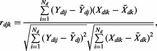
Various methods, such as correlation, regularized regression and Bayesian modeling, can be used to infer interactions in a single cancer. Given the assumption that miRNAs and target gene expression are negatively correlated, the most straightforward method is through the Pearson correlation on pre-processed (standardized and/or normalized) expression data. Although regularized regression and Bayesian modeling can deal with collinearity issues among miRNAs and provide a sparse solution with variable selection, a number of studies indicate that miRNA families with members of high-sequence identity and miRNA clusters classified by genomic locations may present coexpression patterns and regulate genes cooperatively (Chhabra et al., 2010; Cloonan et al., 2011; Xiao et al., 2012). Therefore, some true interactions might be incorrectly excluded by sparse solutions among correlated miRNAs. Moreover, sparse solutions may choose different sets of interaction pairs for each cancer when there is a strong correlation among miRNAs and genes, leading to potential issue of ‘missing data’ when joint analysis is performed across cancers. Thus, we have chosen to use Pearson correlation (Equation 1) to quantify the statistical evidence of association between miRNAs and genes in each cancer. The statistical significance level is calculated by Fisher transformation (Equation 2), an approximate variance-stabilizing transformation, which follows a normal distribution.
 |
(1) |
| (2) |
where  is the Pearson correlation coefficient between gene j and miRNA k in disease d;
  is the expression of gene j in individual i of disease d;
  is the expression of miRNA k in individual i of disease d;
  is the number of individuals in disease d;
  is the z-score of each pair gained from the Fisher transformation of the Pearson correlation coefficient.
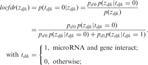
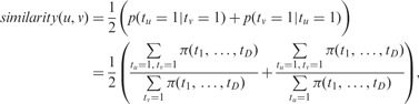
To estimate the probabilities of interactions within each cancer, the local false discovery rate (abbreviated as local fdr in the following) estimation procedure developed by Efron (2004) was used to simultaneously consider all miRNA–gene interactions. Local fdr is an empirical Bayes method suitable for large-scale hypothesis testing involving many hypotheses, and it performs well when most of the cases belong to the null distribution and the test statistic under the null distribution is approximately normally distributed. The local fdr estimates the empirical null distribution from the central peak in the z-values’ histogram, which is preferred over permutation-based null distribution estimation when dilation effects (unobserved covariates) are present (Efron, 2004). The local fdr method fits well for the miRNA–gene interaction analysis, as most miRNA and gene pairs do not interact, the z-scores calculated from Equation (2) approximately follow a normal distribution and unobserved covariates are universal in biological studies. The local fdr for each miRNA–gene within a cancer is estimated by:
 |
(3) |
where  is an indicator variable representing whether a gene j and miRNA k interact;
  is the probability of null cases (no interaction); and
  is the probability of non-null cases (true interactions).
Then the probability of interaction given its z-score is estimated through the following Equation:
| (4) |
For a set of Z-values,  can be estimated from R package ‘locfdr’, based on the local fdr method. With the Pearson correlation, Fisher transformation and local fdr estimation, we infer the probabilities of interactions within each cancer, given the expression dependency between genes and miRNAs.
2.1.2 Inference of cross-cancer pairs probability
In the first stage analysis as discussed earlier in the text, miRNA–gene interactions are studied in cancers individually. Therefore, shared information across multiple cancers is not taken into account. In the second stage, we jointly analyze multiple cancers with an empirical Bayes approach to effectively incorporate shared information to identify interactions. The ultimate goal of this joint analysis is to estimate the probability of interactions in cancer d given the z-scores of all cancers  .
.
In our following discussion, multiple studies refer to different cancers that may have distinct miRNA regulatory networks. Therefore, it is expected that only a fraction of the interactions is shared among cancers. In addition, we expect that cancers that are more closely related (e.g. ovarian cancer and breast cancer) should have a higher degree of sharing than those that are more distantly related. In other words, the joint miRNA–gene interaction patterns across cancers are dependent on both the interaction probabilities in each individual cancer (derived in Section 2.1.1) and the overall similarity of miRNA regulatory networks across cancers. To quantify the overall similarity, the most straightforward way is to calculate the fraction of miRNA–gene pairs shared between two cancers. The rationale can be formulated as follows. Let  denote the joint interaction status among cancers for a study of D cancers with
  representing the status of interaction in cancer d. As
  could be either 1 or 0, the joint status of D cancers has 2D possible patterns. For example, there are eight joint patterns (0,0,0), (0,0,1), (0,1,0), (1,0,0), (0,1,1), (1,0,1), (1,1,0) and (1,1,1) for three cancers under study. Let
  denote the probability for pattern
  . The overall similarity of miRNA regulation between cancers u and v (
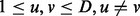 ) can be quantified by the fraction of shared pairs from
  by Equation (5).
 |
(5) |
Thus, the interactions common across cancers, which are shown by the overall similarity, can be incorporated into the joint estimation of pairs via the probability for each interaction pattern  . In our algorithm, we use
  to implicitly represent the overall similarity, considering indirectly using the similarity scores in the study.
Then, we consider combining the probability of individual cancers with similarity [via  ] for inference of interactions. Although z-scores of the pairs are not independent among cancers because of the shared information, we assume conditional z-scores of a pair in different cancers are independent when the status of interactions for each cancer is known; therefore, the probability of observing z-scores given the interaction status is:
| (6) |
With  obtained from local fdr estimation in the first stage, we have
 |
(7) |
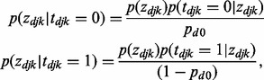
By combining the estimated probabilities in individual cancers and estimation of similarity among cancers, we can derive the posterior marginal probability of interaction between gene j and miRNA k given observed z-scores.
 |
(8) |
The only unknown parameters in Equation (8) are the prior probabilities  , which measure cancer similarities. We empirically estimate
  from the observed data with an iterative updating algorithm shown in Figure 1. Because only the negative relationship is considered for miRNA–gene interactions, we assign
 if
if  after the iterative inference.
Fig. 1.

Iterative updating algorithm to estimate posterior marginal probabilities for status of interactions with empirically estimated 
2.2 Simulations
To demonstrate the benefit of joint analysis of multiple cancers to infer interaction by the proposed method MCMG, we performed extensive simulations on four scenarios considering the characteristics and issues in miRNA–gene paired expression data. To simulate realistic data for miRNA–gene pairs, both gene and miRNA expression data have to be separately generated and the dependency within and between these two types of data has to be modeled as well. We are not aware of software to perform such simulations in the literature, partly because of the difficulty to mimic the features and dependency of miRNA–gene pairs. Thus, in our studies, we directly simulated the transformed correlation coefficients between miRNAs and genes from Gaussian mixture distributions (z-values’ distribution of miRNA–gene pairs in one cancer) to mimic the output of single cancer analysis. The main goal of our simulations was to demonstrate the advantage of joint analysis of multiple cancers over single cancer analysis. To better incorporate the characteristics of miRNA–gene data, we simulated pairs from Gaussian mixture distributions with different separation of null and non-null parts, different similarity among cancers, and with or without pairs of positive correlations (details discussed below). In each scenario, 10 000 miRNA–gene pairs were simulated with 10 repeats. We assumed that 90% of the pairs had no interactions, i.e.  = 0.9, whereas there were interactions between for the other 10%, e.g.
  = 0.1, in cancer d. When there was no interaction, we assumed that
  . Let D denote the number of cancers. We considered the following four scenarios in our simulations.
Scenario I: We studied the effect of separation of null and alternative distributions in individual cancers. Because miRNAs and genes are assumed to be negatively correlated, we assumed that the alternative distribution is a normal distribution with a negative mean,
 for two cancers where they share the same set of interacting miRNA–gene pairs.
Scenario II: We studied the effect of similarity of interaction sets among cancers. We expect that our method performs better with more overlaps of interactions among cancers. We assessed the performance of our proposed method when two cancers shared 60, 70, 80, 90 or 100% of interacting sets.
Scenario III: We studied the effect of the number of cancers included in the study. We expect that our proposed method performs better when more cancers are jointly analyzed together. We varied the number of cancers considered from 2, 4, to 6.
Scenario IV: We studied the effect of positive correlations between miRNAs and their target genes. Although most miRNA–gene interactions are negative, positive correlations have been observed in difference cancers because of specific biological reasons, e.g. downstream genes in the pathway regulated by miRNA or close physical locations (Creighton et al., 2012). To assess their effect on interaction inference, we let alternative distributions consist of two parts,
 , in a study involving two cancers. The non-null cases were simulated from these two distributions with equal chance.
The precision-recall curves [Equation (9)] were used to evaluate the performance of the proposed method by comparing results from analyzing single cancers individually and analyzing multiple cancers jointly. The precision-recall curves were plotted based on the average of 10 simulated datasets for each scenario. In our simulation, some existing approaches to studying miRNA–gene interactions, such as Lasso and GenMir++, are not applicable because they require expression profiles and are limited to single cancer analysis or simple aggregate analysis.
 |
(9) |
2.3 Real data analysis
We considered TCGA datasets with large sample sizes that enable us to study the miRNA–gene interactions individually and jointly. At the time of our analysis, a few cancer datasets, including OV, GBM and BRCA, were available for use without restrictions. At least 400 tumor samples in each cancer were profiled for paired miRNA and gene expressions using different platforms. OV and GBM were studied by expression microarrays; BRCA was studied by RNA-seq and miRNA-seq. These three cancers were used to evaluate MCMG for joint inference of miRNA–gene interactions.
For microarray datasets, the level 3 summarized data were downloaded, and then batch effects were corrected with combat (Johnson et al., 2007) for both gene and miRNA expression levels. For RNA-seq and miRNA-seq datasets, the level 3 data with reads per kilobase per million (RPKM) normalization were downloaded. Then for the miRNA or gene expression matrix in one cancer, the sample median was subtracted, and then genes and miRNAs with high variability were selected by median absolute deviation ≥0.4 as done in the original TCGA publications (The Cancer Genome Atlas Network, 2011). Then quantile normalization was applied to each gene or miRNA across samples to facilitate correlation analysis. The selected genes and miRNAs overlapped among cancers are subjected to subsequent analysis of interaction identification.
The performance of our proposed method, MCMG, was compared with the existing methods to infer miRNA–gene interactions from expression datasets. The representative methods we compared include the Pearson correlation in the simple correlation analysis category, Lasso regression (Lu et al., 2011) in the simple/regularized regression category and GenMir++ (Huang et al., 2007) in the Bayesian inference category. Because the existing methods cannot perform joint analysis, they were applied both to individual cancers and simple aggregate datasets (concatenate all cancer data together to form one set).
3 RESULTS AND DISCUSSION
3.1 Simulation studies
To assess the effectiveness of MCMG, we performed four sets of simulations as described in the ‘Methods’ section.
We first considered a simple biological setting where the two cancers shared the same set of miRNA–gene pairs and investigated the effect of interaction strengths on the performance of our method. We assumed the mean values for the alternative distribution to be −1, −2 and −3, respectively. The estimation of the probability of the null distribution ( ) was 0.995 (Fig. 2A), 0.961 (Fig. 2B) and 0.916 (Fig. 2C), respectively, by the maximum likelihood estimation, where the true
  was 0.9. The estimation of
  is more accurate with larger separations. In Figure 2D, the precision-recall curves show that the joint analysis improved the detection of true interactions under all mean values of non-null distribution even when the true interactions were not able to be well-distinguished from the null distribution as
  . The greatest improvement was achieved by
  , as a larger separation such as
  is already sufficient to identify the majority of true interactions with single cancer analysis. Thus, in the following simulations, we used
  to estimate the benefit of joint inference of multiple cancers.
Fig. 2.
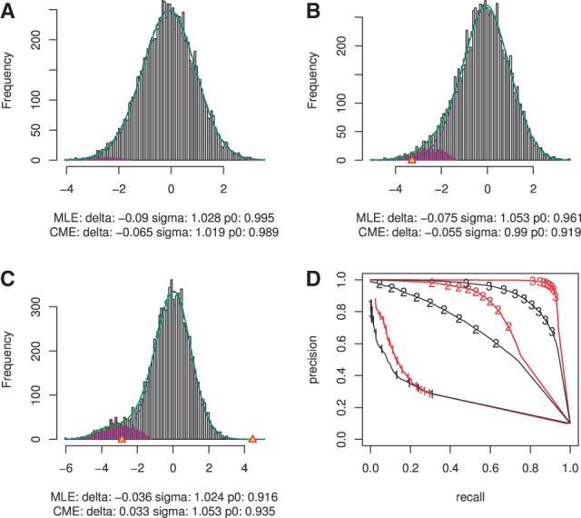
The effect of separation of null and alternative distributions (scenario I). (A-C) Local FDR estimation of data with alternative distribution mean −1, −2 and −3. (D) Precision-recall curve for three mean values. Black lines represent single cancer analysis and red lines represent joint analysis of multiple cancers, labeled with number 1, 2 and 3 for mean value −1, −2 and −3, respectively
The second set of simulations explored the effect of similarity (the proportion of overlapping interaction sets) among cancers. The underlying idea of MCMG is to integrate commonality among cancers to increase the power of detection of true interactions and reduce false-positive results. So we expect a higher number of shared interactions among cancers would enhance the accuracy of posterior probability estimation from single cancer analysis. This was the case as shown in Figures 3A–C with different numbers of cancers studied, which indicates that MCMG can capture the shared information well. In addition, Figure 3 also reveals that more different but related cancers involved in joint analysis provide the opportunity to compensate the interaction heterogeneity among each other, which results in a higher power to discover true positives. Specifically, different interactions may be shared by different groups of cancers under study. More cancer types present in a joint study offer greater shared information available on interactions, leading to improved inference. Then, we used probabilities of status  to calculate the similarities as shown in Equation (5). The estimated similarities have a linear relationship with true similarities, but ∼10–20% lower than the true ones considering the absolute values (Fig. 3D). It might be mainly because of the difficulty to classify the pairs at the boundary of null and alternative distributions. But the accurate estimation of the similarity trend would help MCMG to put correct ‘weights’ [
 ] among cancers to infer interactions.
Fig. 3.
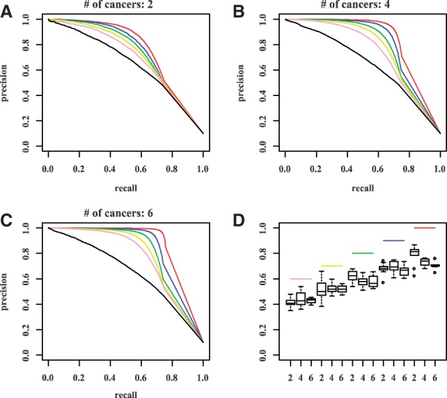
The effect of similarity of interaction sets among cancers (scenario II) and number of cancers in the joint study (scenario III). (A-C) Precision-recall curves for different similarities among cancers and different number of cancers (A:2, B:4, C:6) involved in study. Black lines represent single cancer analysis; colored lines represent joint analysis with different similarities among cancers. Red: 100%; blue: 90%; green: 80%; yellow: 70%; pink: 60%. D. True and estimated similarity among cancers by joint analysis of 2, 4 and 6 cancers. Colored lines are true similarity levels; boxplots show the corresponding estimation from 10 repeats
In the last scenario, we examined an effect that is specific and inevitable in miRNA studies, namely, the presence of positive correlations (∼5% of all pairs) between miRNA and their targets. The systematic positive correlations may increase the posterior probability for some false interactions. In this simulation, the effect of systematic positive correlations was investigated to see whether these ‘unwanted’ correlations would affect the prediction of true sets. The precision-recall curves were just slightly lower compared with those of negative true sets only (Fig. 3A), and the improvement of prediction was still obvious (Fig. 4), suggesting that the presence of high positive z-scores may not affect the performance of the method. The standard deviation of precision and recall calculated in all scenarios ranges from 0 to 0.04 with a median of ∼0.02, which shows the stability of the methods on interaction discovery among repeats in the simulations.
Fig. 4.
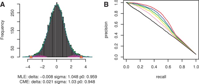
The effect of systematic high positive correlations among cancers (scenario IV). (A) Local FDR estimation on the dataset with both negative and positive correlations of miRNAs and genes. (B) Precision-recall curves for different similarities among cancers. Black lines represent single cancer analysis; colored lines represent joint analysis with different similarity among cancers. Red: 100%; blue: 90%; green: 80%; yellow: 70%; pink: 60%
3.2 Real data application
In this section, we demonstrate the effectiveness of the proposed method on miRNA–gene interaction identification using TCGA datasets. First, expression profiles of two cancers generated with the same technique (gene expression microarray) were used to show the improvement of inference. Then, we incorporated another cancer studied by RNA-seq to illustrate the analysis of three cancers and the ability of our method to naturally incorporate different data types in interaction inference.
3.2.1 Two cancers with the same data type
We first considered paired expression profiling of OV and GBM. In total, 4698 genes and 119 miRNAs with high variability among samples were selected. The estimation of the probability of null distribution  was 0.919 and 0.871 for OV and GBM, respectively. The fact that the estimated
  was close to 0.9 suggested that a substantial fraction (∼10%) of pairs may interact, despite some non-null pairs may be contributed by the heterogeneity of samples in one cancer. The proposed method converged after 20 iterations with the probabilities of joint status (OV, GBM) (0,0), (0,1), (1,0) and (1,1) estimated to be 0.829, 0.056, 0.0532 and 0.0619, respectively. The similarity of miRNA regulatory genes between OV and GBM was estimated to be 53.14% by Equation (5). Because our method may underestimate the similarity between cancers as suggested in simulation scenarios II and III (Fig. 3) due to ambiguous pairs at boundaries, the true similarity between these two cancers may be higher.
To visualize how joint analysis impacts the inferred interaction pairs compared with single cancer analysis, Figure 5A and B for OV and GBM compared the inferred probabilities from within-cancer and cross-cancer analysis to z-scores from the Pearson correlation. Within-cancer inference, which was calculated from the Fisher transformed correlation and followed by local fdr estimation, did not change the order of z-scores, but cross-cancer inference did lead to a different priority of interactions because of the joint analysis of multiple cancers. Therefore, joint inference using data from two cancers clearly re-prioritized candidate miRNA–gene interactions through incorporating shared information among cancers.
Fig. 5.
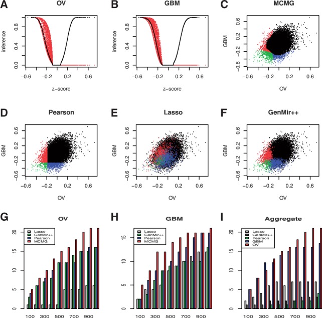
Real data application on OV and GBM. (A-B) z-scores from Pearson correlation and Fisher transformation versus the probability inference of interactions within cancers (black dots) and across cancers (red dots) in OV (A) and GBM (B). (C-F) Visualization of top 1000 interactions selected by MCMG (C), Pearson correlation (D), Lasso (E) and GenMir++ (F). X and Y axis’s represent z-score from OV and GBM, respectively. Red ones are selected by OV only; blue are selected by GBM only; green are selected by both cancers. (G-I) The number of validated targets selected by different methods at 10 cutoffs of top list (top 100 to 1000 with 100 interval). For comparison methods, G: single cancer analysis of OV; H: single cancer analysis of GBM; I: simple aggregate dataset combining OV and GBM. For MCMG, all results are from joint analysis. The ‘OV’ and ‘GMB’ in (I) represent the results from MCMG. For some cutoffs, methods may show higher number of predicted interactions than the value of cutoff when several pairs have identical scores, so we rescaled the number of validated interactions to make sure the cutoff values are the same across methods
To show that joint analysis led to improved inference of interactions, the results from MCMG were compared with those from three representative approaches with single cancer analysis and/or simple aggregate analysis, including the Pearson correlation, Lasso (Lu et al., 2011) and GenMir++ (Huang et al., 2007), which were proven to enrich the signals compared with sequence-based prediction. MCMG jointly analyzed multiple cancers, whereas three existing methods were applied both to individual cancers and simple aggregates of both cancer datasets because these methods are not able to perform joint analysis. We focused on the 21 806 miRNA–gene pairs that were predicted by TargetScan V6.1 (Lewis et al., 2005) for method comparison because other methods performed the selection within predicted interaction sets as designed in their original articles. It is likely that different cancers may share common miRNA–gene interactions because miRNAs globally regulate genes in tissues and developmental stages. This is the assumption underlying both the analysis of aggregated dataset and our proposed method. Thus, the first comparison was to examine how each method identified common and specific interactions for two cancers (Fig. 5C–F). By considering the top 1000 interactions predicted by each method, the Pearson correlation (Fig. 5D) just set the hard cutoff at z-score around −0.2 for selection, which identified 203 common interactions between OV and GBM. The other three approaches, including Lasso, GenMir++ and our proposed method, prioritized the interactions differently, and we observed great differences between these three methods and the naïve correlation method. As expected, our proposed method was able to identify the largest number of common pairs (614 pairs) by integrating shared information (Fig. 5C). By considering the commonality of miRNA regulatory mechanisms, the joint analysis stage of MCMG with the empirical Bayes method provided valuable information to prioritize interactions seen in two cancers over the ones found in only one when they have similar z-scores. Meanwhile, our method still identified miRNA–gene interaction pairs (396 pairs) specific for each cancer that account for the heterogeneity among cancers. GenMir++ identified 204 common pairs (Fig. 5F), similar to the Pearson correlation (Fig. 5D), whereas Lasso only identified 127 common ones and some of them even had z-scores near 0 (Fig. 5E). The reason might be that the pairs in Lasso were ranked with a refined score from 100 to 0 based on estimated regression coefficient in each gene separately. The ranking method might be good if multiple diseases are combined to find pairs because more sets of genes might be involved in miRNA regulation processes. However, here we studied cancers separately, and the ranking method may select some pairs from genes not involved in the miRNA regulation in the cancer, which results in high ranking but with small z-values.
To further evaluate the performance of the proposed method, we examined the number of validated interactions identified in the top of the target lists by each method in OV (Fig. 5G) and GBM (Fig. 5H). Among predicted ones by TargetScan, 72 were experimentally validated and curated by TarBase V5.0 (Papadopoulos et al., 2009). Enrichment of validated targets is improved by all methods incorporating expression data compared with the sequence-based prediction-only method TargetScan. The Pearson correlation and GenMir++ had a similar number of validated targets at different cutoffs. The Lasso method did not perform well in OV, but had similar performance in GBM. However, MCMG showed consistently better identification of validated targets in every cutoff in this two-cancer study.
The comparison methods can be applied to aggregated datasets concatenating the two cancers together. We applied the Pearson correlation, Lasso and GenMir++ to concatenated OV and GBM data (Fig. 5I). Probably because of the refined scores provided by the Lasso method for each gene separately, Lasso performed better than the other two methods in the situation of aggregated dataset when more genes might be involved in the miRNA regulatory network than that of a single cancer dataset. However, all comparison methods identified fewer validated targets than those identified by the analysis of single cancers. So MCMG had even better performance here because it already showed enhanced identification of pairs compared with single cancer analysis in Figure 5G and H. Higher accuracy of single cancer analysis compared with simple aggregate analysis also confirmed the hypothesis that when the sample size is sufficiently large, single cancer analysis would be preferred.
3.2.2 Three cancers with different data types
Next, we considered joint analysis of three cancers (OV, GBM, BRCA) collected on different platforms, where BRCA was generated by RNAseq, whereas the other two were measured by microarrays. These three datasets are not able to be concatenated because of their different formats, so the existing methods can only be applied to single cancer analysis, but not aggregate analysis. However, our method can naturally incorporate different data types to infer interacting miRNA–gene pairs. The within-cancer inference step generates normalized z-scores for all cancers no matter what the data type is, and then there is no difficulty to apply the second stage cross-cancer inference of MCMG to well-formatted z-scores.
The estimated probabilities converged after 26 iterations for the joint status (OV, GBM, BRCA): 0.7282, 0.0971, 0.0532, 0.0198, 0.0169, 0.0287, 0.0207 and 0.0355, for (0,0,0), (0,0,1), (0,1,0), (0,1,1), (1,0,0), (1,0,1), (1,1,0) and (1,1,1), respectively. The similarity between OV and BRCA was estimated to be 49.26%, which was higher than the 36.66% estimated between GBM and BRCA, showing closer relationship of OV and BRCA than GBM and BRCA. Despite the 49.36% similarity score between OV and GBM, the percentage of shared interactions of OV-GBM and OV-BRCA in all the potential interaction list of OV was 56.16 and 64.19%, which agreed with the conclusion that the estimated similarity of OV and BRCA is higher than GBM and BRCA. This is consistent with our expectation that BRCA and OV are more similar among the three cancers because they are both female cancers and share some commonality in cancer-causing mutations or pathways (The Cancer Genome Atlas Network, 2012). Thus, MCMG led to a reasonable similarity inference among cancers based on gene–miRNA interaction data.
The number of validated interactions in the top lists was also investigated for the three-cancer study. The results of OV (Fig. 6A) and GBM (Fig. 6B) are similar to those from the joint analysis of two cancers, as our method can identify the largest number of validated interactions from predicted ones. For BRCA (Fig. 6C), Lasso had better prediction than Pearson and GenMir++. But our proposed method was still the best among all methods from the top list 200–1000.
Fig. 6.
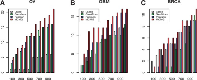
Real data application on three cancer datasets, OV, GBM and BRCA. The number of validated targets selected by different methods at 10 cutoffs of top list (top 100 to 1000 with 100 interval) for OV (A), GBM (B) and BRCA (C). For some cutoffs, methods may show more number of predicted interactions than the value of cutoff when several pairs have the identical scores, so we rescaled the number of validated interactions to make sure the cutoff values are the same across methods
Thus, real data analyses showed that our method outperformed existing methods by taking into account shared information and provided good assessment of relationship among cancers.
4 CONCLUSION
The existing analysis of miRNA–gene interactions with expression data is either based on a single cancer dataset or an aggregated dataset concatenated from multiple cancers. In this article, we proposed a novel approach (MCMG) to study microRNA–gene interactions with paired expression profiles. We use an empirical Bayes method to explicitly borrow information among cancers to improve the identification of interactions. With simulation studies considering features of gene–miRNA pair data and two sets of real TCGA data analysis, we demonstrated the benefit of our joint analysis compared with single cancer or simple aggregate analysis. MCMG can efficiently recognize common interactions, and also retains specific miRNA regulations for each cancer. Interestingly, the hidden relationship among cancers could also be quantitatively estimated by our method based on miRNA–gene pairs data, which might be useful for other disease studies as well. This two-stage method infers the probability of interactions within each cancer and then the posterior marginal probability considering all cancers in a sequential manner, which enables us to naturally combine cancers with different data types in the study. The two-stage design also provides the possibility to substitute the initial step (Pearson correlation) with results from other methods (such as Lasso or Bayesian inference) if one prefers, and then they can still benefit from the second stage of integrating multiple cancers for better prediction.
ACKNOWLEDGEMENTS
We thank Xiu Huang, John Ferguson and Can Yang for helpful discussions, and Yale University Biomedical High Performance Computing Center (YHPC) for data storage and computation runs.
Funding: XC was supported by Lo Graduate Fellowship for Excellence in Stem Cell Research and a fellowship from the China Scholars Council. FJS was supported by National Institutes of Health (grant no. CA131301) and an Anonymous Foundation. HZ was supported by National Institutes of Health (grant no. NIH R01 GM59507 and P01CA154295) and National Science Foundation (grant no. NSF DMS 1106738). YHPC was funded by National Institutes of Health (grant no. NIH RR19895).
Conflict of Interest: none declared.
REFERENCES
- Anvar SY, et al. Interspecies translation of disease networks increases robustness and predictive accuracy. PLoS Comput. Biol. 2011;7:e1002258. doi: 10.1371/journal.pcbi.1002258. [DOI] [PMC free article] [PubMed] [Google Scholar]
- Bartel DP. MicroRNAs: genomics, biogenesis, mechanism, and function. Cell. 2004;116:281–297. doi: 10.1016/s0092-8674(04)00045-5. [DOI] [PubMed] [Google Scholar]
- Chen Y, et al. MM-ChIP enables integrative analysis of cross-platform and between-laboratory ChIP-chip or ChIP-seq data. Genome Biol. 2011;12:R11. doi: 10.1186/gb-2011-12-2-r11. [DOI] [PMC free article] [PubMed] [Google Scholar]
- Chhabra R, et al. Cooperative and individualistic functions of the microRNAs in the miR-23a∼27a∼24-2 cluster and its implication in human diseases. Mol. Cancer. 2010;9:232. doi: 10.1186/1476-4598-9-232. [DOI] [PMC free article] [PubMed] [Google Scholar]
- Choi H, et al. Sparsely correlated hidden Markov models with application to genome-wide location studies. Bioinformatics. 2013;29:533–541. doi: 10.1093/bioinformatics/btt012. [DOI] [PMC free article] [PubMed] [Google Scholar]
- Choi H, et al. Hierarchical hidden Markov model with application to joint analysis of ChIP-chip and ChIP-seq data. Bioinformatics. 2009;25:1715–1721. doi: 10.1093/bioinformatics/btp312. [DOI] [PMC free article] [PubMed] [Google Scholar]
- Cloonan N, et al. MicroRNAs and their isomiRs function cooperatively to target common biological pathways. Genome Biol. 2011;12:R126. doi: 10.1186/gb-2011-12-12-r126. [DOI] [PMC free article] [PubMed] [Google Scholar]
- Creighton CJ, et al. Integrated analyses of microRNAs demonstrate their widespread influence on gene expression in high-grade serous ovarian carcinoma. PLoS One. 2012;7:e34546. doi: 10.1371/journal.pone.0034546. [DOI] [PMC free article] [PubMed] [Google Scholar]
- Datta D, Zhao H. Statistical methods to infer cooperative binding among transcription factors in Saccharomyces cerevisiae. Bioinformatics. 2008;24:545–552. doi: 10.1093/bioinformatics/btm523. [DOI] [PubMed] [Google Scholar]
- De Jager PL, et al. Meta-analysis of genome scans and replication identify CD6, IRF8 and TNFRSF1A as new multiple sclerosis susceptibility loci. Nat. Genet. 2009;41:776–782. doi: 10.1038/ng.401. [DOI] [PMC free article] [PubMed] [Google Scholar]
- Efron B. Large-scale simultaneous hypothesis testing: the choice of a null hypothesis. J. Amer. Statist. Assoc. 2004;99:9. [Google Scholar]
- Enright AJ, et al. MicroRNA targets in Drosophila. Genome Biol. 2003;5:R1. doi: 10.1186/gb-2003-5-1-r1. [DOI] [PMC free article] [PubMed] [Google Scholar]
- Esquela-Kerscher A, Slack FJ. Oncomirs - microRNAs with a role in cancer. Nat. Rev. Cancer. 2006;6:259–269. doi: 10.1038/nrc1840. [DOI] [PubMed] [Google Scholar]
- Ferguson JP, et al. A new approach for the joint analysis of multiple ChIP-seq libraries with application to histone modification. Stat. Appl. Genet. Mol. Biol. 2012;11:Article 1. doi: 10.1515/1544-6115.1660. [DOI] [PMC free article] [PubMed] [Google Scholar]
- Ferrucci L, et al. Common variation in the beta-carotene 15,15'-monooxygenase 1 gene affects circulating levels of carotenoids: a genome-wide association study. Am. J. Hum. Genet. 2009;84:123–133. doi: 10.1016/j.ajhg.2008.12.019. [DOI] [PMC free article] [PubMed] [Google Scholar]
- Huang JC, et al. Using expression profiling data to identify human microRNA targets. Nat. Methods. 2007;4:1045–1049. doi: 10.1038/nmeth1130. [DOI] [PubMed] [Google Scholar]
- Johnson WE, et al. Adjusting batch effects in microarray expression data using empirical Bayes methods. Biostatistics. 2007;8:118–127. doi: 10.1093/biostatistics/kxj037. [DOI] [PubMed] [Google Scholar]
- Kim S, et al. Identifying the target mRNAs of microRNAs in colorectal cancer. Comput. Biol. Chem. 2009;33:94–99. doi: 10.1016/j.compbiolchem.2008.07.016. [DOI] [PubMed] [Google Scholar]
- Krek A, et al. Combinatorial microRNA target predictions. Nat. Genet. 2005;37:495–500. doi: 10.1038/ng1536. [DOI] [PubMed] [Google Scholar]
- Lewis BP, et al. Conserved seed pairing, often flanked by adenosines, indicates that thousands of human genes are microRNA targets. Cell. 2005;120:15–20. doi: 10.1016/j.cell.2004.12.035. [DOI] [PubMed] [Google Scholar]
- Lewis BP, et al. Prediction of mammalian microRNA targets. Cell. 2003;115:787–798. doi: 10.1016/s0092-8674(03)01018-3. [DOI] [PubMed] [Google Scholar]
- Liu B, et al. Exploring complex miRNA-mRNA interactions with Bayesian networks by splitting-averaging strategy. BMC Bioinformatics. 2009;10:408. doi: 10.1186/1471-2105-10-408. [DOI] [PMC free article] [PubMed] [Google Scholar]
- Liu H, et al. Identifying mRNA targets of microRNA dysregulated in cancer: with application to clear cell Renal Cell Carcinoma. BMC Syst. Biol. 2010;4:51. doi: 10.1186/1752-0509-4-51. [DOI] [PMC free article] [PubMed] [Google Scholar]
- Lu Y, et al. A Lasso regression model for the construction of microRNA-target regulatory networks. Bioinformatics. 2011;27:2406–2413. doi: 10.1093/bioinformatics/btr410. [DOI] [PubMed] [Google Scholar]
- Muniategui A, et al. Quantification of miRNA-mRNA interactions. PloS One. 2012a;7:e30766. doi: 10.1371/journal.pone.0030766. [DOI] [PMC free article] [PubMed] [Google Scholar]
- Muniategui A, et al. Joint analysis of miRNA and mRNA expression data. Brief. Bioinform. 2012b;14:263–278. doi: 10.1093/bib/bbs028. [DOI] [PubMed] [Google Scholar]
- Papadopoulos GL, et al. The database of experimentally supported targets: a functional update of TarBase. Nucleic Acids Res. 2009;37:D155–D158. doi: 10.1093/nar/gkn809. [DOI] [PMC free article] [PubMed] [Google Scholar]
- Sethupathy P, et al. A guide through present computational approaches for the identification of mammalian microRNA targets. Nat. Methods. 2006;3:881–886. doi: 10.1038/nmeth954. [DOI] [PubMed] [Google Scholar]
- Soranzo N, et al. Meta-analysis of genome-wide scans for human adult stature identifies novel Loci and associations with measures of skeletal frame size. PLoS Genet. 2009;5:e1000445. doi: 10.1371/journal.pgen.1000445. [DOI] [PMC free article] [PubMed] [Google Scholar]
- Steele E, Tucker A. Consensus and Meta-analysis regulatory networks for combining multiple microarray gene expression datasets. J. Biomed. Inform. 2008;41:914–926. doi: 10.1016/j.jbi.2008.01.011. [DOI] [PubMed] [Google Scholar]
- Stingo FC, et al. A Bayesian graphical modeling approach to microRNA regulatory network inference. Ann. Appl. Stat. 2010;4:25. doi: 10.1214/10-AOAS360. [DOI] [PMC free article] [PubMed] [Google Scholar]
- Su N, et al. Predicting MicroRNA targets by integrating sequence and expression data in cancer. IEEE Int Conf Syst Biol. 2011 [Google Scholar]
- The Cancer Genome Atlas Network. Integrated genomic analyses of ovarian carcinoma. Nature. 2011;474:609–615. doi: 10.1038/nature10166. [DOI] [PMC free article] [PubMed] [Google Scholar]
- The Cancer Genome Atlas Network. Comprehensive molecular portraits of human breast tumours. Nature. 2012;490:61–70. doi: 10.1038/nature11412. [DOI] [PMC free article] [PubMed] [Google Scholar]
- The Cancer Genome Atlas Research Network. Comprehensive genomic characterization defines human glioblastoma genes and core pathways. Nature. 2008;455:1061–1068. doi: 10.1038/nature07385. [DOI] [PMC free article] [PubMed] [Google Scholar]
- Van der Auwera I, et al. Integrated miRNA and mRNA expression profiling of the inflammatory breast cancer subtype. Br. J. Cancer. 2010;103:532–541. doi: 10.1038/sj.bjc.6605787. [DOI] [PMC free article] [PubMed] [Google Scholar]
- Xiao Y, et al. Discovering dysfunction of multiple microRNAs cooperation in disease by a conserved microRNA co-expression network. PloS One. 2012;7:e32201. doi: 10.1371/journal.pone.0032201. [DOI] [PMC free article] [PubMed] [Google Scholar]