Massively Parallel MRI Detector Arrays

Abstract

Originally proposed as a method to increase sensitivity by extending the locally high-sensitivity of small surface coil elements to larger areas, the term parallel imaging now includes the use of array coils to perform image encoding. This methodology has impacted clinical imaging to the point where many examinations are performed with an array comprising multiple smaller surface coil elements as the detector of the MR signal. This article reviews the theoretical and experimental basis for the trend towards higher channel counts relying on insights gained from modeling and experimental studies as well as the theoretical analysis of the so-called “ultimate” SNR and g-factor. We also review the methods for optimally combining array data and changes in RF methodology needed to construct massively parallel MRI detector arrays and show some examples of state-of-the-art for highly accelerated imaging with the resulting highly parallel arrays.

Introduction

The past decade of Magnetic Resonance Imaging (MRI) has seen tremendous advances toward improved sensitivity and reduced scan-time in clinical and research imaging examinations. While gradient performance improvements in strength and slew-rate always played an important role in terms of acquisition speed, magnet field strength and well-crafted detector geometries have always been critical for maximizing the sensitivity of the MR experiment. Because of this important role of a coil detector in determining sensitivity, we focus on receive arrays; although we note that transmit arrays have recently become an object of study in their own right [1–7].

Roemer and colleagues [8] showed that simultaneous detection of the MR signal with an array of surface coils could out-perform a single, larger surface coil covering the same area and gave a detailed description of how to optimally combine the data from the multiple elements given their sensitivity profile and measured noise correlation information. They further introduced the concept of “preamplifier decoupling” to suppress inductive coupling within the array using low-input impedance preamplifiers [8]. Only a year later, this concept was extended to volume-like acquisitions to show that the sensitivity of the array could compete favorably with volume coils [9]. While the spine was Roemer’s initial focus and a logical place to distribute the reception coils along the length of the body, the concept was quickly extended to imaging other parts of the body [9–13] and to spectroscopy applications [14,15]. Interestingly, the brain, with its nearly spherical geometry was a less obvious target for arrays, and was among the last applications [16–18].

These demonstrations alone were enough to make array coils the favored method for many types of MRI examinations. But a second advantage of detection with arrays was soon introduced; namely the ability to reconstruct under-sampled k-space data and thus significantly speed up the MR image encoding process. These parallel imaging reconstruction techniques effectively used the additional spatial information contained in the signal intensity and phase profiles of the array elements to allow reconstruction of the image from under-sampled k-space data sets. In these methods, the image encoding is shared by the array coil and the gradient encoding steps. It is interesting to note that most imaging modalities rely exclusively on detector arrays for image encoding. For example CCD cameras, EEG and MEG, rely on a dense array of detectors, as does the human eye (where the retina is viewed as an array of photo-detectors), and perhaps most intriguing, the insect eye, which consists entirely of a directionally sensitive array of light-pipes with a few photo-detector cells inside (ommatidia). Medical imaging modalities such as MRI are the outliers where the role of detection and encoding can be completely separated. However, early MR researchers began to realize that the multiple elements could play a role in image encoding [19–23]. While this early work provided glimpses of what could be done, it was only after Roemer’s work propelled the wide-spread implementation of parallel reception that the time was right for incorporating the spatial information present in the array to augment gradient encoding. The fact that the two types of encoding could be merged elegantly, as shown by the introduction of SMASH [24] and SENSE [25] in the late ‘90s, opened the floodgate to the variety of robust methods that exist today.

As a result of the sensitivity increase and encoding acceleration, virtually every clinical coil sold for MRI scanners today is an array. The trend toward higher and higher element counts has also increased over the years; from the initial systems with 4 to 8 elements, to the more commonly used 16 to 32 elements found on most new scanners, to exploration of what can be done with 64 to 128 channels on clinical systems.

In this review, we examine the theoretical basis for the trend toward higher channels from so-called “ultimate SNR” and “ultimate g-factor” analysis, as well as modeling regular geometries. We compare these identified gains to what has been achieved with 32, 64, 96, and 128-channel arrays. We also look at how these trends have forced us to re-think how we tune, match and decouple coils for MR detection. Finally, we look at the trends in MR acquisition sequences which now take advantage of the distribution of coil sensitivity patterns in all three directions.

Optimum combination of individual coil element data

In his original paper, Roemer described a way to elegantly combine the data from the multiple receivers of the array. It is almost always advantageous to combine data obtained from multi-channel array reception in the spatial domain, since the sensitivity profiles of each individual array element can be a steep function of the pixel’s coordinates. Then the optimization can be done on a pixel-by-pixel basis taking into account the spatially changing amplitudes and relative phases of the sensitivity profiles. In addition to measuring the coil signal map S_i(x,y,z) for each element, i, which tells us how the signal vectors will add, we need to know the noise covariance matrix, Ψ, which describes the thermal noise variance in each channel and the covariance between pairs of channels, which informs us of how the noise from the channels adds. For a given pixel, we can form a vector of the coil sensitivity, C, and measured signal level, S, for each channel. Here C and S exist for each pixel and are vectors of length N_ch. We then generate the image intensity, I, of the combined channels for that pixel from a normalized weighted sum of the measured signal levels. The weights will be chosen to maximize the SNR of the combined pixel. We also express the complex weights as a vector, w, of length N_ch. Then the general expression is

$$I=\lambda {\mathbf{w}}^{\mathbf{H}}\mathbf{S},$$ (1)

where λ is a normalization constant which might vary as a function of location but does not effect the pixels SNR. Roemer showed that if the noise variances are equal and uncorrelated (ψ proportional to the identity matrix), then w = C and

$$l=\lambda {\mathbf{C}}^{\mathbf{H}}\mathbf{S}.$$ (2)

To create an image with spatially uniform noise levels, λ is chosen as

$$\lambda ={({\mathbf{C}}^{\mathbf{H}}\mathbf{C})}^{-1/2}$$ (3)

In coil arrays, noise correlations always occurs between channels (either the channel’s variances are unequal, or shared noise or coupling exists in the array). Taking those coupling effects into account, the image combination is fully optimized, when w = Ψ⁻¹C. This results in

$$I^{\text{optSNR}}=\lambda {\mathbf{C}}^{\mathbf{H}}{\mathbf{\Psi }}^{-1}\mathbf{S}$$ (4)

and λ becomes as

$$\lambda ={({\mathbf{C}}^{\mathbf{H}}{\mathbf{\Psi }}^{-1}\mathbf{C})}^{-1/2}.$$ (5)

This can be thought of as “pre-whitening” the signal vector S prior to the combination (replacing S with Ψ⁻¹S). Roemer also showed that if the SNR is high in each channel, then the coil sensitivity vector C is well approximated by the signal vector S and does not need to be measured. I.e. the coil sensitivity is essentially just a map of the signal with perfect SNR. If the noise covariance is also proportional to the identity matrix and we use the λ for uniform noise, then we get what Roemer called the “root sum-of-squares” method;

$$I^{\text{rSoS}}=\sqrt{{\mathbf{S}}^{\mathbf{H}}\mathbf{S}}.$$ (6)

This is a particularly useful form because no pre-scan measurements are required of C or Ψ. One simply takes the sum of the square of the signal levels of each channel’s measurement of that pixel. Since the noise covariance matrix requires only a second to acquire (by digitizing noise in the absence of excitation), it is useful to add this information in, but preserve the estimation of C by S. Then we have the “covariance weighted root-sum-of-squares” combination: I ^cov-rSoS = λ S^H Ψ ⁻¹ S with λ= (S^H Ψ⁻¹ S), which simplifies to

$$I^{cov-\text{rSoS}}=\sqrt{{\mathbf{S}}^{\mathbf{H}}{\mathbf{\Psi }}^{-1}\mathbf{S}}.$$ (7)

Given the choice of weights, w_i, the image SNR is given by [8]:

$$\text{SNR}=\frac{{\mathbf{w}}^{\mathbf{H}}\mathbf{S}}{\sqrt{{\mathbf{w}}^{\mathbf{H}}\mathbf{\Psi }\mathbf{w}}}.$$ (8)

For the other combination methods, the resulting SNR can be shown to be:

$${\text{SNR}}^{\text{rSos}}=\frac{{\mathbf{S}}^{\mathbf{H}}\mathbf{S}}{\sqrt{{\mathbf{S}}^{\mathbf{H}}\mathbf{\Psi }\mathbf{S}}},$$ (9)

while the image SNR for the noise cov-SoS is

$${\text{SNR}}^{cov-\text{rSoS}}=\sqrt{{\mathbf{S}}^{\mathbf{H}}{\mathbf{\Psi }}^{-1}\mathbf{S}}.$$ (10)

Note that the SNR for the covariance weighted sum-of-squares image is (remarkably) the same as the image itself.

In the combination methods above, the complex-valued weights are chosen to maximize the image SNR using the coil sensitivity profiles and noise covariance matrix (or estimates thereof). The problem with the simple noise ROI in the “black” background area of an image is that usually there is no estimate of the coil sensitivities in this region. This results in sub-optimum combination of the array elements in this region and an amplification of the noise by an unknown factor. For example, if the rSoS method is used, the channels are essentially weighted by noise and combined. This is of little concern for discrimination of anatomy, since the weights used inside the body are accurate, but it eliminates this easy method of ROI outside the head to measure noise. Note the ROI in the noise-only part of the image is perfectly valid for single channel coils (after correction for the Rician distribution in magnitude data [26] or if the coil sensitivity is known in that region (for example through a theoretical calculation).

Assessing the SNR of an image acquired with an array coil in a manner that can be readily compared to either another group’s measurements or to the SNR obtained by analyzing the signal mean and variance of a time-series of images requires further considerations. Kellman and McVeigh [27] elegantly described the series of correction factors needed to produce SNR in “absolute units”, which are exactly what is needed to make the calculated SNR maps agree with those obtained from a time-series measurement and subsequently to make SNR maps directly comparable. When these correction factors are used, the SNR measurement some important book-keeping is performed and scale factors accounted for so the SNR maps can be compared from site to site. Four factors are outlined and described in detail. The first defines a “noise equivalent bandwidth” of the receiver, which differs slightly from manufacturer to manufacture and provides a factor that accounts for the “real” bandwidth of the measurement. The second factor accounts for noise averaging by the Fourier Transform by normalizing the noise covariance matrix by the number of samples contributing to the image. The third factor is a simple (2) which arises since the observation model assumes the noise is real valued while the noise is complex valued. The final correction factor, needs to be applied to account for the incorrect assumption of Gaussian noise statistics in magnitude images [10,27,28]. This correction factor applies to the SNR map formed from the rSoS combination, since the individual channels are converted to magnitude maps prior to combination. Then the correction factor is a function of the number of channels and the SNR value thus it must be applied pixel by pixel. It is a generalization of the well-known Rician distribution correction [26] to multichannel rSoS combined arrays, which follow a non-central chi distribution, with 2n degrees of freedom, where n is the number of coils, and is a potentially larger correction [10]. Although often considered unimportant for images with SNR above 10, this correction factor can be significant for highly parallel arrays even for typical SNR levels. For example, the noise statistic bias correction lowers the measured SNR by a factor of 0.6 for a 32-channel acquisition in an image with SNR = 13.

Figure 1 shows the relationship between the naively measured SNR in a rSoS magnitude image and the true SNR. Again, these curves refer to channel combination methods where the magnitude is taken prior to combination, such as the rSoS and the cov-rSoS. If a complex weighting is used (from the coil sensitivity maps), then the complex data is preserved through the coil combination process and if a magnitude operation is applied at the end only the simpler Rician correction needs to be applied (the N_ch =1 curve in Fig. 1) Its also important to note that it not just the SNR that suffers from the elevated mean value of noise regions in the image, but also methods such as high b-value diffusion [29].

Figure 1.

Magnitude detection biases the SNR calculation increasingly with larger coil arrays and increasingly at lower SNR.

Finally, the use of parallel image reconstructions further complicates analysis of image SNR. It introduces spatially-variant noise amplification in the reconstructed images, leading to image SNR degradation associated with the acceleration factor and the coil’s geometry factor (g-factor). The latter has become an attractive figure of merit for assessing the performance of coil arrays for parallel image encoding. While simple methods exist for calculating the noise enhancement in SENSE reconstruction [25], for GRAPPA [30], the equivalent of the g-factor calculation has only been recently addressed [31,32].

SNR in arrays of more and more elements

Here we try to get a feeling for how SNR grows with N_ch for a well-designed array; namely why an array of multiple small coils has higher sensitivity than a single larger coil. It is not surprising that an array of small surface coils does very well near the array compared to a single larger coil or volume coil. But many researchers are surprised that the array can do better (or at least no worse) at all locations, including deep within the tissue. One way to understand this is to consider an array of identical loop detectors tiling a sphere. If all N_ch channels detect the central pixel with equal image intensity and equal levels of uncorrelated noise, then a simple averaging effect occurs when the data is phase-aligned and combined yielding a (N_ch) improvement at the center. This can be a relatively large effect (more than a factor of 10 for a 128-channel array.) But it remains to be seen that this factor is enough to overcome the steep drop-off of the smaller surface coils as a function of depth [33]. The averaging benefit is also reduced in practice since noise correlation necessarily exists even in an inductively decoupled array. In the body-noise dominated case, neighboring coils detect the same noise fluctuations from the random ionic current loops in the lossy tissue if their detection sensitivity patterns overlap, which is nearly always the case for neighboring elements.

Although the intuitive picture suggests that the array can make-up for up to a factor of 10 in sensitivity through the averaging effect, we must turn to modeling to determine if this is enough to out-perform a volume coil or array of larger elements for voxels far from the array. Wiesinger and colleagues [34,35] elegantly answered this through array simulations on a spherical geometry to determine how the SNR of the array grows as a function of the number of channels (N_ch). They also compared the sensitivity to the ultimate SNR performance limit set by Maxwell’s equations for Faraday detection with elements outside the sphere. This is a useful metric since it represents the ideal MR detector (as evaluated with an SNR metric). To calculate the ultimate SNR, a basis set of B₁⁻ sensitivity profiles are used, which i) are solutions to Maxwell’s equations for the geometry of interest, and ii) span the space of solutions to Maxwell’s equations. The latter criterion ensures that any constructed array can be modeled as a linear combination of these basis functions. For example, plane waves can be chosen to model a planar half-space[36,37]. For a spherical phantom, spherical harmonics satisfy the two conditions and can be used as basis vectors [34]. The coil sensitivity patterns of the “ultimate” array must be expressible as a linear combination of these basis vectors. The “ultimate” array is also the one which maximizes SNR at each pixel. This process is done using thousands of elements until the SNR converges to the “ultimate SNR.” Note, that the fact that the array combination method weights each element to optimize SNR, guarantees that adding an element will never lower the SNR; if this were the case, the weight would be zero for that element and, at worst, the SNR is unaffected by the element.

In addition to the ultimate SNR, Wiesinger and colleagues have also modeled specific loop geometries [35]. Figure 2 shows his analysis for up to 64-loop elements tiling the sphere. This comparison of ultimate array and realistic array geometries is a powerful one since the ultimate SNR calculation alone does not provide guidance on element geometry choices. Note, that the ultimate SNR is most nearly achieved in the center of the sphere and that at lower fields as little as 8 to 16 elements are needed to achieve the best possible detection in the center. At the periphery of the phantom, the sensitivity grows approximately linearly with number of elements. As N_ch grows, this linear region is limited to the extreme edge of the object. At higher field strength (7.5T) simulations from Wiesinger et al. showed, that the shortfall of the discrete arrays becomes larger compared to the ultimate SNR and higher N_ch is needed to achieve a high percentage of full potential even in central regions [35]. For example, at 7.5T, even 32 channels only achieve the ultimate SNR for a small region in the center and there is substantial room for improvement towards the periphery. At a radial location equal to 80% of the coil radius, there is still a factor of seven to go before the theoretical limit is achieved.

Figure 2.

Maps of intrinsic SNR efficiency for different numbers of coil elements at field strength 1.5 T and 7.5 T. The ultimate SNR is most nearly achieved in the center of the sphere and that at lower fields as little as 8 elements are needed to achieve the best possible detection in the center. At the periphery of the phantom, the sensitivity grows approximately linearly with number of elements. At higher field strength (7.5T), the shortfall of the discrete arrays compared to the ultimate SNR becomes larger and more coil elements are needed to achieve a high percentage of full potential even in central regions. (Image courtesy of F. Wiesinger, ETH Zuerich, now at GE Global Research, Munich).

Other work has drawn similar conclusions. Theoretical comparison of a brain coil-like 32ch tiling around a sphere was compared to the ultimate SNR in the sphere. The 32ch array achieved 97% of the ultimate SNR in the center and 44% at the periphery [38]. Similar patterns of SNR gains have been observed experimentally in comparing 12, 32 and 96ch brain arrays [39]. Figure 3 shows this experimental comparison. The SNR increases dramatically in the distal cortex while little gain is made in the center of the brain. As in many experimental comparisons, the geometry is not fully held constant. For example the commercial 12 channel array is constructed on a larger former, which likely contributes to its reduced performance in the center.

Figure 3.

Comparison of in-vivo SNR map for a 96-channel coil, a 32-channel coil and a commercial 12-channel coil. Small gains in the center are likely mainly attributable to the tighter fitting geometries of the 32- and 96-channel arrays. Nearly a 10x SNR increase is gained in the distal cortex (Image courtesy of G.C. Wiggins, MGH; now at NYU).

Wiesinger and his colleagues also showed that if the preamplifier noise was allowed to become significant, then the arrays do not reach 100% of the ultimate SNR even in the center. Given that maintaining body noise dominance is difficult in small diameter elements, which are loaded by a small volume of tissue, this effect is expected to place a limit on the number of elements that are useful. The limit for N_ch will be higher at high field strength since body loading increases with the square of the frequency while preamplifier noise figures are roughly equal at all frequencies.

Wiesinger at al. also examined the effect of accelerated imaging on his modeled array [35]. The “ultimate” array concept can also be expanded to include the noise enhancement of SENSE reconstruction in the metric for SNR [35,37,40]. This is often separated from the unaccelerated SNR by plotting the “ultimate” g-factor for an object geometry. The noise enhancement introduced by parallel imaging tends to be high for locations where the degree of aliasing is high. This happens at the center of the spherical object. Thus, when the metric is the SNR of the accelerated image, increasing the number of channels tends to benefit even the central SNR beyond where the unaccelerated case suggests the asymptote should have been reached. The effect is biggest when the acceleration induced noise amplification is big enough to degrade the smaller array, but still be manageable for the larger array. For example, Figures 4 and 5 compares a 32ch and 64ch brain array built on the same former. The 64ch array shows a 1.2x gain in central image SNR compared to the size and shape-matched 32ch for R=4 fold imaging while there was no gain for unaccelerated imaging [41]. This central SNR gain for accelerated imaging is in general agreement with Wiesinger’s modeling results for arrays tiling spheres although his spherical models show a smaller effect. Figure 6 shows his result for the R=4 accelerated imaging for the case of an array of overlapped elements, a gapped array, and an array where the circular elements just touch. In tiling strategies, the simulation assumes inductive coupling has been zeroed, either through preamplifier decoupling or external decoupling structures. The gapped array shows an SNR advantage for R = 4 accelerated SNR for low N_ch, a result consistent with previous observations [42,43]. But for N_ch = 32 or above, interestingly, the overlapped array produced the highest SNR for both accelerated and non-accelerated imaging.

Figure 4.

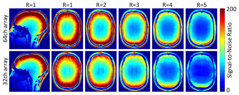
Measured SNR in non-accelerated (R = 1) and one-dimensional accelerated (R = 3 to R = 5) cases for the 64-channel coil (top row) 32-channel coil (bottom row) in a transversal midbrain slice. The 64-channel coil increasingly outperforms the 32-channel coil with higher acceleration factors in both central and peripheral SNR. The scans were accelerated in anterior–posterior direction.

Figure 5.

Relative SNR gain of a 64-channel array coil over a size matched 32-channel coil as a function of acceleration. The higher peripheral SNR of the 64-channel coil and the reduced g-factors, mainly obtained in the center of the 64-channel coil, show substantial better SNR performance in all brain areas with higher accelerated acquisitions compared to the 32-channel array coil.

Figure 6.

Impact of coil overlap on SNR performance in an 4-fold accelerated parallel imaging case on tiles spherical geometry. The numbers in brackets indicate the SNR in the center (left) and the overall image SNR (right) as percentages relative to the case of an 8-channel coil using a touching geometry (red brackets numbers). Large arrays appear to generally favor coil overlap, both for conventional and parallel imaging. (Image courtesy F. Wiesinger, ETH Zuerich; now at GE Global Research, Munich).

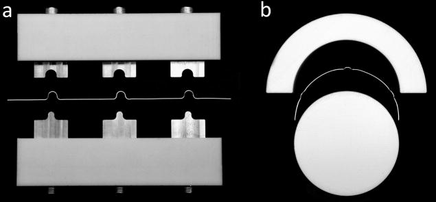
In practice, array geometries tend to use overlaps in at least one direction (to keep the couplings manageable.) Figure 7 shows a simulation comparison between two popular types of brain array layouts [41,44–46] on the same geometrical head former. The arrays modeled in this way are similar to (but not identical too) the commercial cases. The electromagnetic fields were modeled using a full-wave FDTD simulation. The simulation included a conductive load using a human-meshed model (Duke, Virtual Family, with 1mm isotropic resolution) [47]. The overlapped coil showed a higher SNR for non-accelerated imaging in a central ROI as well as higher head-average SNR. But the gapped array shows improved SNR in a ring ROI at the periphery of the brain, consistent with its smaller loop diameters. For accelerated images the gapped array had slightly improved central and overall brain-average g-factor compared to the overlapped array. Putting these two factors together to form the SNR of the accelerated image, the overlapped array outperformed the gapped array for R= 1 to 3, for R=4 the two arrays were nearly identical and for R>5 the gapped array had higher SNR in the accelerated image metric.

Figure 7.

Simulation geometries for time-domain finite element computations for two popular 32-channel brain coil (overlap and partially overlap-gap design). The numbers in brackets indicate the SNR in the center (left) and the overall image SNR (right) as percentages relative to the 32-channel overlapped design without acceleration (red brackets numbers). SNR simulation of a transverse mid-brain slice show higher SNR for non and moderate acceleration cases for the overlapped array geometry, while for higher acceleration factors (R>4), the gapped array better performs.

The ingredients to building a highly parallel array

The basic detection unit of a receiver coil array can be constructed out of any one of a variety of different conductive resonant structures, such as striplines [3,4,48–51], or transverse electromagnetic coils [52], or even from encircled coupled structures such as birdcages [53–55]. However, the most common MR detectors in large N_ch coil arrays are loops. The use of this basic configuration of an LC tuned circuit dates back to Bloch’s original experiment in that a loop coil can be viewed as a single-turn solenoid. The earliest in vivo MR applications of the loop coil used as a surface coil was in the ‘70s [56]. By 1980 the loop surface coil was valued for both its high sensitivity and its ability to spatially localize signal [57].

The loop coil forms a magnetic dipole reception pattern, which couples primarily to magnetic fields in the near-field region. Namely, the alternating external flux produced by the spins induces an EMF in the loop through Faraday’s law. An isolated coil element has resistive losses from its conducting wires, solder joints, losses in the dielectric material of the capacitors and eddy-current losses in any surrounding structures. For a coil near a conductive sample the losses arising from induced eddy currents (from dB/dt) and displacement currents in the sample volume typically dominate all other losses. The fraction of losses dissipated in the body relative to the components is easily measured by comparing the unload Quality factor (Q) of the coil to the loaded Q. Since Q = L/R for an LCR circuit, it is easy to show that R_body/R_comp= Q_UL/Q_L−1. Since body noise is detected through the same mechanism and at the same frequency as the MR signal (Faraday detection at the Larmor frequency), the two cannot be distinguished and efforts to improve the signal detection will necessarily increase the noise level. In this respect, maximum body noise means maximum MR signal with the added benefit that other loss (and therefore noise) sources become negligible. For example, if a Q_UL/Q_L = 6 is achieved, then component losses are 5 fold smaller than the body losses and eliminating them completely will improve the image SNR by less than 10%. If Q_UL/Q_L = 10, elimination of the component losses (e.g. through super conductors etc) improves SNR by a factor of 1.005. This gives the coil engineer a clear picture of when s/he can stop worrying about component losses. The eddy currents and capacitive coupling to the body also produce shifts in resonance frequency upon loading. The principal method for controlling the resonance shifts is to distribute the capacitors around the loop, using multiple large capacitors rather than a single small one.

During RF excitation, assumed to be provided by a uniform body transmit coil, the receiver coil must be detuned to reduce the power transmitted into the Rx chain during Tx. In addition to potentially damaging sensitive electronic components, large currents induced in the Rx coil could also create SAR hotspots of their own and cause heating and injury. Thus, the receiver coil must be “transparent”, i.e., it must not distort the B₁⁺ profile of the volume excitation coil during Tx. This can be achieved by limiting the induced currents to negligible levels by switching on high impedance elements in the coil loop [58,59]. In the most common configuration an detuning trap circuit under active control is incorporated into the loop. This comprises a PIN diode and a series inductor which resonates at the Larmor frequency across one of the capacitors from the loop. The diode acts as a switch connecting the parallel resonant trap to the coil, thus, inserting a high impedance parallel LC circuit in series in the loop. As a redundant safety feature, passive elements are often also employed incase the active system fails. One popular passive device is to bridge a second LC trap with passive crossed diodes [59–61] or to use an RF fuse in the loop. At the output port of the loop coil an impedance transformation network is needed to couple power out of the resonator into the preamplifier. As will be seen in the next section, we do not transform the impedance of the coil with a view toward achieving a power match with the preamplifier (no reflected power), but the less limiting constraint of presenting the preamplifier with the load that minimizes its noise figure. Thus if the input impedance of the preamplifier is Z_{preamp_in}, this does not require the coil element to be transformed to Z_{preamp_in}* which is the “power match” which eliminates reflected power, but to Z_{noise_fig_opt}, which can be considerably different.

While MR coil engineers typically prefer to work with arrays with little or no mutual coupling, there is some evidence that modest decoupling is relatively unimportant if the image is combined with either the cov-rSoS or optimal-SNR method [62]. These methods already utilize the noise covariance matrix, as do accelerated image reconstruction methods like SENSE which also utilizes coil sensitivity maps that would describe the coupling [52]. The greatest fear of the beginning coil builder is that the coupling will perturb the resonance frequency of the carefully tuned high-Q resonators rendering them insensitive to the Larmor frequency. We show below that this fear is ungrounded when preamplifier decoupling is used. Nevertheless, coupling between multiple elements makes it difficult to transform the impedance of the element to Z_{noise_fig_opt}. In addition, noise in the preamplifier can project back into the coil and then couple to other elements. This added noise appears on the diagonals of the noise covariance matrix and is therefore not mitigated with inclusion of the matrix [63,64]. Finally we note that at some point, if all the elements are coupled enough to give identical profiles, parallel MRI reconstructions will become highly ill-conditioned; i.e. the sensitivity patterns contain less distinct spatial information than the uncoupled coils would.

Several strategies have been proposed for removing the effects of mutual inductance. First, the overlap of adjacent coil elements may be carefully adjusted to the “critical overlap” so that the shared flux between adjacent coils is zero [65,66]. For circular loops in a plane, the critical overlap is achieved with a distance between centers of 0.75 times the diameter. While convenient, this strategy restricts the geometrical layouts of the coil elements; only certain repeating symmetry patterns can be used to tile a given geometry. For example, the critical overlap allows a hexagonal tiling pattern of 6 loops surrounding 1 to tile a plane or cylinder with all nearest neighbors decoupled or a soccer ball (“buckyball”) type pattern of hexagons and pentagons (one pentagon surrounded by 5 hexagons) for a sphere. Alternatively, capacitive or inductive connections or even networks may be built between coils that can exactly cancel the mutual inductance between them [67–69].

Preamplifier decoupling, as described by Roemer and colleagues [8] has become one of the most important tools in constructing large arrays. It deftly exploits a degree of freedom created when the array is receive-only. Namely, the coil element does not need to be power matched to the input impedance of the preamplifier. Instead, the element needs to present a load that minimizes the preamplifier’s noise-figure; a condition that can be different from the power match condition. This frees the coil tuner from being a slave to 50 Ohm systems and coupling power out of the resonator using critical-coupling. Prior to Roemer, practitioners would construct an impedance transformation circuit (at its simplest a capacitor voltage divider) that would transform the small residual resistance in the LC circuit to 50 Ohms. For example, in Fig. 8a the capacitors C₁ and C₂ are chosen to transform the impedance of the resonant loop, r, to present a 50 Ohm impedance to the preamplifier, which itself has a 50 Ohm input impedance. The preamplifier should be designed to have a minimum noise figure when loaded with 50 Ohms. A 50 Ohm transmission line (not shown in Fig. 8) could bring the power coupled out of the resonator to the preamplifier. The power matching condition insures critical-coupling. In this case half the energy stored in the resonator is removed every cycle and the Q of the system is decreased by a factor of 2 when the preamplifier is added. The impedance matching ensures no reflected wave returns power back into the coil. Because Q is only lowered by a factor of 2, the Q involved is still relatively high, and a perturbation that shifts the resonance of the coil off the Larmor frequency could be catastrophic. For example, if the coil loop is bent the inductance and thus resonant frequency is shifted, or if a neighbor inductively couples with it a split-resonance is formed. In these cases, the resonance frequency can be shifted by its half-width or more, reducing the detection efficiency by 2x or more.

Figure 8.

Preamplifier schematics for array imaging. a) shows the standard non-array strategy where the coil is tuned and matched to 50 Ohms and connected to a preamplifier with a 50Ohm input impedance and a 50 Ohm noise match. b) shows an idealized configuration where a high impedance preamplifier is inserted in the tuned loop. For optimal performance this preamplifier would have optimal noise figure with the low-impedance (r) load presented by the loaded coil on resonance. c) shows the standard configuration for array coils. The coil is tuned to the Larmor frequency and matched by C₁ and C₂ to present the desired load which minimizes the preamps noise figure (noise match). The low impedance of the preamplifier (typically 1–2 Ohms) essentially short-circuits the inductor L across C₂. Since L and C₂ are tuned to resonate at the Larmor frequency, this forms a high impedance in series in the loop. The result is effectively equivalent to (b).

The preamplifier decoupling scheme protects us from these scenarios. It does not directly reduce the mutual inductance (like the critical overlap method). Instead, it alters how the measurement of the electromotive force (emf) induced by the spins is made, choosing a measurement strategy that naturally suppresses the effects of mutual inductance. The two most basic types of electrical measurements are either a voltage measurement or a current measurement. In the former, a high impedance is inserted in the circuit containing the electromotive force and the voltage across this impedance is measured. Alternatively, a current measurement can be used whereby a galvanometer with low impedance is inserted into the circuit loop containing the emf and the current is measured. Power, of course, is the product of V and I, and choosing an impedance (such as 50 Ohms) for the measurement, basically determines the mixture between these two extremes of measurement (voltage or current). For example choosing 50 Ohms guarantees the ratio; V/I = 50 for any given power. In the preamplifier decoupling strategy, we do not blindly accept a 50 Ohm impedance but make this choice with a view to its effect on coupling. In analogy, a power plant producing a given amount of power P = VI can choose to step up or step down its voltage to transmit it to the city with either a high voltage and low current or vice-versa. The power engineer takes advantage of this degree of freedom to choose high voltage (low current) transmission lines, because Ohmic losses (given by I²R) are the foremost fear. For highly parallel array builders, inductive coupling is the foremost fear. This suggests a voltage measurement (placing a high impedance in the coil loop) should be chosen, since the reduced current also reduces the effect of inductive coupling.

Thus, instead of choosing the some-what arbitrary 50 Ohm matching condition, the preamplifier/coil circuit is designed so that the preamplifier performs a voltage measurement across the loop. Thus the output circuitry (e.g. match + coax + preamplifier) forms a series high impedance in the tuned loop reducing current flow and thus reducing inductive coupling with other loop elements. Figure 8b shows the desired configuration. Here a high input impedance preamplifier is used and L and C₁₂ are chosen to resonate leaving only real impedances in the loop at the Larmor frequency. For this to work well, the high impedance preamplifier would need a good noise figure when loaded with the low impedance load (r at the Larmor frequency). It is more practical to construct a preamplifier that has a very low input impedance and a noise match of around 50 Ohms. In this case, the circuit in Figure 8c provides the needed transformations. Working back from the preamplifier, the 1Ω input impedance creates a near short connecting the inductor L₁ across C₂. If these two components are chosen to resonant at the Larmor frequency, they form a parallel LC circuit in series in the loop. A very low loss LC parallel circuit has a high impedance on resonance. Thus for the Larmor frequency signals of interest, this configuration places a high impedance in series in the loop reducing the currents induced by neighboring loops and reducing the effective inductive coupling. Working forward from the coil, the capacitors C₁ and C₂ are chosen so that together with L₁, the coil’s impedance is transformed to a value which minimizes the preamplifer noise figure. Typically the preamplifier is still constructed to have minimum noise for a 50 Ohm load, but sometimes a higher impedance is used.

The preamplifier decoupling circuit changes how we look at the basic coil element in ways that effect how highly parallel array coils are constructed. For example, the measurement can now be viewed as a pseudo-wideband device since it “spoils” the Q of the circuit. As mentioned, if a traditional high-Q loop critically coupled into a preamp is mis-tuned, it quickly loses its ability to detect signals. For a Q of 100, at a Larmor frequency of 125MHz, a shift of 1.25MHz shifts the operating point 3dB down from the peak response, losing half the signal. Sadly, the ionic noise currents are present at all frequencies, and thus their power is not diminished. In the preamplifier decoupling case, a mis-tuning of the coil has very little effect on the signal level, thanks to the high impedance nature of the measurement. If the coil is detuned by a few MHz, almost no loss of SNR is detected. It is very informative to try this experiment either on the bench using a rigidly placed loop probe as a “signal source” and the output of the preamplifier routed into the other port of a vector network analyzer setup for S₁₂ measurement. Place the cursor at the Larmor frequency and adjust a trimming capacitor in the loop. The power output at the Larmor frequency does not change. Note that if the coil tuning is changed too much, other effects crop up. For example, if the loop is mis-tuned by more than a few MHz, then its impedance is changed enough so that the preamplifier no longer feels the proper load for minimum noise figure and the image SNR will degrade. Also note that the measurement is not truly broad-band. The preamplifier decoupling itself is highly frequency dependent, and if the Larmor frequency is changed, the whole system falls apart. But the tuning of the loop coil itself is not of critical importance. Thus, in the highly parallel array, we strive firstly to obtain a high- quality preamplifier decoupling using high Q components for C₂, L₁ which are carefully tuned to be on-resonance at the Larmor frequency and to choose very low input impedance preamplifiers. The second most important tuning step is to adjust the C₁ to C₂ ratio (and L₁) so that the preamplifier noise figure is minimum when the coil is loaded on the body. The loop itself must be tuned within a few MHz of the Larmor frequency, but it can actually be advantageous to have a distribution of center-frequencies present, as further reduces inductive coupling [70].

Steps in building and decoupling a large array

The high degree of parallelism requires systemized design, construction and testing in order to implement the large number of tuned receive circuits and optimize their mutual interactions. This has altered the workflow for how we construct receive arrays. The plan for even the final steps, such as the placement of the preamps and the routing of their outputs to the coil plugs, needs to be in place from the beginning. The final bench-tests need to be under conditions similar to those in the scanner bore requiring a coil interface simulator and body-shaped loading phantom. We find that little is gained by testing individual elements separated from the array; the troublesome effects come from neighboring elements and output wiring.

The first step is the design of the close-fitting coil former. A well-implemented design for the former constitutes half the battle. Digital 3D meshing programs allow body shapes to be brought into a CAD program, allowing the physical layout of the array to be performed with precise knowledge of the location of the elements relative to the anatomy of interest (Figs. 9a). The tiling pattern can be laid out on the former, guiding construction (Figs. 9b). After the location of the loops is marked, the locations for the preamplifier connections are decided. Preamps must be orientated in z-direction to minimize Hall effect issues [71–73]. Furthermore the output cable routing must be planned so that these coaxes do not pass near another preamplifier’s input in order to eliminate oscillations. If an output cable length exceeds about 1/8 of the wavelength, a cable trap must be used to eliminate common-mode currents induced by the body RF transmit. Similarly bias lines for the PIN diode detuning must be broken up with either chokes or traps. Ideally, the stands for each preamp and cable trap are integrated into the former model and fabricated as a single unit (e.g. using 3D printing, which is now readily available through online services.)

Figure 9.

Steps in array coil design and construction of a 64-channel head-neck coil array. The helmet shape is taken by dilating the 95th percentile contour of aligned 3D MRI scans (a). Given the geometrical constraints of the split-able anatomical shaped former and knowledge of the anatomical coverage, loop pattern (hexagons/pentagons) can be laid out (b) and engraved directly onto the helmet (c). Loop conductors are cut, bent and assembled over the whole array (d). After preamplifier placing and cabling, the coil is ready for tuning, matching, and decoupling procedures (e).

The geometry and material of the conductors for the loop elements can have a large effect on the highly parallel array. To first approximation, the lowest loss conductors are desired so that body losses significantly out weigh component losses. Kumar and colleagues have attributed an effective noise figure to each component and analyzed the tradeoffs of introducing more series capacitors to the loop [74]. They also noted that while the largest copper trace widths have the lowest loss in a single isolated loop, this was not necessarily best for the array. Namely, a given loop experiences losses in its own conductors and eddy current losses in the surrounding copper. This second, typically overlooked mechanism, meant that using thinner traces, or small diameter wire can be a better strategy for the array. This observation has also been empirically born out when testing a 96 channel brain array [39]. Although it would seem that using wire over printed circuit-board would constitute a fabrication nightmare, we find its relatively easy to stamp out curved wire loop-sections (Fig. 10), including pre-bended the needed bridges to allow one conductor to pass under the other.

Figure 10.

Loop conductor fabrication. Bridges are bend into the loop wire to allow the coil conductors to crossover one another without touching (a). Wires are pre-formed to semicircles with the needed diameter (b).

Early in the process, test loops are constructed (Fig. 11b) to determine the values of the needed components for tuning, matching, preamplifier decoupling, and active and passive detuning traps. The critical overlap ratio of a pair of loops should be checked to guide the layout. After the loop component values are known, we build up the array on the former. We find it impractical to mass-produce elements and then mount them on the former. Better is to build up the elements on the former, checking the active and preamp detuning, tuning, matching and nearest neighbor decoupling as we go. But some components can be mass-produced. For example the circuit board containing the output and active detuning circuitry can be assembled and the PIN diode trap be tuned. Similarly the circuit board section for the tuning capacitors can be pre-constructed and placed on the former. Next, the loop conductors (e.g. copper wire, or circuit board traces) are cut, bent and assembled over the whole array (Fig 9c, Fig. 10, and Fig. 11d). Then, the preamplifier mounting boards are attached and the bias tee circuitry for the PIN diode detuning is wired to the coil plugs (Fig. 9e and Fig 11e). This allows complete control of the active detuning by the coil interface simulator while the coil is being tuned on the bench.

Figure 11.

Some captured details of coil array construction. Starting with a well-designed helmet (a), constructed test loops (b) deliver the needed component values for all next array elements. After assembling the array (c), it is time for carefully adjusting the detuning traps of each element in order to isolate loops under test for proper tuning, matching, decoupling etc. Then, preamplifier boards are attached and the bias tee circuitry for the PIN diode detuning is wired to the coil plugs (e). Using a coil plug simulator, loops can be individually controlled and adjusted. After a detuning check of all elements, neighboring coils are adjusted for critical overlap (f), followed by fine-tuning/matching and preamp decoupling.

Since the first test loops should have provided us with a good guess of the critical overlap ratio and capacitor values, the loops should be near their proper tune and match as well as decoupling. At this stage, however, its best to go through each loop with all other loops actively detuned by their PIN diode traps, checking the active detuning of each loop through and S₂₁ measurement between two inductive probes lightly coupled to the coil loop (achieving >35dB difference between these states). Then the same S₂₁ probe is used to tune of each loop (with all other loops detuned). Next we replace the preamplifier with a dummy preamp board to allow a direct S11 measurement of the load seen by the preamp. Using two such connections, we reduce inductive coupling by measuring S₂₁ between coil pairs (with all other loops detuned) and adjusting the overlap while watching S₂₁ (Fig 9f). For wires loops, the final critical overlap can be easily adjusted by slightly bending the wire (or just manually bending the crossing bridges on the loops). After this adjustment, the impedance of the loop is often altered. The same test set-up is used to readjust to the desired 50 Ohm noise-match.

This optimization of all next neighbors is one of the most time consuming adjustment procedure during phased array construction. After completing all combinations of elements, a second decoupling go-thru is highly recommended. After this step, the array coil should look and functioning like a proper decoupled array and is ready for a final bench touch up. Here we re-test the active detuning and preamplifier decoupling. This is done with the array plugged into the simulator (controlling PIN diode biases and supplying DC power to each preamp). The active detuning and preamplifier decoupling are checked and when needed the coil matching or cable length is adjusted so that the “preamp dip” is exactly at the Larmor frequency on the S₂₁ measurement of the loop in the receive state and the active detuning achieves >35dB detuning. Either the two loosely coupled probes can be used for this final S₂₁ measurement, or better still, a single probe connected to the attenuated output port of the network analyzer and held near the loop. The output of the powered preamplifier is connected to the detector port of the network analyzer and S12 is measured. Finally the cable traps are checked with an S₁₂ current injection probe measurement.

Experience with massively parallel arrays

The early success with 16, 24 and 32-channel brain arrays [17,44,46,48,49,75–81] has lead to commercial 32-channel brain arrays and experimentation with 64, 90 and 96-channel brain arrays [39,41,82,83]. Similarly, cardiac/chest coils with 32 elements have been established in experimental settings [76,84–89] and have been followed up with 128-channel arrays [90,91]. Several highly parallel detectors have been constructed for ¹²⁹Xe and ³He hyperpolarized gases where the acceleration capability is important for efficiently utilizing the polarization [92–95]. Increased reliance on the array as a primary device for image encoding, will likely lead to considerably higher numbers of detectors than would be contemplated from sensitivity arguments alone. In this scenario, the role of the MR detector array begins to more resemble the electroencephalography (EEG) or magnetoencephalography (MEG) detector, where all of the spatial information is derived from the detector geometry. While we continue to think of the gradient coil as the principal “encoder” of the MR image, that view is becoming outdated. With acceleration in two directions, acceleration factors of above 10 fold can be achieved. Thus, the gradients account for as little as 10% of the encoding; the rest of the burden being placed on the receive array. While the “ultimate” g-factor theory tells us there are limits to the ability of arrays to encode, primarily from the fundamental smoothness of solutions to Maxwell’s equations as you penetrate deeply into the object [34,35,37], planar 64-channel arrays in the very near field show that there is virtually no limit to using the spatial information of the arrays to encode [96–98]. Figure 12 shows a high resolution (1mm × 1mm × 2mm) spin echo EPI brain image acquired with a 96-channel array at accelerations of R=4,5,6, and 8×, demonstrating the ability of the array to achieve its expected acceleration in one dimension (R~6), which is relatively near the expected limit of 1-D acceleration. Figure 13 shows the benefit of acceleration for clinical imaging, where the sensitivity and acceleration gains of a 64-channel brain array are used for detailed, high-resolution, T1 and T2 full brain anatomical imaging at reasonable scan times (Fig. 13a/b: MPRAGE, 3.38 min, 1mm iso; Fig. 13c/d: T2-SPACE, 2.19 min, 0.47×0.47×0.6mm³). Figure 14 shows the benefit of accelerating via simultaneously acquired slices for functional brain imaging. Here the acquisition speed is accelerated 10-fold by exciting and simultaneously reading out 10 slices, and then the aliased images are unaliased with the array information [99–101]. In this case, no k-space lines are left out so there is no (10) penalty; only a g-factor penalty. This method has essentially removed the temporal sampling barrier from functional MRI [102]. Finally, Fig. 15 shows an extreme example of accelerating the encoding in each of 2 spatial directions. Here, Mansfield’s original proposal [103] of fully encoding the 3D head after a single excitation is realized due to the acquisition of only 1/20^th of the phase encoding lines. This allowed 3.4mm resolution whole brain acquisitions as fast as 10 frames per second [104,105].

Figure 12.

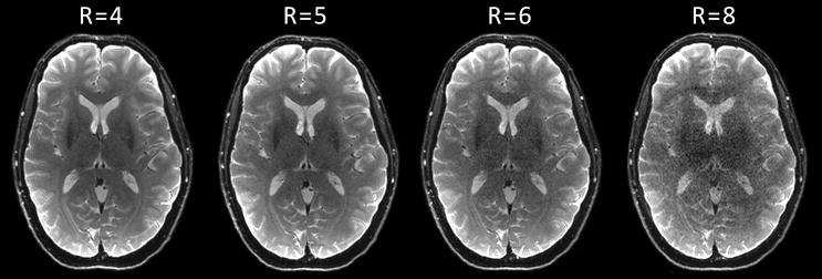
High resolution single-shot gradient-echo EPI images with GRAPPA acceleration factors from R=3 to R=8 in anterior-posterior direction, obtained with the 96-channel coil array.

Figure 13.

Fully encoded highly accelerated anatomical brain images. Top row: transversal (a) and sagittal (b) 1mm isotropic MPRAGE images with GRAPPA acceleration factor of R = 4 and an acquisition time of 3:38 minutes for whole head coverage. Bottom row: sagittal T2-SPACE images with highly 2D-GRAPPA acceleration of R=6 (R=3 in-plane and R=2 through-plane) and an in-plane resolution of 0.47×0.47mm², and 0.9 mm slice thickness. Acquisition time was 2:19 minutes for whole head coverage

Figure 14.

Whole brain EPI images acquired with 10 slices accelerated simultaneously and then unaliased using the 64-channel brain array’s spatial information. This “simultaneous multi-slice” or “multi-band” method allows the temporal resolution of the fMRI acquisition to be increased, in this case by an order of magnitude allowing the 60 slices needed to cover the brain for this 2mm isotropic resolution image set to be obtained in about 0.5s. (Image courtesy of K. Setsompop, MGH).

Figure 15.

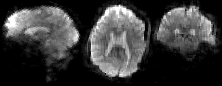
Whole-brain single-shot 3T Echo Volume Image (EVI). The whole brain image is encoded in a single shot in less a 77.3 ms echo-volume trajectory allowing a temporal resolution of 120ms. Image volume reformatted in axial, coronal and sagittal planes. The matrix was 64×64×56 using a 24cm FOV, resulting in 3.4 mm nominal spatial resolution. The fully encoded 64×56 = 3584 lines of k-space was curtailed by a factor 16x acceleration (4x in each of the two phase encode directions), and by the 6/8 partial Fourier acquisition yielding a readout of 168 lines with a 77.3 ms duration. The effective echo-spacing in the slowest phase encode direction was 1.38 ms resulting in relatively high distortions compared to 2D EPI. (Image courtesy of T. Witzel, MGH).

Conclusions

With 32-channel array coils now widely available, massively parallel array detection appears to be the future for high sensitively, rapidly acquired clinical and research MR imaging. They have changed the way we think about MR detection; for example by extending our SNR analysis to correctly account for the channel combination effects and the need to consider both accelerated and non-accelerated imaging SNR. They have also caused a deviation from the standard way of thinking about the receive element as a resonator with critical coupling transferring power to the preamplifier without reflections. Practical experience shows that the biggest barrier to going beyond 128 channels is the ability to keep the ever-smaller array elements body-load dominated. Higher fields, flexible formers and perhaps cooled components will aid here. Analysis of the ceiling imposed by Maxwell’s equations shows that paradoxically, the center of the body is the easiest location for arrays to fulfill their theoretical potential. Nonetheless these analyses show that at the periphery of the body we still have significant progress to be made, especially at 7T and for highly accelerated acquisitions. The synergy between field strength and highly parallel detection and accelerated imaging will likely ensure that these two methods will continue to evolve together in a productive way. Realization of the potential of massively parallel arrays is in its infancy, but has already shown its potential in improving clinical imaging and enabling encoding-limited applications.

Highlights.

• We show the theoretical and experimental basis for the trend towards higher channel counts.

• We show how to optimally combine array data for maximum signal-to-noise ratio.

• The ingredients to building a highly parallel array.

• Needed changes in radio-frequency methodology for constructing massively arrays.

• Examples of state-of-the-art for highly accelerated imaging with highly parallel arrays.

References

- 1.Leussler C, Stimma J, Roschmann P. The bandpass birdcage resonator modified as a coil array for simultaneous MR acquisition. Proceedings of the 5th Annual Meeting of ISMRM; Vancouver. 1997. p. 176. [Google Scholar]
- 2.Katscher U, Börnert P, Leussler C, van den Brink JS. Transmit SENSE. Magn Reson Med. 2003;49:144–150. doi: 10.1002/mrm.10353. [DOI] [PubMed] [Google Scholar]
- 3.Adriany G, Van de Moortele P-F, Wiesinger F, Andersen P, Strupp JP, Zhang X, Snyder CJ, Chen W, Pruessmann KP, Boesiger P, Vaughan T, Ugurbil K. Transceive Stripline Arrays for Ultra High Field Parallel Imaging Applications. Proceedings of the 11th Annual Meeting of ISMRM; Toronto. 2003. p. 474. [Google Scholar]
- 4.Adriany G, Van de Moortele P-F, Wiesinger F, Moeller S, Strupp JP, Andersen P, Snyder C, Zhang X, Chen W, Pruessmann KP, Boesiger P, Vaughan T, Uğurbil K. Transmit and receive transmission line arrays for 7 Tesla parallel imaging. Magn Reson Med. 2005;53:434–445. doi: 10.1002/mrm.20321. [DOI] [PubMed] [Google Scholar]
- 5.Fontius U, Baumgartl R, Boettcher U, Doerfler G, Hebrank F, Fischer D, Jeschke H, Kannengiesser SAR, Kwapil G, Nerreter U, Nistler J, Pirkl G, Potthast A, Roell S, Schor S, Stoeckel B, Adelsteinson E, Adriany G, Alagappan V, Gagoski BA, Setsompop K, Wald LL, Schmitt F. A flexible 8-channel RF transmit array system for parallel excitation. Proceedings of the 14th Annual Meeting of ISMRM; Seattle. 2006. p. 127. [Google Scholar]
- 6.Greasslin I, Vernickel P, Schmidt J, Findeklee C, Röschmann P, Leussler C, Haaker P, Laudan H, Luedeke KM, Scholz J, Buller S, Keupp J, Börnert P, Dingemans H, Mens G, Vissers G, Blom K, Swennen N, vd Heijden J, Mollevanger L, Harvey P, Katscher U. Whole Body 3T MRI System with Eight Parallel RF Transmission Channels. Proceedings of the 14th Annual Meeting of ISMRM; Seattle. 2006. p. 129. [Google Scholar]
- 7.Alagappan V, Nistler J, Adalsteinsson E, Setsompop K, Fontius U, Zelinski A, Vester M, Wiggins GC, Hebrank F, Renz W, Schmitt F, Wald LL. Degenerate mode band-pass birdcage coil for accelerated parallel excitation. Magn Reson Med. 2007;57:1148–1158. doi: 10.1002/mrm.21247. [DOI] [PubMed] [Google Scholar]
- 8.Roemer PB, Edelstein WA, Hayes CE, Souza SP, Mueller OM. The NMR phased array. Magn Reson Med. 1990;16:192–225. doi: 10.1002/mrm.1910160203. [DOI] [PubMed] [Google Scholar]
- 9.Hayes CE, Hattes N, Roemer PB. Volume imaging with MR phased arrays. Magn Reson Med. 1991;18:309–319. doi: 10.1002/mrm.1910180206. [DOI] [PubMed] [Google Scholar]
- 10.Constantinides CD, Westgate CR, O’Dell WG, Zerhouni EA, McVeigh ER. A phased array coil for human cardiac imaging. Magn Reson Med. 1995;34:92–98. doi: 10.1002/mrm.1910340114. [DOI] [PMC free article] [PubMed] [Google Scholar]
- 11.Foo TK, MacFall JR, Sostman HD, Hayes CE. Single-breath-hold venous or arterial flow-suppressed pulmonary vascular MR imaging with phased-array coils. J Magn Reson Imaging. 1993;3:611–616. doi: 10.1002/jmri.1880030410. [DOI] [PubMed] [Google Scholar]
- 12.Hayes CE, Dietz MJ, King BF, Ehman RL. Pelvic imaging with phased-array coils: quantitative assessment of signal-to-noise ratio improvement. J Magn Reson Imaging. 1992;2:321–326. doi: 10.1002/jmri.1880020312. [DOI] [PubMed] [Google Scholar]
- 13.Hayes CE, Mathis CM, Yuan C. Surface coil phased arrays for high-resolution imaging of the carotid arteries. J Magn Reson Imaging. 1996;6:109–112. doi: 10.1002/jmri.1880060121. [DOI] [PubMed] [Google Scholar]
- 14.Hardy CJ, Bottomley PA, Rohling KW, Roemer PB. An NMR phased array for human cardiac 31P spectroscopy. Magn Reson Med. 1992;28:54–64. doi: 10.1002/mrm.1910280106. [DOI] [PubMed] [Google Scholar]
- 15.Wald LL, Moyher SE, Day MR, Nelson SJ, Vigneron DB. Proton spectroscopic imaging of the human brain using phased array detectors. Magn Reson Med. 1995;34:440–445. doi: 10.1002/mrm.1910340322. [DOI] [PubMed] [Google Scholar]
- 16.Hayes CE, Tsuruda JS, Mathis CM. Temporal lobes: surface MR coil phased-array imaging. Radiology. 1993;189:918–920. doi: 10.1148/radiology.189.3.8234726. [DOI] [PubMed] [Google Scholar]
- 17.Porter JR, Wright SM, Reykowski A. A 16-element phased-array head coil. Magn Reson Med. 1998;40:272–279. doi: 10.1002/mrm.1910400213. [DOI] [PubMed] [Google Scholar]
- 18.Wald LL, Carvajal L, Moyher SE, Nelson SJ, Grant PE, Barkovich AJ, Vigneron DB. Phased-array detectors and an automated intensity-correction algorithm for high-resolution MR imaging of the human brain. Magn Reson Med. 1995;34:433–439. doi: 10.1002/mrm.1910340321. [DOI] [PubMed] [Google Scholar]
- 19.Carlson JW. An algorithm for NMR imaging reconstruction based on multiple RF receiver coils. J Magn Reson. 1987;74:376–380. [Google Scholar]
- 20.Hutchinson M, Raff U. Fast MRI data acquisition using multiple detectors. Magn Reson Med. 1988;6:87–91. doi: 10.1002/mrm.1910060110. [DOI] [PubMed] [Google Scholar]
- 21.Kelton JR, Magin RL, Wright SM. An algorithm for rapid image acquisition using multiple receiver coils. Proceedings of the 8th Annual Meeting of SMRM; Amsterdam. 1989. p. 1172. [Google Scholar]
- 22.Kwiat D, Einav S, Navon G. A decoupled coil detector array for fast image acquisition in magnetic resonance imaging. Med Phys. 1991;18:251–265. doi: 10.1118/1.596723. [DOI] [PubMed] [Google Scholar]
- 23.Ra JB, Rim CY. Fast imaging using subencoding data sets from multiple detectors. Magn Reson Med. 1993;30:142–145. doi: 10.1002/mrm.1910300123. [DOI] [PubMed] [Google Scholar]
- 24.Sodickson DK, Manning WJ. Simultaneous acquisition of spatial harmonics (SMASH): fast imaging with radiofrequency coil arrays. Magn Reson Med. 1997;38:591–603. doi: 10.1002/mrm.1910380414. [DOI] [PubMed] [Google Scholar]
- 25.Pruessmann KP, Weiger M, Scheidegger MB, Boesiger P. SENSE: sensitivity encoding for fast MRI. Magn Reson Med. 1999;42:952–962. [PubMed] [Google Scholar]
- 26.Gudbjartsson H, Patz S. The Rician distribution of noisy MRI data. Magn Reson Med. 1995;34:910–914. doi: 10.1002/mrm.1910340618. [DOI] [PMC free article] [PubMed] [Google Scholar]
- 27.Kellman P, McVeigh ER. Image reconstruction in SNR units: a general method for SNR measurement. Magn Reson Med. 2005;54:1439–1447. doi: 10.1002/mrm.20713. [DOI] [PMC free article] [PubMed] [Google Scholar]
- 28.Henkelman RM. Measurement of signal intensities in the presence of noise in MR images. Med Phys. 1985;12:232–233. doi: 10.1118/1.595711. [DOI] [PubMed] [Google Scholar]
- 29.Lenglet C, Sotiropoulos S, Moeller S, Xu J, Auerbach EJ, Yacoub E, Feinberg D, Setsompop K, Wald LL, Behrens TE, Ugurbil K. Multichannel Diffusion MR Image Reconstruction: How to Reduce Elevated Noise Floor and Improve Fiber Orientation Estimation. Proceedings of the 20th Annual Meeting of ISMRM; Melbourne. 2012. p. 3538. [Google Scholar]
- 30.Griswold MA, Jakob PM, Heidemann RM, Nittka M, Jellus V, Wang J, Kiefer B, Haase A. Generalized autocalibrating partially parallel acquisitions (GRAPPA) Magn Reson Med. 2002;47:1202–1210. doi: 10.1002/mrm.10171. [DOI] [PubMed] [Google Scholar]
- 31.Breuer FA, Kannengiesser SAR, Blaimer M, Seiberlich N, Jakob PM, Griswold MA. General formulation for quantitative G-factor calculation in GRAPPA reconstructions. Magn Reson Med. 2009;62:739–746. doi: 10.1002/mrm.22066. [DOI] [PubMed] [Google Scholar]
- 32.Robson PM, Grant AK, Madhuranthakam AJ, Lattanzi R, Sodickson DK, McKenzie CA. Comprehensive quantification of signal-to-noise ratio and g-factor for image-based and k-space-based parallel imaging reconstructions. Magn Reson Med. 2008;60:895–907. doi: 10.1002/mrm.21728. [DOI] [PMC free article] [PubMed] [Google Scholar]
- 33.Hayes CE, Axel L. Noise performance of surface coils for magnetic resonance imaging at 1.5 T. Med Phys. 1985;12:604–607. doi: 10.1118/1.595682. [DOI] [PubMed] [Google Scholar]
- 34.Wiesinger F, Boesiger P, Pruessmann KP. Electrodynamics and ultimate SNR in parallel MR imaging. Magn Reson Med. 2004;52:376–390. doi: 10.1002/mrm.20183. [DOI] [PubMed] [Google Scholar]
- 35.Wiesinger F, De Zanche N, Pruessmann KP. Approaching ultimate SNR with finite coil arrays. Proceedings of the 13th Annual Meeting of ISMRM; Miami. 2005. p. 672. [Google Scholar]
- 36.Ocali O, Atalar E. Ultimate intrinsic signal-to-noise ratio in MRI. Magn Reson Med. 1998;39:462–473. doi: 10.1002/mrm.1910390317. [DOI] [PubMed] [Google Scholar]
- 37.Ohliger MA, Grant AK, Sodickson DK. Ultimate intrinsic signal-to-noise ratio for parallel MRI: electromagnetic field considerations. Magn Reson Med. 2003;50:1018–1030. doi: 10.1002/mrm.10597. [DOI] [PubMed] [Google Scholar]
- 38.Lattanzi R, Grant AK, Polimeni JR, Ohliger MA, Wiggins GC, Wald LL, Sodickson DK. Performance evaluation of a 32-element head array with respect to the ultimate intrinsic SNR. NMR Biomed. 2010;23:142–151. doi: 10.1002/nbm.1435. [DOI] [PMC free article] [PubMed] [Google Scholar]
- 39.Wiggins GC, Polimeni JR, Potthast A, Schmitt M, Alagappan V, Wald LL. 96-Channel receive-only head coil for 3 Tesla: design optimization and evaluation. Magn Reson Med. 2009;62:754–762. doi: 10.1002/mrm.22028. [DOI] [PMC free article] [PubMed] [Google Scholar]
- 40.Reykowski A. How to calculate the SNR limit of SENSE related reconstruction techniques. Proceedings of the 10th Annual Meeting of ISMRM; Honolulu. 2002. p. 905. [Google Scholar]
- 41.Keil B, Blau JN, Biber S, Hoecht P, Tountcheva V, Setsompop K, Triantafyllou C, Wald LL. A 64-channel 3T array coil for accelerated brain MRI. Magn Reson Med. 2012 doi: 10.1002/mrm.24427. [Epub ahead of print] [DOI] [PMC free article] [PubMed] [Google Scholar]
- 42.Weiger M, Pruessmann KP, Leussler C, Röschmann P, Boesiger P. Specific coil design for SENSE: a six-element cardiac array. Magn Reson Med. 2001;45:495–504. doi: 10.1002/1522-2594(200103)45:3<495::aid-mrm1065>3.0.co;2-v. [DOI] [PubMed] [Google Scholar]
- 43.de Zwart JA, Ledden PJ, Kellman P, van Gelderen P, Duyn JH. Design of a SENSE-optimized high-sensitivity MRI receive coil for brain imaging. Magn Reson Med. 2002;47:1218–1227. doi: 10.1002/mrm.10169. [DOI] [PubMed] [Google Scholar]
- 44.Ledden PJ, Mareyam A, Wang S, van Gelderen P, Duyn J. 32-Channel Receive-Only SENSE Array for Brain Imaging at 7T. Proceedings of the 15th Annual Meeting of ISMRM; Berlin. 2007. p. 242. [Google Scholar]
- 45.Wang S, de Zwart JA, Duyn JH. A fast integral equation method for simulating high-field radio frequency coil arrays in magnetic resonance imaging. Phys Med Biol. 2011;56:2779–2789. doi: 10.1088/0031-9155/56/9/010. [DOI] [PMC free article] [PubMed] [Google Scholar]
- 46.Wiggins GC, Triantafyllou C, Potthast A, Reykowski A, Nittka M, Wald LL. 32-channel 3 Tesla receive-only phased-array head coil with soccer-ball element geometry. Magn Reson Med. 2006;56:216–223. doi: 10.1002/mrm.20925. [DOI] [PubMed] [Google Scholar]
- 47.Christ A, Kainz W, Hahn EG, Honegger K, Zefferer M, Neufeld E, Rascher W, Janka R, Bautz W, Chen J, Kiefer B, Schmitt P, Hollenbach H-P, Shen J, Oberle M, Szczerba D, Kam A, Guag JW, Kuster N. The Virtual Family--development of surface-based anatomical models of two adults and two children for dosimetric simulations. Phys Med Biol. 2010;55:1041–1055. doi: 10.1088/0031-9155/55/2/N01. [DOI] [PubMed] [Google Scholar]
- 48.Adriany G, Van de Moortele P-F, Ritter J, Moeller S, Auerbach EJ, Akgün C, Snyder CJ, Vaughan T, Uğurbil K. A geometrically adjustable 16-channel transmit/receive transmission line array for improved RF efficiency and parallel imaging performance at 7 Tesla. Magn Reson Med. 2008;59:590–597. doi: 10.1002/mrm.21488. [DOI] [PubMed] [Google Scholar]
- 49.Adriany G, Auerbach EJ, Snyder CJ, Gözübüyük A, Moeller S, Ritter J, Van de Moortele P-F, Vaughan T, Uğurbil K. A 32-channel lattice transmission line array for parallel transmit and receive MRI at 7 tesla. Magn Reson Med. 2010;63:1478–1485. doi: 10.1002/mrm.22413. [DOI] [PMC free article] [PubMed] [Google Scholar]
- 50.Driesel W, Mildner T, Möller HE. A microstrip helmet coil for human brain imaging at high magnetic fields. Concepts Magn Reson Part B Magn Reson Eng. 2008;33B:94–108. [Google Scholar]
- 51.Lee RF, Hardy CJ, Sodickson DK, Bottomley PA. Lumped-element planar strip array (LPSA) for parallel MRI. Magn Reson Med. 2004;51:172–183. doi: 10.1002/mrm.10667. [DOI] [PMC free article] [PubMed] [Google Scholar]
- 52.Tropp J, Sodickson DK, Ohliger MA. Feasibilty of a TEM Surface Array for Parallel Imaging. Proceedings of the 10th Annual Meeting of ISMRM; Honolulu. 2002. p. 856. [Google Scholar]
- 53.Carlson JW, Minemura T. Imaging time reduction through multiple receiver coil data acquisition and image reconstruction. Magn Reson Med. 1993;29:681–687. doi: 10.1002/mrm.1910290516. [DOI] [PubMed] [Google Scholar]
- 54.Lin F-H, Kwong KK, Huang I-J, Belliveau JW, Wald LL. Degenerate mode birdcage volume coil for sensitivity-encoded imaging. Magn Reson Med. 2003;50:1107–1111. doi: 10.1002/mrm.10632. [DOI] [PubMed] [Google Scholar]
- 55.Mueller MF, Blaimer M, Breuer F, Lanz T, Webb A, Griswold M, Jakob P. Double spiral array coil design for enhanced 3D parallel MRI at 1.5 Tesla. Concepts Magn Reson Part B Magn Reson Eng. 2009;35B:67–79. [Google Scholar]
- 56.Morse OC, Singer JR. Blood Velocity Measurements in Intact Subjects. Science. 1970;170:440–441. doi: 10.1126/science.170.3956.440. [DOI] [PubMed] [Google Scholar]
- 57.Ackerman JJH, Grove TH, Wong GG, Gadian DG, Radda GK. Mapping of metabolites in whole animals by 31P NMR using surface coils. Nature. 1980;283:167–170. doi: 10.1038/283167a0. [DOI] [PubMed] [Google Scholar]
- 58.Boskamp EB. Improved surface coil imaging in MR: decoupling of the excitation and receiver coils. Radiology. 1985;157:449–452. doi: 10.1148/radiology.157.2.4048454. [DOI] [PubMed] [Google Scholar]
- 59.Edelstein WA, Hardy CJ, Mueller OM. Electronic Decoupling of Surface-Coil Receivers for NMR Imaging and Spectroscopy. J Magn Reson. 1986;67:156–161. [Google Scholar]
- 60.Bendall MR. Portable NMR sample localization method using inhomogeneous RF irradiation coils. Chem Phys Lett. 1983;99:310–315. [Google Scholar]
- 61.Hyde JS, Rilling RJ, Jesmanowicz A. Passive decoupling of surface coils by pole insertion. J Magn Reson. 1990;89:485–495. [Google Scholar]
- 62.Duensing GR, Brooker HR, Fitzsimmons JR. Maximizing Signal-to-Noise Ratio in the Presence of Coil Coupling. J Magn Reson Series B. 1996;111:230–235. doi: 10.1006/jmrb.1996.0088. [DOI] [PubMed] [Google Scholar]
- 63.Findeklee C, Duensing R, Reykowski A. Simulating Array SNR & Effective Noise Figure in Dependance of Noise Coupling. Proceedings of the 11th Annual Meeting of ISMRM; Montreal. 2011. p. 1883. [Google Scholar]
- 64.Findeklee C. Array Noise Matching - Generalization. Proof and Analogy to Power Matching. IEEE Trans Antennas Propag. 2011;59:452–459. [Google Scholar]
- 65.Boskamp EB. A new revolution in surface coil technology: the array surface coil. Proceedings of the 6th Annual Meeting of SMRM; New York. 1987. p. 405. [Google Scholar]
- 66.Hyde JS, Jesmanowicz A, Froncisz W, Kneeland JB, Grist TM, Campagna NF. Parallel image acquisition from noninteracting local coils. J Magn Reson. 1986;70:512–517. [Google Scholar]
- 67.Lee RF, Giaquinto RO, Hardy CJ. Coupling and decoupling theory and its application to the MRI phased array. Magn Reson Med. 2002;48:203–213. doi: 10.1002/mrm.10186. [DOI] [PubMed] [Google Scholar]
- 68.Wang J. A novel method to reduce the signal coupling of surface coils for MRI. Proceedings of the 4th Annual Meeting of ISMRM; New York. 1996. p. 1434. [Google Scholar]
- 69.Wu B, Qu P, Wang C, Yuan J, Shen GX. Interconnecting L/C components for decoupling and its application to low-field open MRI array. Concepts Magn Reson Part B Magn Reson Eng. 2007;31B:116–126. [Google Scholar]
- 70.Keil B, Tountcheva V, Triantafyllou C, Wald LL. Reducing Element Coupling in Array Coils using Off-Tuned Elements. Proceedings of the 19th Annual Meeting of ISMRM; Montreal. 2011. p. 1866. [Google Scholar]
- 71.Possanzini C, Bouteljie M. Influence of magnetic field on preamplifiers using GaAs FET technology. Proceedings of the 16th Annual Meeting of ISMRM; Toronto. 2008. p. 1123. [Google Scholar]
- 72.Hoult DI, Kolansky G. A Magnetic-Field-Tolerant Low-Noise SiGe Pre-amplifier and T/R Switch. Proceedings of the 18th Annual Meeting of ISMRM; Stockholm. 2010. p. 649. [Google Scholar]
- 73.Lagore R, Roberts B, Fallone BG, De Zanche N. Comparison of Three Preamplifier Technologies: Variation of Input Impedance and Noise Figure With B0 Field Strength. Proceedings of the 19th Annual Meeting of ISMRM; Montreal. 2011. p. 1864. [Google Scholar]
- 74.Kumar A, Edelstein WA, Bottomley PA. Noise figure limits for circular loop MR coils. Magn Reson Med. 2009;61:1201–1209. doi: 10.1002/mrm.21948. [DOI] [PMC free article] [PubMed] [Google Scholar]
- 75.Keil B, Triantafyllou C, Hamm M, Wald LL. Design Optimization of a 32-Channel Head Coil at 7T. Proceedings of the 18th Annual Meeting of ISMRM; Stockholm. 2010. p. 1493. [Google Scholar]
- 76.Wiggins GC, Triantafyllou C, Potthast A, Reykowski A, Nittka M, Wald LL. A 32 Channel Receive-only Phased Array Head Coil for 3T with Novel Geodesic Tiling Geometry. Proceedings of the 13th Annual Meeting of ISMRM; Miami. 2005. p. 679. [Google Scholar]
- 77.Wiggins GC, Wiggins CJ, Potthast A, Alagappan V, Kraff O, Reykowski A, Wald LL. A 32 Channel Receive-only Head Coil And Detunable Transmit Birdcage Coil For 7 Tesla Brain Imaging. Proceedings of the 14th Annual Meeting of ISMRM; Seattle. 2006. p. 415. [Google Scholar]
- 78.de Zwart JA, Ledden PJ, van Gelderen P, Bodurka J, Chu R, Duyn JH. Signal-to-noise ratio and parallel imaging performance of a 16-channel receive-only brain coil array at 3.0 Tesla. Magn Reson Med. 2004;51:22–26. doi: 10.1002/mrm.10678. [DOI] [PubMed] [Google Scholar]
- 79.Keil B, Alagappan V, Mareyam A, McNab JA, Fujimoto K, Tountcheva V, Triantafyllou C, Dilks DD, Kanwisher N, Lin W, Grant PE, Wald LL. Size-optimized 32-channel brain arrays for 3 T pediatric imaging. Magn Reson Med. 2011;66:1777–1787. doi: 10.1002/mrm.22961. [DOI] [PMC free article] [PubMed] [Google Scholar]
- 80.Cohen-Adad J, Mareyam A, Keil B, Polimeni JR, Wald LL. 32-channel RF coil optimized for brain and cervical spinal cord at 3 T. Magn Reson Med. 2011;66:1198–1208. doi: 10.1002/mrm.22906. [DOI] [PMC free article] [PubMed] [Google Scholar]
- 81.Ledden PJ, Mareyam A, Wang S, van Gelderen P, Duyn J. Twenty-Four Channel Receive-Only Array for Brain Imaging at 7T. Proceedings of the 14th Annual Meeting of ISMRM; Seattle. 2006. p. 422. [Google Scholar]
- 82.Keil B, Biber S, Rehner R, Tountcheva V, Wohlfarth K, Hoecht P, Hamm M, Meyer H, Fischer HJ, Wald LL. A 64-Channel Array Coil for 3T Head/Neck/C-spine Imaging. Proceedings of the 19th Annual Meeting of ISMRM; Montreal. 2011. p. 160. [Google Scholar]
- 83.Wiggins GC, Potthast A, Triantafyllou C, Lin FH, Wiggins CJ, Wald LL. A 96-channel MRI system with 23- and 90-channel phase array head coils at 1.5 Tesla. Proceedings of the 13th Annual Meeting of ISMRM; Miami. 2005. p. 671. [Google Scholar]
- 84.Zhu Y, Hardy CJ, Sodickson DK, Giaquinto RO, Dumoulin CL, Kenwood G, Niendorf T, Lejay H, McKenzie CA, Ohliger MA, Rofsky NM. Highly parallel volumetric imaging with a 32-element RF coil array. Magn Reson Med. 2004;52:869–877. doi: 10.1002/mrm.20209. [DOI] [PMC free article] [PubMed] [Google Scholar]
- 85.Hardy CJ, Cline HE, Giaquinto RO, Niendorf T, Grant AK, Sodickson DK. 32-element receiver-coil array for cardiac imaging. Magn Reson Med. 2006;55:1142–1149. doi: 10.1002/mrm.20870. [DOI] [PMC free article] [PubMed] [Google Scholar]
- 86.Fujita H, Zheng T, Yang X, Herczak J, Weaver J, Okamoto K, Ishihara T. A 1.5T 32-Channel Cardiac Array Coil for Coronary and Whole Heart MRI. Proceedings of the 16th Annual Meeting of ISMRM; Toronto. 2008. p. 1076. [Google Scholar]
- 87.Spencer D, Akao J, Duensing R, Rimkunas D, Saylor C, Niendorf T, Sodickson DK, Rofsky N. Design of a 32 Channel Cardiac Array for Parallel Imaging. Proceedings of the 13th Annual Meeting of ISMRM; Miami. 2005. p. 911. [Google Scholar]
- 88.Lanz T, Kellman P, Nittka M, Greiser A, Griswold MA. A 32 Channel Cardiac Array Optimized for Parallel Imaging. Proceedings of the 10th Annual Meeting of ISMRM; Seattle. 2006. p. 2578. [Google Scholar]
- 89.Snyder CJ, DelaBarre L, Metzger G, Ugurbil K, Vaughan T. 32-Channel Receive Only Array for Cardiac Imaging at 7T. Proceedings of the 19th Annual Meeting of ISMRM; Montreal. 2011. p. 165. [Google Scholar]
- 90.Schmitt M, Potthast A, Sosnovik DE, Polimeni JR, Wiggins GC, Triantafyllou C, Wald LL. A 128-channel receive-only cardiac coil for highly accelerated cardiac MRI at 3 Tesla. Magn Reson Med. 2008;59:1431–1439. doi: 10.1002/mrm.21598. [DOI] [PMC free article] [PubMed] [Google Scholar]
- 91.Hardy CJ, Giaquinto RO, Piel JE, Rohling KW, Marinelli L, Blezek DJ, Fiveland EW, Darrow RD, Foo TKF. 128-channel body MRI with a flexible high-density receiver-coil array. J Magn Reson Imaging. 2008;28:1219–1225. doi: 10.1002/jmri.21463. [DOI] [PubMed] [Google Scholar]
- 92.Meise FM, Rivoire J, Terekhov M, Wiggins GC, Keil B, Karpuk S, Salhi Z, Wald LL, Schreiber LM. Design and evaluation of a 32-channel phased-array coil for lung imaging with hyperpolarized 3-helium. Magn Reson Med. 2010;63:456–464. doi: 10.1002/mrm.22265. [DOI] [PubMed] [Google Scholar]
- 93.Dregely I, Ruset IC, Wiggins G, Mareyam A, Mugler JP, 3rd, Altes TA, Meyer C, Ruppert K, Wald LL, Hersman FW. 32-channel phased-array receive with asymmetric birdcage transmit coil for hyperpolarized xenon-129 lung imaging. Magn Reson Med. 2012 doi: 10.1002/mrm.24482. [DOI] [PMC free article] [PubMed] [Google Scholar]
- 94.Lee RF, Chang H, Stefanescu C, Stoeckel B, Santoro D, Strick D, Xue R, Oessingman N, Johnson G, Sodickson DK. A 128-channel Helium-3 Phased Array at 3T for Highly Accelerated Parallel Imaging in Hyperpolarized Gas MRI. Proceedings of the 16th Annual Meeting of ISMRM; Toronto. 2008. p. 440. [Google Scholar]
- 95.Deppe MH, Parra-Robles J, Marshall H, Lanz T, Wild JM. A flexible 32-channel receive array combined with a homogeneous transmit coil for human lung imaging with hyperpolarized 3He at 1.5 T. Magn Reson Med. 2011;66:1788–1797. doi: 10.1002/mrm.22962. [DOI] [PubMed] [Google Scholar]
- 96.Chang C-W, Moody KL, McDougall MP. An Improved Element Design for 64-Channel Planar Imaging. Concepts Magn Reson Part B Magn Reson Eng. 2011;39:159–165. doi: 10.1002/cmr.b.20203. [DOI] [PMC free article] [PubMed] [Google Scholar]
- 97.McDougall MP, Wright SM. 64-channel array coil for single echo acquisition magnetic resonance imaging. Magn Reson Med. 2005;54:386–392. doi: 10.1002/mrm.20568. [DOI] [PubMed] [Google Scholar]
- 98.McDougall MP, Wright SM. A parallel imaging approach to wide-field MR microscopy. Magnetic Resonance in Medicine. 2012;68:850–856. doi: 10.1002/mrm.23258. [DOI] [PMC free article] [PubMed] [Google Scholar]
- 99.Setsompop K, Gagoski BA, Polimeni JR, Witzel T, Wedeen VJ, Wald LL. Blipped-controlled aliasing in parallel imaging for simultaneous multislice echo planar imaging with reduced g-factor penalty. Magn Reson Med. 2012;67:1210–1224. doi: 10.1002/mrm.23097. [DOI] [PMC free article] [PubMed] [Google Scholar]
- 100.Larkman DJ, Hajnal JV, Herlihy AH, Coutts GA, Young IR, Ehnholm G. Use of multicoil arrays for separation of signal from multiple slices simultaneously excited. J Magn Reson Imaging. 2001;13:313–317. doi: 10.1002/1522-2586(200102)13:2<313::aid-jmri1045>3.0.co;2-w. [DOI] [PubMed] [Google Scholar]
- 101.Setsompop K, Cohen-Adad J, Gagoski BA, Raij T, Yendiki A, Keil B, Wedeen VJ, Wald LL. Improving diffusion MRI using simultaneous multi-slice echo planar imaging. Neuroimage. 2012;63:569–580. doi: 10.1016/j.neuroimage.2012.06.033. [DOI] [PMC free article] [PubMed] [Google Scholar]
- 102.Feinberg DA, Moeller S, Smith SM, Auerbach E, Ramanna S, Gunther M, Glasser MF, Miller KL, Ugurbil K, Yacoub E. Multiplexed echo planar imaging for sub-second whole brain FMRI and fast diffusion imaging. PLoS ONE. 2010;5:e15710. doi: 10.1371/journal.pone.0015710. [DOI] [PMC free article] [PubMed] [Google Scholar]
- 103.Mansfield P. Multi-planar image formation using NMR spin echoes. J Phys C: Solid State Phys. 1977;10:L55–L58. [Google Scholar]
- 104.Witzel T, Polimeni JR, Lin F-H, Nummenmaa A, Wald LL. Single-Shot Whole Brain Echo Volume Imaging for Temporally Resolved Physiological Signals in fMRI. Proceedings of the 19th Annual Meeting of ISMRM; Montreal. 2011. p. 633. [Google Scholar]
- 105.Witzel T, Polimeni JR, Wiggins GC, Lin F-H, Biber S, Hamm M, Seethamraju R, Wald LL. Single-shot Echo-Volumar Imaging using highly parallel detection. Proceedings of the 16th Annual Meeting of ISMRM; Toronto. 2008. p. 2367. [Google Scholar]