Assessing the Reproducibility of Dynamic Contrast Enhanced Magnetic Resonance Imaging in a Murine Model of Breast Cancer

Abstract

Quantitative dynamic contrast enhanced magnetic resonance imaging estimates parameters related to tissue vascularity and volume fractions; additionally, semiquantitative parameters such as the initial area under the curve can be utilized to describe tissue behavior. The aim of this study was to establish the reproducibility of quantitative and semiquantitative analysis of dynamic contrast enhanced magnetic resonance imaging in a murine model of breast cancer. For each animal, a T₁-weighted, gradient-echo sequence was used to acquire two sets of dynamic contrast enhanced magnetic resonance imaging data separated by 5 h. Data were acquired at both a 0.05 mm³ (128², n = 12) and a 0.2 mm³ (64², n = 12) resolution, and analysis was performed using both the Tofts–Kety (to estimate K^trans and v_e) and extended Tofts–Kety (K^trans, v_e, and v_p) models. Reproducibility analysis was performed for both the center slice and the total tumor volume for all parameters. For the total volume analysis, the repeatability index for K^trans is 0.073 min^–1 in the standard model analysis and 0.075 min^–1 in the extended model analysis at the 128² acquisition. For the 64² acquisition, the values are 0.089 and 0.063 min^–1 for the standard and extended models, respectively. The repeatability index for initial area under the curve was 0.0039 and 0.0042 mM min for the 128² and 64² acquisitions, respectively.

INTRODUCTION

In recent years there has been much activity in the development of quantitative imaging biomarkers to report on, for example, the response of solid tumors to therapy (1–11). Two major reasons for this excitement are that the emerging methods have the potential to be more sensitive to early changes indicative of treatment response than metrics based on anatomical changes (such as, e.g., RECIST; Ref. 12), as well as to inform preclinical development of novel therapeutics. Thus, it is imperative that the errors associated with these emerging methods are carefully assessed. One such technique gaining wide acceptance is dynamic contrast enhanced magnetic resonance imaging (DCE-MRI).

DCE-MRI involves the serial acquisition of heavily T₁-weighted images before, during, and after the injection of a paramagnetic contrast agent (13). As the contrast agent arrives at a particular region of interest (ROI), it changes the native relaxation times of the tissue to a degree determined, to great extent, by its concentration. Thus, each ROI will yield a signal intensity time course that can then be analyzed either semiquantitatively with parameters such as the initial area under the curve (iAUC) or quantitatively with a pharmacokinetic model to estimate parameters related to, for example, vascular and tissue volume fraction characteristics. In addition to the serially measured T₁-weighted signal intensity time course data, quantitative DCE-MRI analysis also requires (1) estimation of the time course of the contrast agent concentration in the blood plasma (the arterial or vascular input function, “AIF/VIF”) and (2) selection of a pharmacokinetic model to analyze the data. In the case of DCE-MRI in preclinical studies involving mice, characterizing the AIF is notoriously difficult and only a few examples exist in the literature where it is actually measured (14–18). We have recently completed a study in which we compared, in a murine model of cancer, pharmacokinetic parameters returned from DCE-MRI analyses using population- and individual-based AIFs. We determined that, if a strict injection and mouse handling protocol are observed, then a population AIF can be used in place of an individual AIF with introduction of acceptable error (details are provided in Ref. 14). It is a natural extension of this result to determine the reproducibility of such a technique, as it would substantially increase the practicality of small animal DCE-MRI. The overall goal of this study is to establish the reproducibility of DCE-MRI in a murine model of cancer to determine the changes that would have to be seen in an individual or group to declare a statistical difference before and after therapy. We performed this analysis with both the standard and the extended Tofts–Kety models. Additionally, the analysis was performed for both the center slice and the whole tumor ROI. Finally, the reproducibility was assessed for the 60-s iAUC for both the center slice and the whole tumor volume. While this has been done in the clinical setting (see, e.g., Refs. 19–23), there is a paucity of such data in the preclinical arena (24).

METHODS

Tumor Model

Trastuzumab resistant (i.e., Herceptin® resistant, HR6) cells were obtained as a generous gift from Dr. Carlos Arteaga, M.D. (Vanderbilt University). The details of the establishment of the resistant cell line have been presented elsewhere (25). Briefly, BALB/c athymic nude mice were injected subcutaneously in the hind limb with BT474 breast cancer cells 24 h after they had been implanted with 0.72 mg, 60 day release 17β-estradiol pellets (Innovative Research of America, Sarasota, FL), and then subjected to a biweekly trastuzumab treatment regimen. Those tumors that demonstrated complete response and subsequent reoccurrence in the presence of continuous treatment were harvested and processed to form the HR6 line. For this work, HR6 cells were cultured in improved minimal essential medium (Invitrogen, Carlsbad, CA) supplemented with 10% fetal bovine serum at 37°C in a humidified, 5% CO₂ incubator. Additionally, 10 μg/mL trastuzumab was maintained in the culture environment to preserve resistance.

Mouse Xenograft Model

Fifteen 4- to 6–week-old female athymic nude mice (Harlan, Indianapolis, IN) were injected subcutaneously in the right flank via a 25-gauge needle with approximately 10⁷ HR6 cells in a 1:10 ratio of growth factor-reduced Matrigel and improved minimal essential medium. Cell injection occurred 24 h after implantation of a 0.72 mg, 60 day release, 17β-estradiol pellet (Innovative Research of America, Sarasota, FL), and the mice were anesthetized with 2%/98% isoflurane/oxygen mixture for the procedures. Tumor volumes were monitored weekly with caliper measurements, and once the tumors reached a volume of approximately 483 ± 115 (mean ± 1.96 × standard error) mm³, a 26-gauge jugular catheter was surgically implanted to allow for contrast agent delivery. All animal procedures were approved by our Institution's Animal Care and Use Committee.

Data Acquisition

All imaging was performed on a Varian 7.0T MRI scanner (Varian, Palo Alto, CA) with a 38-mm quadrature coil. Anesthesia was induced and maintained via 2%/98% isoflurane/oxygen mixture. Animal respiratory rate was monitored, and animal body temperature was monitored and maintained at an external temperature of 32°C by means of a heated air flow through the bore of the magnet. After positioning the animal in the scanner, anatomical images were collected using a fast spin echo sequence for tumor ROI segmentation. An inversion recovery snapshot fast low angle shot gradient-echo sequence was then used to acquire data suitable to compute precontrast T₁ maps (T₁₀). Seven inversion times (250, 450, 830, 1500, 2700, 5000, and 10,000 ms) were utilized with the following imaging parameters: pulse repetition time (TR)\echo time\α = 12,000 ms\3.01 ms (128² acquisition) or 2.10 ms (64² acquisition)\15°, number of excitations = 2, field of view = 28 mm². The inversion pulse utilized was an adiabatic, nonslice selective pulse. Fifteen axial slices were collected with a slice thickness of 1 mm. Images were acquired at resolutions of both 0.2 mm³ (64×64 acquisition matrix) and 0.05 mm³ (128 × 128 acquisition matrix) on separate occasions to assess the reproducibility of each resolution individually. The DCE-MRI acquisition employed our previously developed protocol (14). Briefly, the acquisition utilized a T₁-weighted, gradient-echo sequence to collect data for each of 15 axial slices (1-mm thick, interleaved) in approximately 22 min of imaging. Scan parameters were: TR\echo time\α 100 ms\3.03 ms (128² acquistion) or 2.12 ms (64² acquisition)\25° and number of excitations = 2, with a temporal resolution of 25.6 s in the 128² acquisition and 12.8 s in the 64² acquisition. The field of view and acquisition matrix were consistent with that used in the acquisition of the T₁ map. A bolus of 0.05 mmol/kg Gd-DTPA was delivered over 3 s through a jugular catheter via an automatic injector (Harvard Apparatus, Holliston, MA) at a rate of 2.4 mL/min after approximately 3 min of baseline data collection. In the time between repeat scans, the animal was removed from the scanner and allowed to recover from the anesthetic before being reanesthetized. Repeat DCE scan acquisitions were separated by an average of 5.5 (±0.73) h in the 128 × 128 acquisition and 5.3 (±1.55) h in the 64 × 64 acquisition.

Data Analysis

To construct the T₁₀ map, the data from the inversion recovery sequence was fit using a nonlinear least squares optimization method to:

$$S\left(\mathrm{TI}\right)=S_0\cdot \mid (1-2\text{exp}(-\mathrm{TI}∕T_1)+\text{exp}(-\mathrm{TR}∕\mathrm{TI})\mid ,$$ [1]

where S₀ is the baseline signal intensity and S(TI) is the signal intensity at the inversion time TI. The T₁₀ values were then utilized to estimate the voxel R₁ time courses from the acquired signal intensity time courses (26). The pharmacokinetic parameters were subsequently estimated using either the standard Tofts–Kety model (27):

$$C_{\mathrm{t}}\left(T\right)=K^{\text{trans}}{\int }_0^T{C}_{\mathrm{p}}\left(u\right)\cdot \text{exp}(-(K^{\text{trans}}∕v_{\mathrm{e}})(T-u))\mathrm{d}u,$$ [2]

or the extended Tofts–Kety model (13,28,29):

$$C_{\mathrm{t}}\left(T\right)=K^{\text{trans}}{\int }_0^T{C}_{\mathrm{p}}\left(u\right)\cdot \text{exp}(-K^{\text{trans}}∕v_{\mathrm{e}})(T-u)\mathrm{d}u+v_{\mathrm{p}}\cdot C_{\mathrm{p}}\left(T\right),$$ [3]

where C_t(T) is the time course of the CA concentration in the tissue compartment, C_p(u) is the time course of the CA concentration in the plasma (AIF), K^trans is the volume transfer constant, v_e is the extravascular extracellular volume fraction, and v_p is the vascular volume fraction within the tissue. In Eqs. 2 and 3, T represents the current time step, and u is the variable of integration. In this effort, a population AIF was used for the analysis (14).

For each data set, the anatomical images were utilized to define the entire volume of the tumor as the ROI. Manual segmentation was performed using MATLAB 2010b (The MathWorks, Natick, MA). Both scans were viewed at the time of segmentation to ensure maximum correlation between the segmented volumes in the repeat scans. A nonlinear least squares optimization scheme was used to fit both Eqs. 2 and 3 to the signal intensity time courses, resulting in voxel-based values for K^trans, v_e, and v_p (Eq. 3 only). Voxels were removed from the analysis if the fitting routine yielded a K^trans value less than 0.01 min^–1 or greater than 5 min^–1, a v_e value less than 0.01 or greater than 1, and, in the case of the extended analysis, a v_p value less than 0.001 or greater than 1, or if v_e + v_p was greater than 1. The ROI median parameter values were then calculated over the remainder of the voxels for use in the reproducibility analysis. The reproducibility analysis was performed both on the center slice of the tumor, which was chosen by manual inspection and which generally correlated to the slice with the maximum number of voxels in the tumor ROI, and for the total tumor volume.

We computed the concordance correlation coefficient (CCC) between the K^trans and v_e values as estimated by the standard and extended models. The CCC evaluates data correlation while also considering data agreement; perfect correlation and agreement results in a CCC value of 1, whereas independent sets would have a CCC of 0. We also calculated the Akaike Information Criterion (AIC) for the standard and extended models for both the center slice and the total volume analysis. For the case of a least-squares analysis, the AIC with a bias correction for small samples is calculated as:

$$\mathrm{AIC}=n\ast \ln \left(\frac{\mathrm{RSS}}{n}\right)+2k+\frac{2k(k+1)}{n-k-1},$$ [4]

where RSS is the residual sum of squares from the fitted model, n is the number of points in the dynamic acquisition, and k is the number of model parameters. The AIC is a standard statistical measure designed to select the model that best balances goodness of fit with the number of free parameters in the model (30); it has been used previously in the evaluation of DCE-MRI data (31–33). The median AIC was calculated for each model. The model with the lowest AIC is taken as the most parsimonious and thus the most appropriate choice for the data; however, it should be noted that the AIC is blind to the physiological appropriateness of the model, which must be considered separately.

The iAUC analysis was performed on voxel signal intensity curves for the previously established ROIs by converting them to CA concentration curves. After conversion, the average baseline (i.e., preinjection) concentration was subtracted from the curve so as to normalize the data. The area under the concentration curve was then calculated for the 60 s immediately after CA injection by means of a trapezoidal integration function. Voxels with calculated values less than 0 were excluded from the analysis. The median iAUC values for the center slice and the total tumor volume were calculated and the reproducibility assessed for both acquisition matrices.

Reproducibility Statistics

Statistical methods for evaluating reproducibility follow Bland and Altman (34) as implemented by previous authors (19). These methods rely on the assumption that data are normally distributed with constant variance. After calculating the median parameter value within the ROI (center slice or tumor volume) in each of the two repeat scans, the difference between repeat measurements, d, was calculated for each mouse. The normality of the distribution of d over the population for each parameter was tested using the Shapiro–Wilk test. The Kendall's tau test was used to estimate the correlation between the magnitude of the difference values and the mean parameter value for the repeat scans, and the Wilcoxon signed rank test was used to test the null hypothesis of no bias between the repeat measurements. The reproducibility parameters of interest were then calculated as follows:

1. The mean squared difference, dsd, is calculated as the standard deviation of the differences value, d:

   $$\mathrm{dsd}=\sqrt{\sum d^2-{\left(\frac{\sum d}{n}\right)}^2}.$$ [5]

   The dsd is then used to calculate the 95% confidence interval (CI):

   $$\mathrm{CI}=\pm \frac{t\cdot \mathrm{dsd}}{\sqrt{\mathrm{n}}}.$$ [6]

   where t is the appropriate t-statistic for the number of observations. The CI on the mean which excludes zero would indicate significant statistical bias of the data.
2. The within-subject standard deviation (wSD) was calculated from the dsd by:

   $$\mathrm{wSD}=\frac{\mathrm{dsd}}{\sqrt{2}}.$$ [7]

3. Dividing the wSD by the population parameter mean gives the within-subject coefficient of variation (wCV). The wCV is useful for comparing precision of animal specific estimates across parameters with very different means.

4. The repeatability, r, for each parameter was calculated by:

   $$r=2.77\cdot \mathrm{wSD}$$ [8]

   or, equivalently:

   $$r=1.96\cdot \mathrm{dsd}.$$ [9]

   This value defines the magnitude of the maximum difference expected to be observed in 95% of paired scans; i.e., an observed difference greater than this value between scans in an individual would indicate a significant difference at the 5% level.

Statistical analyses were performed using Microsoft Excel and in MATLAB 2010b.

RESULTS

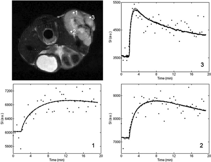
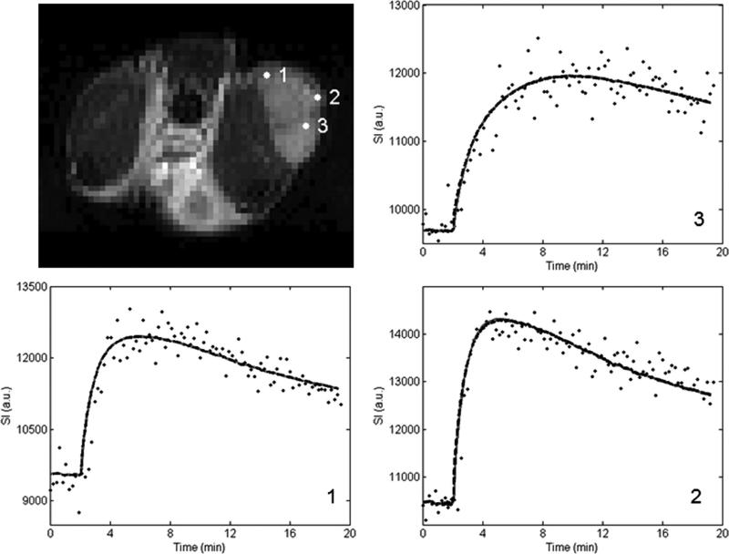
Figures 1 and 2 show representative pixel fits for the standard and extended model analyses for the 128² and 64² acquisition, respectively. The top left panel shows the T₂-weighted anatomical image and the three remaining panels show the voxel signal intensity curves with their corresponding standard and extended model fits. The acquired voxel signal values are represented by the black dots, the standard model fits are shown as the gray solid lines, and the extended model fits are given by the black dashed lines. The number in the lower right-hand corner of each graph corresponds to the numbered point on the anatomical figure. In all cases, the difference between the chi square values for the standard and extended models is less than 3%, indicating great similarity between the two models’ ability to describe the data.

FIG. 1.

Voxel signal intensity data and the associated standard and extended model fits from various locations within the tumor. The data set utilized is from the 128² acquisition, and the number on the curve panels corresponds to the numbered marker on the tumor volume in the top left panel. The standard model fit is represented by the gray solid line and the extended model fit is shown as the black dashed line.

FIG. 2.

This figure presents the 64 × 64 data corresponding to that presented in Figure 1.

Standard Model

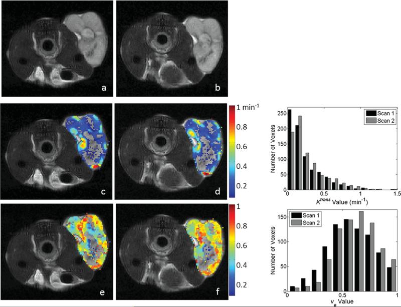
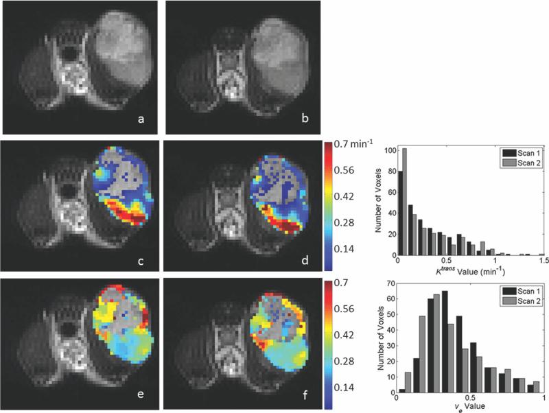
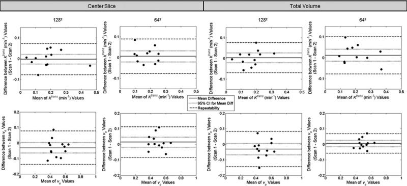
Twelve animals were used for both the 128² acquisition and the 64² analysis. Representative parameter maps for scans 1 and 2 of the 128² and 64² acquisitions are shown in Figs. 3 and 4, respectively. Both figures are arranged such that the scan 1 data are in the left column and the scan 2 data are in the center column. Each figure has the T₂-weighted anatomical image in the top row, the K^trans parameter map in the middle row and the v_e map in the bottom. In each panel, if the parameter value of a voxel within the ROI was not within the physiologically reasonable range (and therefore not used in the reproducibility analysis), then the voxel was represented in the image with the corresponding gray scale data from the T₂ image. Histograms showing the distribution of parameter values in the ROI are given in the right column of Figs. 3 (128²) and 4 (64²). Figure 5 contains Bland–Altman plots for each parameter. The data for the center slice analysis is given in the first two columns, with the 128² acquisition in the left column and the 64² acquisition in the right column. The total volume data is shown in the last two columns, again with the data for the 128² acquisition on the left and the 64² acquisition on the right. For the center slice analysis, the average median values for K^trans and v_e were 0.16 min^–1 and 0.48, respectively, for the 128² set, and 0.22 min^–1 and 0.49, respectively, for the 64² set. For the total volume analysis, the average median values for K^trans and v_e were 0.17 min^–1 and 0.49, respectively, for the 128² set, and 0.25 min^–1 and 0.50, respectively, for the 64² set. The plots also include the mean difference for the population, which is shown by the solid black line. The 95% CI on the mean is given by the dotted line, and all parameters have a CI which includes zero. The 95% CIs on the mean for the center slice analysis for the 128² acquisition are –0.0025 to +0.0025 min^–1 and –0.058 to +0.012 for K^trans and v_e, respectively, whereas the values for the 64² acquisition are –0.021 to +0.033 min^–1 and –0.018 to +0.046 for K^trans and v_e, respectively. For the total volume analysis, the 95% CIs on the mean for the 128² acquisition are –0.0021 to +0.0027 min^–1 and –0.070 to +0.004 for K^trans and v_e, respectively, whereas the values for the 64² acquisition are –0.017 to +0.041 min^–1 and –0.015 to +0.025 for K^trans and v_e, respectively. The repeatability index is displayed as the dashed line in the figures, the magnitude of which is 0.076 min^–1 and 0.107 for K^trans and v_e, respectively, for the 128² acquisition for the center slice analysis, and 0.083 min^–1 and 0.099 for K^trans and v_e, respectively, in the 64² case. In the total volume analysis, the repeatability index is 0.073 min^–1 and 0.113 for K^trans and v_e, respectively, for the 128² acquisition, and 0.089 min^–1 and 0.063 for K^trans and v_e, respectively, in the 64² case.

FIG. 3.

Representative parameter maps and corresponding histograms of the center slice from the 128² test–retest acquisitions as evaluated by the standard model. Parameter values were calculated in the tumor ROI and overlaid on a T₂-weighted anatomical image (a,b). Panels (c) and (d) demonstrate K^trans values for scans 1 and 2, respectively. Panels (e) and (f) demonstrate v_e values corresponding to scans 1 and 2, respectively. Voxels with parameter values outside of the acceptable range (see text) were replaced in the images with the corresponding T₂ gray scale value. Similar parameter patterns and spatial distributions of high and low values are observed between scans; the degree of agreement is demonstrated in the histograms in the right column. The top histogram represents the distribution of K^trans values for scans 1 (black bars) and 2 (gray bars), whereas the bottom histogram displays the analogous data for v_e. [Color figure can be viewed in the online issue, which is available at wileyonlinelibrary.com.]

FIG. 4.

Representative parameter maps of the center slice from the 64² reproducibility acquisition as evaluated by the standard model, and corresponding histograms for parameter distribution. The data in each panel corresponds to that displayed in the 128 × 128 data of Figure 3. As was the case in the 128² acquisition, similar parameter patterns and spatial distributions of high and low values are observed between scans. The corresponding histograms demonstrating the degree of parameter agreement are shown in the right column. [Color figure can be viewed in the online issue, which is available at wileyonlinelibrary.com.]

FIG. 5.

Differences between parameter values for the two scans plotted against the mean value of the scans in the standard model analysis. Plots are shown for both the center slice (left two columns) and the whole tumor volume analyses (right two columns). For each analysis, data for the 128² acquisition are in the left column, whereas data for the 64² acquisition are in the right. In all cases, K^trans is shown in the top row, whereas v_e is on the bottom. The parameter value for each scan is calculated as the median of the parameter values within the ROI. The mean difference is shown by the solid line and the 95% CI on the mean is displayed by the dotted line. The repeatability value is shown by the dashed line. The value for each measure for each parameter, as well as its interpretation, is provided in the text.

The reproducibility statistics for the standard model analysis are tabulated in Table 1 for the center slice analysis and Table 2 for the total volume analysis. For all parameters except K^trans (center slice analysis, 64² acquisition), the distribution of d was not significantly different from normal (Shapiro–Wilk, P > 0.05). Additionally, we detected no statistically significant dependence between d and the average of the two repeat tests for any parameter (Kendall's tau, P > 0.05). Tables 1 and 2 contain data for the mean parameter value, mean difference, the precision (1/2 of the 95% CI) for the mean, within-patient standard deviation (wSD), within-patient coefficient of variation (wCV), and repeatability index for each parameter. The 95% CIs for the mean difference all contain zero suggesting unbiased reproducibility. For both the center slice analysis and the total volume analysis, K^trans is more reproducible in the 128² acquisition, whereas v_e has a lower repeatability index for the 64² acquisition. In regards to the center slice analysis versus the total volume analysis, the reproducibility is very comparable, with no observable difference between the two.

Table 1.

Center Slice Reproducibility Statistics for Analysis via the Standard Model and Extended Models for the 128² Acquisition (a and c) and 64² Acquisition (b and d)

Parameter	Mean	Mean difference	95% CI (population)	wSD	wCV (%)	Repeatability
(a) 128 × 128 standard
Ktrans (min–1)	0.156	–0.0002	± 0.025	0.027	17.6	0.076
ve	0.482	–10.023	± 0.035	0.039	8.0	0.107
(b) 64 × 64 standard
Ktrans (min–1)	0.216	0.006	± 0.027	0.030	13.9	0.083
ve	0.491	0.014	± 0.032	0.036	7.3	0.099
(c) 128 × 128 extended
Ktrans (min–1)	0.115	–0.006	± 0.017	0.020	17.4	0.055
ve	0.510	–0.010	± 0.025	0.028	5.6	0.079
vp	0.029	–0.003	± 0.003	0.004	11.8	0.010
(d) 64 × 64 extended
Ktrans (min–1)	0.152	–0.005	± 0.023	0.025	16.6	0.070
ve	0.520	0.032	± 0.028	0.031	6.0	0.087
vp	0.022	0.0003	± 0.003	0.004	17.0	0.010

Table 2.

Total Volume Reproducibility Statistics for Analysis via the Standard Model and Extended Models for the 128² Acquisition (a and c) and 64² Acquisition (b and d)

Parameter	Mean	Mean difference	95% CI (population)	wSD	wCV (%)	Repeatability
(a) 128 × 128 standard
Ktrans (min–1)	0.168	0.003	± 0.024	0.026	15.6	0.073
ve	0.492	–0.033	± 0.037	0.041	8.3	0.113
(b) 64 × 64 standard
Ktrans (min–1)	0.245	0.012	± 0.029	0.032	13.2	0.089
ve	0.502	0.005	± 0.020	0.023	4.5	0.063
(c) 128 × 128 extended
Ktrans (min–1)	0.128	0.010	± 0.024	0.027	21.2	0.075
ve	0.478	–0.021	± 0.022	0.025	5.2	0.069
vp	0.033	–0.003	± 0.005	0.005	15.7	0.014
(d) 64 × 64 extended
Ktrans (min–1)	0.169	0.003	± 0.020	0.023	13.5	0.063
ve	0.527	0.017	± 0.030	0.033	6.2	0.091
vp	0.024	–0.001	± 0.002	0.002	8.4	0.006

Extended Model

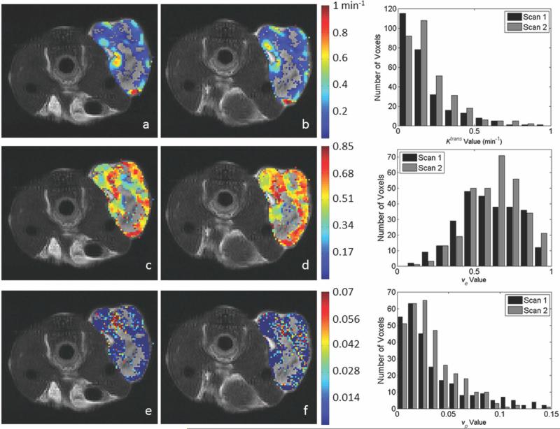
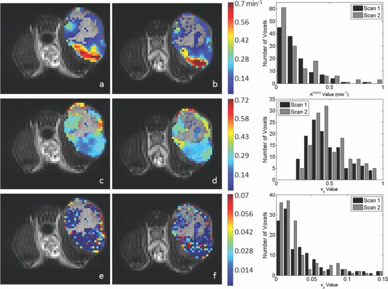
Representative center slice parameter maps from the extended model evaluation are shown for the 128² acquisition and the 64² acquisition in Figs. 6 and 7, respectively. These figures are arranged similar to Figs. 3 and 4, with the exception that K^trans maps are on the top row, v_e maps are in the center row, and v_p maps are on the bottom row. As in the previous figures, if the extended model assigned ROI voxel parameter values that were outside of the designated range for K^trans and v_e, the voxel is represented in the image by the gray scale T₂ value. Though we excluded voxels from the statistical analysis if v_p < 0.001, to enable a visual comparison between the standard and extended model results, we have colored all voxels provided v_p > 0. Note that, overall, there is tremendous agreement between the K^trans and v_e values as estimated by the standard and extended models. In fact, when considering only the voxels for which 0 < v_p < 0.001, the CCC was identically one for both K^trans and v_e and both acquisition matrices. When only the voxels for which v_p > 0.001 are included, the CCC is reduced to 0.84 for K^trans and 0.96 for v_e, though this still indicates a very strong relationship between the parameters returned by the two models. Furthermore, to compare the appropriateness of the standard model versus the extended model in describing the data, we calculated the AIC for each model. In all cases, the AIC was lower for the standard model than for the extended model. We return to this important point in the “Discussion” section.

FIG. 6.

The figure presents data corresponding to that in Figure 3, only here the kinetic analysis is performed with the extended model to return estimates of K^trans, v_e, and v_p. Panels (a) and (b) demonstrate K^trans values for scans 1 and 2, respectively. Panels (c) and (d) demonstrate cCorresponding v_e values for scans 1 and 2, respectively, whereas panels (e) and (f) show corresponding v_p values for scans 1 and 2, respectively. As was the case in the Figs. 3 and 4, voxels with parameter values outside of the acceptable range for K^trans and v_e were replaced in the images with the corresponding T₂ gray scale value. To enable a comparison to the standard model presented in Figure 3, we included voxels for which v_p > 0 (though only v_p > 0.001 values were included in the statistical analysis. Similar parameter patterns and spatial distributions of high and low values are observed between scans; the degree of agreement is demonstrated in the histograms shown the right column. The top histogram represents the distribution of K^trans values for scan 1 (black bars) and 2 (gray bars). The center panel shows the distribution of v_e for scan 1 (black bars) and scan 2 (gray bars), and the bottom histogram gives the distribution of v_p for scans 1 (black bars) and 2 (gray bars). [Color figure can be viewed in the online issue, which is available at wileyonlinelibrary.com.]

FIG. 7.

The data in each panel correspond to that displayed in the 128 × 128 data of Figure 6. Voxels with parameter values outside of the acceptable range for K^trans and v_e were replaced in the images with the corresponding T₂ gray scale value. As was the case in the 128 × 128 images, many voxels had v_p values less than 0.001 and were included from the figure. As was observed in the 128² acquisition, similar parameter patterns and regions of high and low values are identifiable between scans; the degree of agreement is demonstrated in the histograms shown in the right column. [Color figure can be viewed in the online issue, which is available at wileyonlinelibrary.com.]

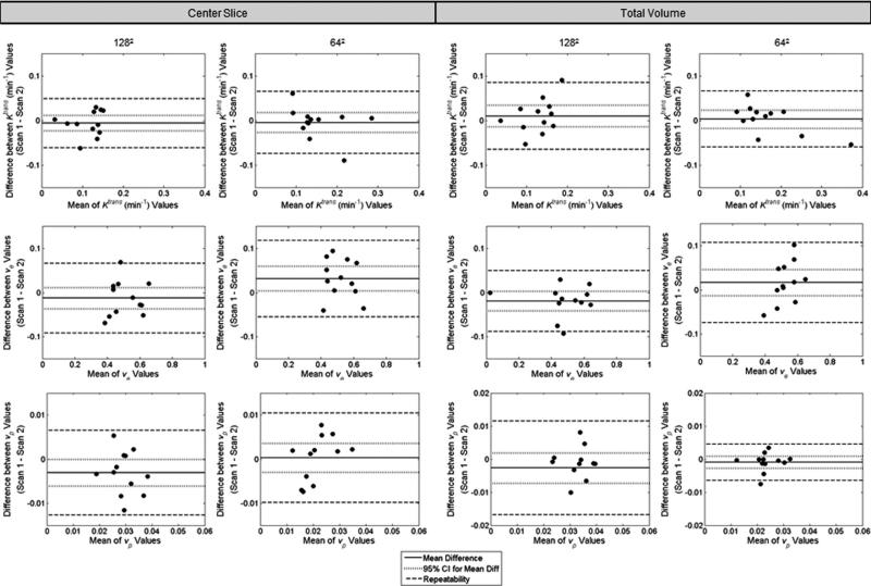
Bland–Altman plots for each parameter are given in Figure 8, with results for the center slice analysis in the left two columns and the results for the total volume analysis in the right two. As before, the 128² acquisition results are on the left, whereas those for the 64² acquisition are on the right. The population mean of the difference is given by the solid line, and the 95% CI range is shown by the dotted line. In the center slice analysis using the extended model, one parameter from the 64² analysis, v_e, had a mean difference that was significantly different from zero (Wilcoxon signed rank test, P <0.05) and a CI that did not include zero. The remaining parameters did not indicate bias (Wilcoxon signed rank test, P >0.05, CI includes zero). The 95% CI values for the center slice analysis are –0.023 to +0.011 min^–1 for K^trans, –0.035 to +0.015 for v_e, and –0.006 to 0 for v_p at the 128² acquisition, and –0.028 to 0.018 min^–1 for K^trans, +0.004 to +0.060 for v_e, and –0.003 to +0.003 for v_p at the 64² acquisition. In the total volume analysis, the 95% CI values are –0.014 to +0.034 min^–1 for K^trans, –0.043 to +0.001 for v_e, and –0.008 to +0.002 for v_p at the 128² acquisition, and –0.017 to 0.023 min^–1 for K^trans, –0.013 to +0.047 for v_e, and –0.003 to +0.001 for v_p at the 64² acquisition. The repeatability index for each parameter is given by the dashed line. Repeatability values are 0.055 min^–1, 0.079, and 0.010 for K^trans, v_e, and v_p, respectively, in the 128² case for the center slice analysis, and 0.070 min^–1, 0.087, and 0.010 for K^trans, v_e, and v_p, respectively, in the 64² case, whereas the repeatability values for the total volume analysis are 0.075 min^–1, 0.069, and 0.014 for K^trans, v_e, and v_p, respectively, in the 128² case for the center slice analysis, and 0.063 min^–1, 0.091, and 0.006 for K^trans, v_e, and v_p, respectively, in the 64² case.

FIG. 8.

The figure displays the extended model version of Figure 5. Differences between parameter values for the two scans plotted against the mean value of the scans in the extended model analysis. Plots are shown for both the center slice analysis (left two columns) and the total volume analysis (right two columns). For each analysis, data for the 128² acquisition is in the left column while data for the 64² acquisition is in the right. In all cases, K^trans is shown in the top row, v_e is in the middle row, and v_p is in the bottom row. The parameter value for each scan is calculated as the median of the parameter values within the ROI. The mean difference is shown by the solid line and the 95% CI on the mean is displayed by the dotted line. The repeatability value is shown by the dashed line. The value for each measure for each parameter, as well as its interpretation, is provided in the text.

The reproducibility statistics for the extended model analysis are compiled in Tables 1 and 2. Three parameters demonstrated a potential non-normal distribution (Shapiro–Wilk, P < 0.05): v_p in the center slice analysis of the 128² acquisition, v_e in the center slice analysis of the 64² acquisition, and K^trans in the total volume analysis of the 128² acquisition. For the remaining parameters, the assumption of normality could not be rejected (Shapiro–Wilk, P > 0.05). No parameter had a statistically significant correlation between d and the mean of the paired values (Kendall's tau, P > 0.05). The mean values for the 128² acquisition are 0.12 min^–1, 0.51, and 0.029 for K^trans, v_e, and v_p, respectively, in the center slice analysis and 0.13 min^–1, 0.48, and 0.033 for K^trans, v_e, and v_p, respectively, in the total volume analysis. The mean values for the 64² acquisition for the center slice analysis are 0.15 min^–1 for K^trans, 0.52 for v_e, and 0.022 for v_p. For the total volume analysis of the 64² acquisition, the mean values are 0.17 min^–1 for K^trans, 0.53 for v_e, and 0.024 for v_p. The tables also give the mean difference, precision (1/2 of the 95% CI), wSD, wCV, and repeatability for each parameter. As for the standard model, there is no appreciable difference between the center slice analysis and the total tumor volume analysis for the extended model. Similarly, the 128² acquisition and the 64² acquisition have very comparable repeatability indices for all parameters.

iAUC

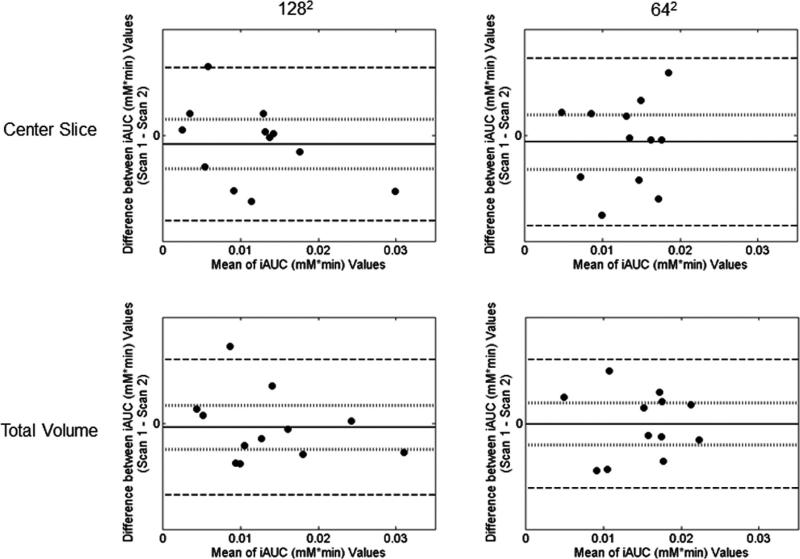
Bland–Altman plots for the iAUC analysis are given in Figure 9. The results are shown for the center slice analysis for the 128² acquisition (top left panel) and the 64² acquisition (top right panel) as well as for the total tumor volume analysis for the 128² acquisition (bottom left panel) and the 64² acquisition (bottom right panel). The population mean of the difference is given by the solid line, and the 95% CI range is shown by the dotted line. For the 128² analysis, the 95% CI is –0.0021 to +0.0013 mM min in the center slice analysis and –0.0012 to 0.0014 mM min in the total tumor volume analysis. For the 64² acquisition, the 95% CI values are –0.0019 to +0.0009 mM min for the center slice analysis and –0.0015 to +0.0011 mM min in the total tumor volume analysis.

FIG. 9.

Difference between parameter values for the two scans plotted against the mean value of the two scans for the iAUC analysis. Data for the 128² acquisition are shown in the left column, whereas data for the 64² acquisition are shown in the right. The top two panels give the results for the center slice analysis, whereas the bottom two panels show the total volume analysis.

The reproducibility statistics for the iAUC are given in Table 3. In all cases, the assumption of normality could not be rejected (Shapiro–Wilk, P > 0.05), and no parameter had a statistically significant correlation between d and the mean of the paired values (Kendall's tau, P > 0.05). The mean median iAUC value of the 128² acquisition is 0.013 mM min for the center slice analysis and 0.015 mM min for the total tumor volume analysis. The mean value for the 64² acquisition is 0.012 and 0.014 mM min for the center slice analysis and the total tumor volume analysis, respectively. The repeatability index is 0.0051 mM min for the 128² acquisition and 0.0043 mM min for the 64² acquisition for the center slice analysis, and 0.0039 mM min for the 128² acquisition and 0.0042 mM min for the 64² acquisition in the total tumor volume analysis. Once again, the reproducibility parameters for the two different acquisition matrices are very similar.

Table 3.

Center Slice and Total Volume Reproducibility Statistics for the iAUC Analysis

Parameter	Mean	Mean difference	95% CI (population)	wSD	wCV (%)	Repeatability
(a) 128 × 128
Center slice (mM min)	0.0130	–0.0004	± 0.0017	0.0019	14.2	0.0051
Total volume (mM min)	0.0150	0.0001	± 0.0013	0.0014	9.5	0.0039
(b) 64 × 64
Center slice (mM min)	0.0116	–0.0005	± 0.0014	0.0016	13.4	0.0043
Total volume (mM min)	0.0137	–0.0002	± 0.0013	0.0015	11.0	0.0042

DISCUSSION

We chose to calculate the group and individual statistics in a manner similar to that outlined by Galbraith et al. (19), which is based on the reproducibility statistics defined by Bland and Altman (34). This analysis provides statistics that allow comparison of reproducibility between parameters as well as define the range of repeatability by quantifying the maximum difference expected to be observed between scans on an individual. Additionally, the 95% CIs for the mean differences reveals whether statistically significant systematic bias is present (e.g., order of measurement is important) in repeat measurements in the same individual. According to our results displayed in Table 1 (center slice analysis) and Table 2 (total tumor volume analysis), we would need to see a change of –0.025 to +0.025 min^–1 for K^trans in the standard model at the 128² resolution in the center slice to denote a significant change. Similarly for the whole tumor analysis, changes of –0.0021 to +0.027 min^–1 for K^trans would need to be observed in a group to denote significance. Results for other parameters are interpreted similarly. In this work, we detected statistically significant systematic bias in v_e in the center slice analysis of the 64² acquisition as fit by the extended model. In this case, the first measurement tended to be higher than the second. Additionally, for four parameters we found that the population may not be normally distributed (Shapiro–Wilk, P < 0.05). However, the analysis implemented here was conservative in testing for significance. For this experiment, if we were to control for type 1 error and applied the Holm–Bonferroni method, the data neither would demonstrate significant systematic bias nor would the assumption of normality be rejected. The repeatability value index suggests the parameter value change for an individual that would be considered an outlier or rare event, as 95% of individual parameter values should fall within these limits. For the standard model analysis, at a resolution of 128² and for the center slice analysis, a value 0.076 min^–1 was calculated for K^trans. In the total volume analysis, the repeatability index for K^trans was 0.073 min^–1. Regarding the iAUC data, the repeatability indices for the 128² acquisition were 0.0051 and 0.0039 mM min for the center slice and total volume analyses, respectively. For the 64² acquisition, the repeatability indices were 0.0043 and 0.0042 mM min for the center slice and total volume analyses, respectively. Results for the other parameters are interpreted in a similar manner.

Overall, there is a considerable amount of agreement between the standard and extended model analyses. Specifically, the CCC for K^trans and v_e between the standard and the extended model values is identically 1 for voxels with v_p values less than 0.001, and 0.84 (K^trans) and 0.96 (v_e) when voxels with v_p greater than 0.001 are considered. This is further indicated by the voxel fits shown in Figs. 1 and 2; in all panels of these figures, the standard and extended model fits overlay almost exactly, again showing the parameter agreement between the two models (for the two parameters common to both models, K^trans and v_e). Thus, it is not surprising that the AIC calculations are uniformly lower for the standard model than for the extended model (as the AIC incorporates a penalty for additional model parameters) thereby indicating that the standard model is the most parsimonious for these data sets. This is further validated qualitatively by the fact that the majority of the voxels have very low (if not approaching 0) values of v_p. This apparent lack of vascularity in the tumor model could also be attributed to a limitation of the imaging protocol; specifically, the bolus injection of the contrast agent. Though the contrast agent injection was uniformly performed in all studies by an automatic injector, given confounding factors such as the small blood volume of the mouse (~2 mL) and the relative coarseness of the time discretization in the DCE acquisition protocol, it is possible that the first pass of the contrast agent is lost in the data, thus limiting the power of the extended model in describing these data sets. However, in those voxels for which v_p > 0.001 the statistics for the extended model are valid and provide some much needed data on the reproducibility of the extended model in mouse models of cancer. In particular, the data should be of some use when applying the extended model to mouse cancer systems that display high blood volumes throughout the tumor. In practice, we recommend that DCE-MRI data sets be analyzed with both models and use the AIC (or other suitable metric) to determine which method is appropriate for the particular animal system under investigation.

To the best of our knowledge, this is the first study attempting to quantify the reproducibility of DCE-MRI in a murine model of cancer, and hence there is no data available to which we can directly compare these results. The work by McGrath et al. provided data on the reproducibility of the extended model analysis in a rat model of cancer, thus providing the most comparable data to the work presented here (24). For the population AIF, the authors found mean differences of 3.57% for K^trans, 3.58% for v_e, and –26.22% for v_p. Additionally, the 95% CIs are approximately –10 to 20% for K^trans, –8 to 15% for v_e, and 60 to 5% for v_p. The data are most comparable to our center slice analysis of the 128² acquisition. In our work, the mean differences (as a percentage of the mean parameter value) were –5.4% for K^trans, –2.0% for v_e, and –10.3% for v_p, and the 95% CIs (again as a percentage of the mean parameter value) were –20.4 to 9.6% for K^trans, –6.8 to 2.8% for v_e, and –20.5 to 0% for v_p. Thus, the results presented here are very similar to those presented by McGrath et al. (24). In regards to clinical data, it is difficult to directly compare this work to human studies given the limitations imposed by differences in experimental design. However, the work by Galbraith et al. provides a set of human reproducibility data in the standard model analysis to which we can generally compare our results (19). The authors found 95% CIs of –14 to +16% for K^trans and ±6% for v_e. The repeatability indices were –45 to 83% for K^trans and 24% (as a percentage of mean parameter value) for v_e. The results are most comparable to our center slice analysis of the 64² acquisition; here, we found CIs of ±13% for K^trans and ±7% for v_e, and the repeatability indices were 38% (of the mean parameter) for K^trans and 20% for v_e. Thus, the results presented here are comparable to those shown in the work by Galbraith et al. (19)

Though we attempted to be as consistent as possible in conducting this study, it is not without its limitations. Perhaps the most prominent issue is that we are not comparing exactly the same section of tissue between scans. We chose to remove the animal between scans to simulate the repositioning of an animal that would occur during a treatment study, thus allowing us to generate reproducibility statistics in terms of what we would expect to see in a treatment study. Additionally, allowing the animal to recover eliminates any physiological stress that may occur during, say, a 5-h period of anesthesia. However, this also means that there would be slight differences between the tissue ROIs investigated in the first scan versus the second scan, due to repositioning errors. We would expect the errors associated with repositioning to reduce the reproducibility of our scans (or effectively increase the magnitude of the repeatability value). A second limitation of the work is the use of the population AIF for the data analysis. The use of the population AIF is eminently practical due to the difficulties associated with attempting to derive an individual AIF in a murine subject. Though the population AIF that we utilized was rigorously obtained and studied (14), its use can still introduce errors due to subtle variations in animal physiology.

CONCLUSIONS

Quantitative imaging biomarkers have the potential to be more sensitive to early treatment-driven changes in the tumor microenvironment than current, macroscopically driven anatomic assessment methods. However, before such quantitative techniques, like DCE-MRI, can be employed in either preclinical or clinical studies of treatment efficacy, the reproducibility must be assessed. The present effort focused on evaluating the reproducibility of DCE-MRI in the preclinical setting, utilizing a murine model of HER2+ breast cancer. The results provide values that define significant changes in an individual and a group analysis in a variety of analysis regimens for both quantitative and semiquantitative parameters. Thus, this work defines a foundation for moving forward in investigating the use of DCE-MRI for assessing treatment response.

REFERENCES

- 1.Lemasson B, Christen T, Tizon X, et al. Assessment of multiparametric MRI in a human glioma model to monitor cytotoxic and anti-angiogenic drug effects. NMR Biomed. 2011;24:473–482. doi: 10.1002/nbm.1611. [DOI] [PMC free article] [PubMed] [Google Scholar]
- 2.Wang H, Cona MM, Chen F, Yu J, Feng Y, Li J, de Keyzer F, Marchal G, Ni Y. Comparison of two vascular-disrupting agents at a clinically relevant dose in rodent liver tumors with multiparametric magentic resonance imaging biomarkers. Anti-Cancer Drugs. 2012;23:12–21. doi: 10.1097/CAD.0b013e328349dd60. [DOI] [PubMed] [Google Scholar]
- 3.O'Connor JPB, Rose CJ, Jackson A, et al. DCE-MRI biomarkers of tumour heterogeneity predict CRC liver metastasis shrinkage following bevacizumab and FOLFOX-6. Br J Cancer. 2011;105:139–145. doi: 10.1038/bjc.2011.191. [DOI] [PMC free article] [PubMed] [Google Scholar]
- 4.Ah-See M, Makris A, Taylor NJ, et al. Early changes in functional dynamic magnetic resonance imaging predict for pathologic response to neoadjuvant chemotherapy in primary breast cancer. Clinical Cancer Res. 2008;14:6580–6589. doi: 10.1158/1078-0432.CCR-07-4310. [DOI] [PubMed] [Google Scholar]
- 5.Kelly RJ, Rajan A, Force J, et al. Evaluation of KRAS mutations, angiogenic biomarkers and DCE-MRI in patients with advanced no-small-cell lung cancer receiving sorafenib. Clin Cancer Res. 2011;17:1190–1199. doi: 10.1158/1078-0432.CCR-10-2331. [DOI] [PMC free article] [PubMed] [Google Scholar]
- 6.Shah C, Miller TW, Wyatt SK, et al. Imaging biomarkers predict response to anti-HER2 (ErbB2) therapy in preclinical models of breast cancer. Clin Cancer Res. 2009;15:4712–4721. doi: 10.1158/1078-0432.CCR-08-2635. [DOI] [PMC free article] [PubMed] [Google Scholar]
- 7.Sharma U, Danishad KKA, Seenu V, Jagannathan NR. Longitudinal study of the assessment by MRI and diffusion-weighted imaging of tumor response in patients with locally advanced breast cancer undergonig neoadjuvant chemotherapy. NMR Biomed. 2009;22:104–113. doi: 10.1002/nbm.1245. [DOI] [PubMed] [Google Scholar]
- 8.Yang M, Gao H, Yan Y, Sun X, Chen K, Quan Q, Lang L, Kiesewetter D, Niu G, Chen X. PET imaging of early response to the tyrosine kinase inhibitor ZD4190. Eur J Nucl Med Mol Imaging. 2011;38:1237–1247. doi: 10.1007/s00259-011-1742-z. [DOI] [PMC free article] [PubMed] [Google Scholar]
- 9.Pope WB, Kim HJ, Huo J, et al. Recurrent glioblastoma multiforme: ADC histogram analysis predicts response to bevacizumab treatment. Radiology. 2009;252:182–189. doi: 10.1148/radiol.2521081534. [DOI] [PubMed] [Google Scholar]
- 10.Li SP, Makris A, Beresford MJ, Taylor NJ, Ah-See M, Stirling JJ, d'Arcy JA, Collins DJ, Kozarski R, Padhani AR. Use of dynamic contrast-enhanced MR imaging to predict survival in patients with primary breast cancer undergoing neoadjuvant chemotherapy. Radiology. 2011;260:68–78. doi: 10.1148/radiol.11102493. [DOI] [PubMed] [Google Scholar]
- 11.Loveless ME, Lawson D, Collins M, Nadella MV, Reimer C, Huszar D, Halliday J, Waterton JC, Gore JC, Yankeelov TE. Comparisons of the efficacy of a Jak1/2 inhibitor (AZD1480) with a VEGF signaling inhibitor (cediranib) and sham treatments in mouse tumors using DCE-MRI, DW-MRI, and histology. Neoplasia. 2012;14:54–64. doi: 10.1593/neo.111478. [DOI] [PMC free article] [PubMed] [Google Scholar]
- 12.Eisenhauer E, Therasse P, Boggaerts J, et al. New response evaluation criteria in solid tumours: revised RECIST guideline (version 1.1). Eur J Cancer. 2009;45:228–247. doi: 10.1016/j.ejca.2008.10.026. [DOI] [PubMed] [Google Scholar]
- 13.Yankeelov TE, Gore JC. Dynamic contrast enhanced magnetic resonance imaging in oncology: theory, data, acquisition, analysis, and examples. Curr Med Imaging Rev. 2007;3:91–107. doi: 10.2174/157340507780619179. [DOI] [PMC free article] [PubMed] [Google Scholar]
- 14.Loveless M, Halliday J, Liess C, Xu L, Dortch R, Whisenant J, Water-ton J, Gore J, Yankeelov T. A quantitative comparison of the influence of individual versus population-derived vascular input functions on a dynamic contrast enhanced-MRI in small animals. Magn Reson Med. 2012;67:226–236. doi: 10.1002/mrm.22988. [DOI] [PMC free article] [PubMed] [Google Scholar]
- 15.Pickup S, Zhou R, Glickson J. MRI estimation of the arterial input function in mice. Acad Radiol. 2003;10:963–968. doi: 10.1016/s1076-6332(03)00291-5. [DOI] [PubMed] [Google Scholar]
- 16.Zhou R, Pickup S, Yankeelov TE, Springer J, C S, Glickson JD. Simultaneous measurement of arterial input function and tumor pharmacokinetics in mice by dynamic contrast enhanced imaging: effects of transcytolemmal water exchange. Magn Reson Med. 2004;52:248–257. doi: 10.1002/mrm.20143. [DOI] [PubMed] [Google Scholar]
- 17.Checkley D, Tessier JJL, Wedge SR, Dukes M, Kendrew J, Curry B, Middleton B, Waterton JC. Dynamic contrast-enhanced MRI of vascular changes induced by the VEGF-signalling inhibitor ZD4190 in human tumour xenografts. Magn Reson Imaging. 2003;21:475–482. doi: 10.1016/s0730-725x(02)00644-6. [DOI] [PubMed] [Google Scholar]
- 18.Heilmann M, Walczak C, Vautier J, Dimicoli J- L, Thomas CD, Lupu M, Mispelter J, Volk A. Simultaneous dynamic T1 and T2* measurement for AIF assessment combined with DCE MRI in a mouse tumor model. Magn Reson Mater Phys Biol Med. 2007;20:193–203. doi: 10.1007/s10334-007-0082-2. [DOI] [PubMed] [Google Scholar]
- 19.Galbraith SM, Lodge MA, Taylor NJ, Rustin GJS, Bentzen S, Stirling JJ, Padhani AR. Reproducibility of dynamic contrast-enhanced MRI in human muscle and tumours: comparison of quantitative and semi-quantitative analysis. NMR Biomed. 2002;15:132–142. doi: 10.1002/nbm.731. [DOI] [PubMed] [Google Scholar]
- 20.Padhani AR, Hayes C, Landau S, Leach MO. Reproducibility of quantitative dynamic MRI or normal human tissues. NMR Biomed. 2001;15:143–153. doi: 10.1002/nbm.732. [DOI] [PubMed] [Google Scholar]
- 21.Jackson A, Jayson GC, Li KL, Zhu XP, Checkley DR, Tessier JJL, Water-ton JC. Reproducibility of quantitative dynamic contrast-enhanced MRI in newly presenting glioma. Br J Radiol. 2003;76:153–162. doi: 10.1259/bjr/70653746. [DOI] [PubMed] [Google Scholar]
- 22.Morgan B, Utting JF, Higginson A, Thomas AL, Steward WP, Horsfield MA. A simple, reproducible method for monitoring the treatment of tumours using dynamic contrast-enhanced MR imaging. Br J Cancer. 2006;94:1420–1427. doi: 10.1038/sj.bjc.6603140. [DOI] [PMC free article] [PubMed] [Google Scholar]
- 23.Laarhoven HWM, Rijpkema M, Punt CJA, Ruers TJ, Hendriks JCM, Barentsz JO, Heerschap A. Method for quantitation of dynamic MRI contrast agent uptake in colorectal liver metastases. J Magn Reson Imaging. 2003;18:315–320. doi: 10.1002/jmri.10370. [DOI] [PubMed] [Google Scholar]
- 24.McGrath DM, Bradley DP, Tessier JL, Lacey T, Taylor CJ, Parker GJM. Comparison of model-based arterial input functions for dynamic contrast-enhanced MRI in tumor bearing rats. Magn Reson Med. 2009;61:1173–1184. doi: 10.1002/mrm.21959. [DOI] [PubMed] [Google Scholar]
- 25.Ritter CA, Perez-Torres M, Rinehart C, Guix M, Dugger T, Engelman JA, Arteaga CL. Human breast cancer cells selected for resistance to trastuzumab in vivo overexpress epidermal growth factor receptor and ErbB Ligands and remain dependent on the ErbB receptor network. Clin Cancer Res. 2007;13:4909–4919. doi: 10.1158/1078-0432.CCR-07-0701. [DOI] [PubMed] [Google Scholar]
- 26.Landis C, Li X, Telang F, Coderre J, Micca P, Rooney W, Latour L, Vetek G, Palyka I, Jr, Springer CS. Determination of the MRI contrast agent concentration time course in vivo following bolus injection: effect of equilibrium transcytolemmal water exchange. Magn Reson Med. 2000;44:563–574. doi: 10.1002/1522-2594(200010)44:4<563::aid-mrm10>3.0.co;2-#. [DOI] [PubMed] [Google Scholar]
- 27.Tofts PS, Brix G, Buckley DL, et al. Estimating kinetic parameters from dynamic contrast-enhanced T1-weighted MRI of a diffusable tracer: standardized quantities and symbols. J Magn Reson Imaging. 1999;10:223–232. doi: 10.1002/(sici)1522-2586(199909)10:3<223::aid-jmri2>3.0.co;2-s. [DOI] [PubMed] [Google Scholar]
- 28.Daldrup H, Shames D, Wendland M, Okuhata Y, Link T, Rosenau W, Lu Y, Brasch R. Correlation of dynamic contrast-enhanced MR imaging with histologic tumor grade: comparison of macromolecular and small-molecular contrast media. Am J Roentgenol. 1998;171:941–949. doi: 10.2214/ajr.171.4.9762973. [DOI] [PubMed] [Google Scholar]
- 29.de Lussanet Q, Beets-Tan R, Backes W, van der Schaft D, van Engels-hoven J, Mayo K, Griffioen A. Dynamic contrast-enhanced magnetic resonance imaging at 1.5 Tesla with gadopentetate dimeglumine to assess the angiostatic effects of anginex in mice. Eur J Cancer. 2004;40:1262–1268. doi: 10.1016/j.ejca.2004.01.020. [DOI] [PubMed] [Google Scholar]
- 30.Akaike H. A new look at the statistical model identification. IEEE Trans Automatic Control. 1974;19:716–723. [Google Scholar]
- 31.Naish JH, Kershaw LE, Buckley DL, Jackson A, Waterton JC, Parker GJM. Modeling of contrast agent kinetics in the lung using T1-weighted dynamic contrast-enhanced MRI. Magn Reson Med. 2009;61:1507–1514. doi: 10.1002/mrm.21814. [DOI] [PubMed] [Google Scholar]
- 32.Brix G, Zwick S, Kiessling F, Griebel J. Pharmacokinetic analysis of tissue microcirculation using nested models: multimodel inference and parameter identifiability. Med Phys. 2009;36:2923–2933. doi: 10.1118/1.3147145. [DOI] [PMC free article] [PubMed] [Google Scholar]
- 33.Li X, Welch EB, Chakravarthy AB, et al. Statistical comparison of dynamic contrast-enhanced MRI pharmacokinetic models in human breast cancer. Magn Reson Med. 2012;68:261–271. doi: 10.1002/mrm.23205. [DOI] [PMC free article] [PubMed] [Google Scholar]
- 34.Bland JM, Altman DG. Measuring agreement in method comparison studies. Stat Methods Med Res. 1999;8:135–160. doi: 10.1177/096228029900800204. [DOI] [PubMed] [Google Scholar]