Spiked Dirichlet Process Prior for Bayesian Multiple Hypothesis Testing in Random Effects Models

Abstract

We propose a Bayesian method for multiple hypothesis testing in random effects models that uses Dirichlet process (DP) priors for a nonparametric treatment of the random effects distribution. We consider a general model formulation which accommodates a variety of multiple treatment conditions. A key feature of our method is the use of a product of spiked distributions, i.e., mixtures of a point-mass and continuous distributions, as the centering distribution for the DP prior. Adopting these spiked centering priors readily accommodates sharp null hypotheses and allows for the estimation of the posterior probabilities of such hypotheses. Dirichlet process mixture models naturally borrow information across objects through model-based clustering while inference on single hypotheses averages over clustering uncertainty. We demonstrate via a simulation study that our method yields increased sensitivity in multiple hypothesis testing and produces a lower proportion of false discoveries than other competitive methods. While our modeling framework is general, here we present an application in the context of gene expression from microarray experiments. In our application, the modeling framework allows simultaneous inference on the parameters governing differential expression and inference on the clustering of genes. We use experimental data on the transcriptional response to oxidative stress in mouse heart muscle and compare the results from our procedure with existing nonparametric Bayesian methods that provide only a ranking of the genes by their evidence for differential expression.

1 Introduction

This paper presents a semiparametric Bayesian approach to multiple hypothesis testing in random effects models. The model formulation borrows strength across similar objects (here, genes) and provides probabilities of sharp hypotheses regarding each object.

Much of the literature in multiple hypothesis testing has been driven by DNA microarrays studies, where gene expression of tens of thousands of genes are measured simultaneously (Dudoit et al. 2003). Multiple testing procedures seek to ensure that the family-wise error rate (FWER) (e.g., Hochberg (1988), Hommel (1988), Westfall and Young (1993)), the false discovery rate (FDR) (e.g., Benjamini and Hochberg (1995), Storey (2002), Storey (2003), and Storey et al. (2004)), or similar quantities (e.g., Newton et al. (2004)) are below a nominal level without greatly sacrificing power. Accounts on the Bayesian perspective to multiple testing are provided by Berry and Hochberg (1999) and Scott and Berger (2006).

There is a great variety of modeling settings that accommodate multiple testing procedures. The simplest approach, extensively used in the early literature on microarray data analysis, is to apply standard statistical procedures (such as the t-test) separately and then combine the results for simultaneous inference (e.g., Dudoit et al. 2002). Westfall and Wolfinger (1997) recommended procedures that incorporate dependence. Baldi and Long (2001), Newton et al. (2001), Do et al. (2005) and others have sought prior models that share information across objects, particularly when estimating object-specific variance across samples. Yuan and Kendziorski (2006) use finite mixture models to model dependence. Classical approaches that have incorporated dependence in the analysis of gene expression data include Tibshirani and Wasserman (2006), Storey et al. (2007), and Storey (2007) who use information from related genes when testing for differential expression of individual genes.

Nonparametric Bayesian approaches to multiple testing have also been explored (see, for example, Gopalan and Berry (1998), Dahl and Newton (2007), MacLehose et al. (2007), Dahl et al. (2008)). These approaches model the uncertainty about the distribution of the parameters of interest using Dirichlet process (DP) prior models that naturally incorporate dependence in the model by inducing clustering of similar objects. In this formulation, inference on single hypotheses is typically done by averaging over clustering uncertainty. Dahl and Newton (2007) and Dahl et al. (2008) show that this approach leads to increased power for hypothesis testing. However, the methods provide posterior distributions that are continuous, and cannot therefore be used to directly test sharp hypotheses, which have zero posterior probability. Instead, decisions regarding such hypotheses are made based on calculating univariate scores that are context specific. Examples include the sum-of-squares of the treatment effects (to test a global ANOVA-like hypothesis) and the probability that a linear combination of treatment effects exceeds a threshold.

In this paper we build on the framework of Dahl and Newton (2007) and Dahl et al. (2008) to show how the DP modeling framework can be adapted to provide meaningful posterior probabilities of sharp hypotheses by using a mixture of a point-mass and a continuous distribution as the centering distribution of the DP prior on the coefficients of a random effects model. This modification retains the increased power of DP models but also readily accommodates sharp hypotheses. The resulting posterior probabilities have a very natural interpretation in a variety of uses. For example, they can be used to rank objects and define a list according to a specified expected number of false discoveries. We demonstrate via a simulation study that our method yields increased sensitivity in multiple hypothesis testing and produces a lower proportion of false discoveries than other competitive methods, including standard ANOVA procedures. In our application, the modeling framework we adopt simultaneously infers the parameters governing differential expression and clusters the objects (i.e., genes). We use experimental data on the transcriptional response to oxidative stress in mouse heart muscle and compare results from our procedure with that of existing nonparametric Bayesian methods which only provide a ranking of the genes by their evidence for differential expression.

Recently Cai and Dunson (2007) independently proposed the use of similar spiked priors in DP priors in a Bayesian nonparametric linear mixed model where variable selection is achieved by modeling the unknown distribution of univariate regression coefficients. Similarly, MacLehose et al. (2007) used this formulation in their DP mixture model to account for highly correlated regressors in an observational study. There, the clustering induced by the Dirichlet process is on the univariate regression coefficients and strength is borrowed across covariates. Finally, Dunson et al. (2008) use a similar spiked centering distribution of univariate regression coefficients in a logistic regression. In contrast, our goal is nonparametric modeling of multivariate random effects which may equal the zero vector. That is, we do not share information across univariate covariates but rather seek to leverage similarities across genes by clustering vectors of regression coefficients associated with the genes.

The remainder of the paper is organized as follows. Section 2 describes our proposed modeling framework and the prior model. In Section 3 we discuss the MCMC algorithm for inference. Using simulated data, we show in Section 4.1 how to make use of the posterior probabilities of hypotheses of interest to aid the interpretation of the hypothesis testing results. Section 4.2 describes the application to DNA microarrays. In both Sections 4.1 and 4.2, we compare our proposed method to the LIMMA (Smyth 2004), to the SIMTAC method of Dahl et al. (2008) and to a standard ANOVA procedure. Section 5 concludes the paper.

2 Dirichlet Process Mixture Models for Multiple Testing

2.1 Random Effects Model

Suppose there are K observations on each of G objects and T* treatments. For each object g, with g = 1, …, G, we model the data vector d_g with the following K-dimensional multivariate normal distribution:

$${\mathit{d}}_g\mid {\mu }_g,{\beta }_g,{\lambda }_g\sim {\mathrm{N}}_K({\mathit{d}}_g\mid {\mu }_g\mathit{j}+\mathbf{X}{\beta }_g,{\lambda }_g\mathbf{M}),$$ (1)

where μ_g is an object-specific mean, j is a vector of ones, X is a K × T design matrix, β_g is a vector of T regression coefficients specific to object g, M is the inverse of a correlation matrix of the K observations from an object, and λ_g is an object-specific precision (i.e., inverse of the variance). We are interested in testing a hypothesis for each of G objects in the form:

$$\begin{array}{cc}\hfill & H_{0,g}:{\beta }_{1,g}=\dots ={\beta }_{T^{\ast },g}=0\hfill \\ \hfill & H_{a,g}:{\beta }_{t,g}\ne 0\text{for some}t=1,\dots ,T^{\ast }\hfill \end{array}$$ (2)

for g = 1, …, G.

Object-specific intercept terms are μ_gj, so the design matrix X does not contain the usual column of ones and T is one less than the number of treatments (i.e., T = T* − 1). Also, d₁, …, d_G are assumed to be conditionally independent given all model parameters. In the example of Section 4.2, the objects are genes with d_g being the background-adjusted and normalized expression data for a gene g under T* treatments, G being the number of genes, and K being the number of microarrays. In the example, we have K = 12 since there are 3 replicates for each of T* = 4 treatments, and the X matrix is therefore:

$$\mathbf{X}=\left(\begin{array}{ccc}\hfill 0_3\hfill & \hfill 0_3\hfill & \hfill 0_3\hfill \\ \hfill {\mathit{j}}_3\hfill & \hfill 0_3\hfill & \hfill 0_3\hfill \\ \hfill 0_3\hfill & \hfill {\mathit{j}}_3\hfill & \hfill 0_3\hfill \\ \hfill 0_3\hfill & \hfill 0_3\hfill & \hfill {\mathit{j}}_3\hfill \end{array}\right)$$

where j₃ is a 3-dimensional column vector of ones and 0₃ a 3-dimensional column vector of zeroes. If there are other covariates available, they would be placed as extra columns in X. Note that the design matrix X and the correlation matrix M are known and common to all objects, whereas μ_g, β_g, and λ_g are unknown object-specific parameters. For experimental designs involving independent sampling (e.g., the typical time-course microarray experiment in which subjects are sacrificed rather than providing repeated measures), M is simply the identity matrix.

2.2 Prior Model

We take a nonparametric Bayesian approach to model the uncertainty on the distribution of the random effects. The modeling framework we adopt allows for simultaneous inference on the regression coefficients and on the clustering of the objects (i.e., genes). We achieve this by placing a Dirichlet process (DP) prior (Antoniak 1974) with a spiked centering distribution on the distribution function of the regression coefficient vectors, β₁, …, β_G,

$$\begin{array}{cc}\hfill {\beta }_1,\dots ,{\beta }_G\mid & G_{\beta }\sim G_{\beta }\hfill \\ \hfill & G_{\beta }\sim \mathit{DP}({\alpha }_{\beta },G_{0\beta })\hfill \end{array}$$

where G_β denotes a distribution function of β, DP stands for a Dirichlet process, α_β is a precision parameter, and G_0β is a centering distribution, i.e., E[G_β] = G_0β. Sampling from DP induces ties among β₁, …, β_G, since there is a positive probability that β_i = β_j for every i ≠ j. Two objects i ≠ j are said to be clustered in terms of their regression coefficients if and only if β_i = β_j. The clustering of the objects encoded by the ties among the regression coefficients will simply be referred to as the “clustering of the regression coefficients,” although it should be understood that it is the data themselves that are clustered. The fact that our model induces ties among the regression coefficients β₁, …, β_G is the means by which it borrows strength across objects for estimation.

Set partition notation is helpful throughout the paper. A set partition ξ = {S₁, …, S_q} of S₀ = {1, 2, …, G} has the following properties: Each component S_i is non-empty, the intersection of two components S_i and S_j is empty, and the union of all components is S₀. A cluster S in the set partition ξ for the regression coefficients is a set of indices such that, for all i ≠ j ∈ S, β_i = β_j. Let β_S denote the common value of the regression coefficients corresponding to cluster S. Using this set partition notation, the regression coefficient vectors β₁, …, β_G can be reparametrized as a partition ξ_β and a collection of unique model parameters ϕ_β = (β_S1, …, β_Sq). We will use the terms clustering and set partition interchangeably.

Spiked Prior Distribution on the Regression Coefficients

Similar modeling frameworks and inferential goals to the one we describe in this paper were considered by Dahl and Newton (2007) and Dahl et al. (2008). However, their prior formulation does not naturally permit hypothesis testing of sharp hypotheses, i.e., it can not provide Pr(H_a,g|data) = 1 - Pr(H_0,g|data), where hypotheses are defined as in (2), since the posterior distribution of β_t,g is continuous. Therefore, they must rely on univariate scores capturing evidence for these hypotheses. The prior formulation we adopt below, instead, allows us to estimate the probability of sharp null hypotheses directly from the MCMC samples.

These distributions have been widely used as prior distribution in the Bayesian variable selection literature (George and McCulloch 1993; Brown et al. 1998). Spiked distributions are a mixture of two distributions: the “spike” refers to a point mass distribution at zero and the other distribution is a continuous distribution for the parameter if it is not zero. Here we employ these priors to perform nonparametric multiple hypothesis testing by specifying a spiked distribution as the centering distribution for the DP prior on the regression coefficient vectors β₁, …, β_G. Adopting a spiked centering distribution in DP allows for a positive posterior probability on β_t,g = 0, so that our proposed model is able to provide probabilities of sharp null hypotheses (e.g., H_0,g : β_1,g = … = β_T*,g = 0 for g = 1, …, G) while simultaneously borrowing strength from objects likely to have the same value of the regression coefficients.

We also adopt a “super-sparsity” prior on the probability of β_t,g = 0 (defined as π_t for all g), since it is not uncommon that changes in expressions for many genes will be minimal across treatments. The idea of the “super-sparsity” prior was investigated in Lucas et al. (2006). By using another layer in the prior for π_t, the probability of β_t,g = 0 will be shrunken toward one for genes showing no changes in expressions across treatment conditions.

Specifically, our model uses the following prior for the regression coefficients β₁, …, β_G

$$\begin{array}{cc}\hfill {\beta }_1,\dots ,{\beta }_G\mid G_{\beta }& \sim G_{\beta }\hfill \\ \hfill G_{\beta }& \sim \mathit{DP}({\alpha }_{\beta },G_{0\beta })\hfill \\ \hfill G_{0\beta }& =\prod _{t=1}^T\left\{{\pi }_t{\delta }_0\right({\beta }_{t,g})+(1-{\pi }_t\left)N\right({\beta }_{t,g}\mid m_t,{\tau }_t\left)\right\}\hfill \end{array}$$

$${\pi }_1,\dots ,{\pi }_T\mid {\rho }_1,\dots ,{\rho }_T\sim \prod _{t=1}^T\left\{\right(1-{\rho }_t\left){\delta }_0\right({\pi }_t)+{\rho }_t\mathrm{Beta}(\pi \mid a_{\pi },b_{\pi }\left)\right\}$$

$${\rho }_1,\dots ,{\rho }_T\sim \mathrm{Beta}(\rho \mid a_{\rho },b_{\rho })$$

$${\tau }_1,\dots ,{\tau }_T\sim \mathrm{Gamma}(\tau \mid a_{\tau },b_{\tau })$$

Note that a spiked formulation is used for each element of the regression coefficient vector and π_t = p(β_t,1 = 0) = … = p(β_t,G = 0). Typically, m_t = 0, but other values may be desired. We use the parameterization of the gamma distribution where the expected value of τ_t is a_τb_τ. For simplicity, let π = (π₁, ⋯, π_T) and τ = (τ₁, ⋯, τ_T).

After marginalized over π_t for all t, the G_0β becomes

$$G_{0\beta }=\prod _{t=1}^T\left\{{\rho }_t{r}_{\pi }{\delta }_0\right({\beta }_t)+(1-{\rho }_t{r}_{\pi }\left)N\right({\beta }_t\mid m_t,{\tau }_t\left)\right\},$$

$${\rho }_1,\cdots ,{\rho }_t\sim \mathrm{Beta}(\rho \mid a_{\rho },b_{\rho }).$$

where r_π = a_π/(a_π + b_π). As noted in equation above, the ρ_tr_π is now specified as a probability of β_t,g = 0 for all g.

Prior Distribution on the Precisions

Our model accommodates heteroscedasticity while preserving parsimony by placing a DP prior on the precisions: λ₁, …, λ_G:

$$\begin{array}{cc}\hfill {\lambda }_1,\dots {\lambda }_G\mid G_{\lambda }& \sim G_{\lambda }\hfill \\ \hfill G_{\lambda }& \sim \mathit{DP}({\alpha }_{\lambda },G_{0\lambda })\hfill \\ \hfill G_{0\lambda }& =\mathrm{Gamma}(\lambda \mid a_{\lambda },b_{\lambda })\hfill \end{array}$$

Note that the clustering of the regression coefficients is separate from that of the precisions. Although this treatment for the precisions also has the effect of clustering the data, we are typically more interested in the clustering from the regression coefficients since they capture changes across treatment conditions. We let ξ_λ denote the set partition for the precisions λ₁, …, λ_G and let ϕ_λ = (λ_S1, …, λ_Sq) be the collection of unique precision values.

Prior Distribution on the Precision Parameters for DP

Following Escobar and West (1995), we place independent Gamma priors on the precision parameters α_β and α_λ of the DP priors:

$${\alpha }_{\beta }\sim \mathrm{Gamma}({\alpha }_{\beta }\mid a_{\alpha \beta },b_{\alpha \beta }),$$

$${\alpha }_{\lambda }\sim \mathrm{Gamma}({\alpha }_{\lambda }\mid a_{\alpha \lambda },b_{\alpha \lambda }).$$

Prior Distribution on the Means

We assume a Gaussian prior on the object-specific mean parameters μ₁, …, μ_G:

$${\mu }_g\sim N({\mu }_g\mid m_{\mu },p_{\mu }).$$ (3)

3 Inferential Procedures

In this section, we describe how to conduct multiple hypothesis tests and clustering inference in the context of our model. We treat the object-specific means μ₁, …, μ_G as nuisance parameters since they are not used either in forming clusters or for multiple testing. Thus, we integrate the likelihood with respect to their prior distribution in (3). Simple calculations lead to the following integrated likelihood (Dahl et al. 2008):

$${\mathit{d}}_g\mid {\beta }_g,{\lambda }_g\sim {\mathrm{N}}_K\left({\mathit{d}}_g\mid \mathbf{X}{\beta }_g+{\mathbf{E}}_g^{-1}{\mathit{f}}_g,\frac{{\mathbf{E}}_g}{{\lambda }_g{\mathit{j}}^{\prime }\mathbf{M}\mathit{j}+p_{\mu }}\right),$$ (4)

where

$$\begin{array}{cc}\hfill {\mathbf{E}}_g& ={\lambda }_g({\lambda }_g{\mathit{j}}^{\prime }\mathbf{M}\mathit{j}+p_{\mu })\mathbf{M}-{\lambda }_g^2\mathbf{M}{\mathit{jj}}^{\prime }\mathbf{M},\text{and}\hfill \\ \hfill {\mathit{f}}_g& ={\lambda }_g{m}_{\mu }{p}_{\mu }\mathbf{M}\mathit{j}.\hfill \end{array}$$ (5)

Inference is based on the marginal posterior distribution of the regression coefficients, i.e., p(β₁, …, β_G | d₁, …, d_G) or, equivalently, p(ξ_β, ϕ_β | d₁, …, d_G). This distribution is not available in closed-form, so we use a Markov chain Monte Carlo (MCMC) to sample from the full posterior distribution p(ξ_β, ϕ_β, ϕ_λ, ϕ_λ, ρ, τ | d₁, …, d_G) and marginalize over the parameters ξ_λ, ϕ_λ, ρ, and τ.

3.1 MCMC Scheme

Our MCMC sampling scheme updates each of the following parameters, one at a time: ξ_β, ϕ_β, ξ_λ, ϕ_λ, ρ, and τ. Recall that β_S is the element of ϕ_β associated with cluster S ∈ ξ_β, with β_St being element t of that vector. Likewise, λ_S is the element of ϕ_λ associated with cluster S ∈ ξ_λ. Given starting values for these parameters, we propose the following MCMC sampling scheme. Details for the first three updates are available in the Appendix.

• (1)
  Obtain draws ρ = (ρ₁, …, ρ_T) from its full conditional distribution by the following procedure. First, sample Y_t = r_πρ_t from its conditional distributions:

  $$y_t\mid \cdot \sim p\left(y_t\right)y_t^{\sum _{S\in \xi }I({\beta }_{\mathit{St}}=0)}{(1-y_t)}^{\sum _{S\in \xi }I({\beta }_{\mathit{St}}\ne 0)},$$

  with

  $$p\left(y_t\right)\propto y_t^{a_{\rho }+b_{\rho }-1}{(r_{\pi }-y_t)}^{b_{\rho -1}},$$

  which does not have a known distributional form. A grid-based inverse-cdf method has been adopted for sampling y_t. Once we draw samples of Y_t, then we will obtain ρ_t as Y_t/r_π.
• (2)
  Draw samples of τ = (τ₁, ⋯, τ_T) from their full conditional distributions:

  $${\tau }_t\mid \cdot \sim \mathrm{Gamma}\left(a_{\tau }+\frac{\mid {\zeta }_t\mid }{2},{\left(\frac{1}{b_{\tau }}+\frac{1}{2}\sum _{S\in {\zeta }_t}{({\beta }_{\mathit{St}}-m_t)}^2\right)}^{-1}\right),$$ (6)

  where ζ_t = {S ∈ ξ_β | β_St ≠ 0} and |ζ_t| is its cardinality.
• (3)
  Draw samples of β_S = (β_S1, …, β_ST) for their full conditional distributions:

  $${\beta }_{\mathit{St}}\mid \cdot \sim {\pi }_{\mathit{St}}{\delta }_0+(1-{\pi }_{\mathit{St}})N(h_t^{-1}{z}_t,h_t),$$ (7)

  where

  $$h_t={\tau }_t+\sum _{g\in S}{\mathit{x}}_t^T{\mathit{Q}}_g{\mathit{x}}_t,$$

  $$z_t=m_t{\tau }_t+\sum _{g\in S}{\mathit{x}}_t^T{\mathit{Q}}_g{\mathit{A}}_g,$$

  $${\mathit{Q}}_g={({\lambda }_g{\mathit{j}}^{\prime }\mathit{Mj}+p_{\mu })}^{-1}{\mathit{E}}_g,$$

  $${\mathit{A}}_g={\mathit{d}}_g-{\mathit{X}}_{(-t)}{\beta }_{S(-t)}-{\mathit{E}}_g^{-1}{\mathit{f}}_g,$$

  and the probability π_St is

  $${\pi }_{S_t}=\frac{y_t}{y_t+(1-y_t)\sqrt{h_t^{-1}\tau \exp \{-\frac{1}{2}{\tau }_t{m}_t^2+\frac{1}{2}{h}_t^{-1}{z}_t^2\}}},$$

  where y_t = ρ_tr_π with r_π = a_π/(a_π + b_π), and X_(−t) and β_S(−t) denote the X and β_S with the element t removed, respectively.
• (4)Since a closed-form full conditional for λ_S is not available, update λ_S using a univariate Gaussian random walk.
• (5)Update ξ_β using the Auxiliary Gibbs algorithm (Neal 2000).
• (6)
  Update α_β from its conditional distribution.

  $$\alpha \mid \eta ,k~\{\begin{array}{cc}\mathrm{Gamma}(a_{\alpha }+k,{\beta }_{\alpha }^{\ast })\hfill & \text{with probability}{p}_{\alpha }\hfill \\ \mathrm{Gamma}(a_{\alpha }+k-1,{\beta }_{\alpha }^{\ast })\hfill & \text{with probability}1-p_{\alpha }\hfill \end{array}\phantom{\}}$$

  where

  $$b_{\alpha }^{\ast }={\left(\frac{1}{b_{\alpha }}-\log \left(\eta \right)\right)}^{-1},\text{and}$$

  $$p_{\alpha }=\frac{a_{\alpha }+k-1}{a_{\alpha }+k-1+n∕b_{\alpha }^{\ast }}$$

  Also,

  $$n\mid \alpha ,k~\mathrm{Beta}(\alpha +1,n).$$
• (7)Update ξ_λ using the Auxiliary Gibbs algorithm.
• (8)Update α_λ using the same procedure in (6) above.

3.2 Inference from MCMC Results

Due to our formulation for the centering distribution of the DP prior on the regression coefficients, our model can estimate the probability of sharp null hypotheses, such as H_0,g : β_1,g = ⋯ = β_T*,g = 0 for g = 1, …, G. Other hypotheses may be specified, depending on the experimental goals. We estimate these probabilities by simply finding the relative frequency that the hypotheses hold among the states of the Markov chains.

Our prior model formulation also permits inference on clustering of the G objects. Several methods are available in the literature on DP models to estimate the cluster memberships based on posterior samples. (See, for example, Medvedovic and Sivaganesan 2002; Dahl 2006; Lau and Green 2007.) In the examples below we adopt the least-squares clustering estimation of Dahl (2006) which finds the clustering configuration among those sampled by the Markov chain that minimizes a posterior expected loss proposed by Binder (1978) with equal costs of clustering mistakes.

3.3 Hyperparameters Setting

Our recommendation for setting the hyperparameters is based on computing for each object the least-squares estimates of the regression coefficients, the y-intercept, and the mean-squared error. We then set m_μ to be the mean of the estimated y intercepts and p_μ to be the inverse of their variances. We also use the method of moments to set (a_τ, b_τ). This requires solving the following two equations:

$$a_{\tau }{b}_{\tau }=\text{mean of variance of least-squares regression coefficients}$$

$$a_{\tau }{b}_{\tau }^2=\text{sample variance of variances of least-squares regression coefficients}$$

Likewise, a_λ and b_λ are set using the method of moments estimation, assuming that the inverse of the mean-squared errors are random draws from a gamma distribution having mean a_λb_λ. As for (a_π, b_π) and (a_π, b_π), a specification such that ${\left(r_{\pi }E\right[{\rho }_t\left]\right)}^T={\prod }_{t=1}^{T}p({\beta }_{t,g}=0)=0.50$ is recommended if there is no prior information available.

We refer to these recommended hyperparameter settings as the method of moments (MOM) settings. The MOM recommendations are based on a thorough sensitivity analysis we performed on all the hyperparameters using simulated data. Some results of this simulation study are described in Section 4.1.

4 Applications

We first demonstrate the performance in a simulation study and then apply our method to gene expression data analysis.

4.1 Simulation Study

Data Generation

In an effort to imitate the structure of the microarray data experiment examined in the next section, we generated 30 independent datasets with 500 objects measured at two treatments and three time points, having three replicates at each of the six treatment combinations. Since the model includes an object-specific mean, we set β₆,_g = 0 so that the treatment index t ranges from 1 to 5.

We simulated data in which the regression coefficients β for each cluster is distributed as described in Table 1. Similarly, the three pre-defined precisions λ₁ = 1.5, λ₂ = 0.2 and λ₃ = 3.0 are randomly assigned to each of the 180, 180, and 140 objects (total 500 objects).

Table 1.

Schematic for the simulation of the regression coefficients vectors in the first alternative scenario.

Cluster	Size	β 1	β 2	β 3	β 4	β 5
1	300	0	0	0	0	0
2	50	0	0	$\sim N(0,\frac{1}{4})$	0	$\sim N(0,\frac{1}{4})$
3	50	0	0	0	0	$\sim N(0,\frac{1}{4})$
4	25	$\sim N(0,\frac{1}{4})$	$\sim N(0,\frac{1}{4})$	0	0	0
5	25	0	0	$\sim N(0,\frac{1}{4})$	$\sim N(0,\frac{1}{4})$	0
6	25	$\sim N(0,\frac{1}{4})$	$\sim N(0,\frac{1}{4})$	$\sim N(0,\frac{1}{4})$	$\sim N(0,\frac{1}{4})$	0
7	25	$\sim N(0,\frac{1}{4})$	0	$\sim N(0,\frac{1}{4})$	0	$\sim N(0,\frac{1}{4})$

Sample-specific means μ_g were generated from a univariate normal distribution with mean 10 and precision 0.2. Finally, each vector d_g was sampled from a multivariate normal distribution with mean μ_gj + Xβ_g and precision matrix λ_gI, where I is an identity matrix.

We repeated the procedure above to create 30 independent datasets. Our interest lies in testing the null hypothesis H₀,_g : β₁,_g = … = β₆,_g = 0. All the computational procedures were coded in Matlab.

Results

We applied the proposed method to the 30 simulated datasets. The model involves several hyperparameters: m_μ, p_μ, a_π, b_π, a_ρ, b_ρ, a_τ, b_τ, a_λ, b_λ, a_αβ, b_αβ, a_αλ b_αλ, and We set (a_π, b_π) = (1, 0.15) and (a_ρ, b_ρ) = (1, 0.005). The prior probability of the null hypothesis (i.e., that all the regression coefficients are zero) for an object is about 50%, which is (r_π * E[ρ])⁵ with r_π = a_π/(a_π + b_π) and E[ρ] = a_ρ/(a_ρ + b_ρ), product of Bernoulli random variables across the T treatment conditions each having success probability. We calculated the MOM recommendations from Section 3.3 to set (a_τ, b_τ) and (a_λ, b_λ). These recommendations for the hyperparameters are based on the sensitivity analysis described later in the paper. We somewhat arbitrarily set (a_αβ, b_αβ) = (5, 1) and (a_αβ, b_αβ) = (1, 1), so that prior expected numbers of clusters are about 24 and 7 for the regression coefficients and precisions, respectively. We show the robustness of the choice of those parameters in the later section. For each dataset, we ran two Markov chains for 5,000 iterations and different starting clustering configurations.

A trace plot of the number of clusters of β from the two different starting stages for one of the simulated datasets, as well as a similar plot for λ, is shown in Figure 1. Similar trace plots of generated _αβ and _αλ are shown in Figure 2. They do not indicate any convergence or mixing problems. The other datasets also had plots indicating good mixing. For each chain, we discarded the first 3,000 iterations for a burn-in and pooled the results from the two chains.

Figure 1.

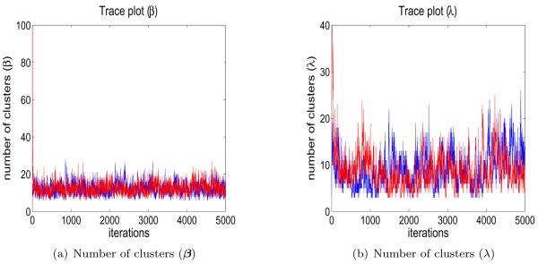
Trace plots of the number of clusters for the regression coefficients and the precisions when fitting a simulated dataset.

Figure 2.

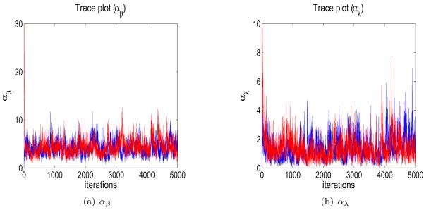
Trace plots of generated α_β and α_λ when fitting a simulated dataset.

Our interest in the study is to see whether there are changes between the two groups within a time point and across time points. Specifically, we considered the null hypothesis that all regression coefficients are equal to zero: for g = 1, …, 500,

$$H_{0,g}:{\beta }_{1,g}=\dots ={\beta }_{6,g}=0$$

$$H_{a,g}:{\beta }_{t,g}:\ne 0\text{for some}t=1,\dots ,6.$$

We ranked the objects by their posterior probabilities of alternative hypotheses H_a,g, which equal 1−Pr(H₀,_g|data). A plot of the ranked posterior probability for each object is shown in Figure 3.

Figure 3.

Probability of the alternative hypothesis (i.e. 1 − Pr(H_0,g : β_1,g = … = β_6,g = 0 | data)) for each object of a simulated dataset of 500 objects.

Bayesian False Discovery Rate

Many multiple testing procedures seek to control some type of a false discovery rate (FDR) at a desired value. The Bayesian FDR (Genovese and Wasserman 2003; Müller et al. 2004; Newton et al. 2004) can be obtained by

$$\widehat{\mathit{FDR}}\left(c\right)=\frac{\sum _{g=1}^G{D}_g(1-v_g)}{\sum _{g=1}^G{D}_g}$$

where v_g = Pr(H_a,g|data) and D_g = I(v_g > c). We reject H₀,_g if the posterior probability v_g is greater than the threshold c. The optimal threshold c can be found to be a maximum value of c in the set of $\{c:\widehat{\mathit{FDR}}(c)\le \alpha \}$ with pre-specified error rate α. We averaged the Bayesian FDRs from the 30 simulated datasets. The optimal threshold, on average, is found to be 0.7 for an Bayesian FDR of 0.05. The Bayesian FDR has also been compared with the true proportion of false discoveries (labeled as “Realized FDR” in the plot) and is displayed in Figure 4. In this simulation, our Bayesian approach is slightly anti-conservative. As shown in Dudoit et al. (2008), anti-conservative behavior in FDR controlling approaches is often observed for data with high correlation structure and a high proportion of true null hypotheses.

Figure 4.

Plot of proportion of false discoveries and Bayesian FDR averaged over 30 datasets.

Comparisons with Other Methods

We assessed the performance of the proposed method by comparing with three other methods, a standard Analysis of Variance (ANOVA), the SIMTAC method of Dahl et al. (2008), and LIMMA (Smyth 2004). The LIMMA procedure is set in the context of a general linear model and provides, for each gene, an F-statistic to test for differential expression at one or more time points. These F-statistics were used to rank the genes. The SIMTAC method uses a modeling framework similar to the one we adopt but it is not able to provide estimates of probabilities for H_0,g since its posterior density is continuous. We used the univariate score suggested by Dahl et al. (2008) which captures support for the hypothesis of interest, namely $q_g={\sum }_{t=1}^T{\beta }_{t,g}^2$. For the ANOVA procedure, we ranked objects by their p-values associated with H_0,g. Small p-values indicate little support for the H_0,g.

For each of the 30 datasets and each method, we ranked the objects as described above. These lists were truncated at 1, 2, …, 200 samples. At each truncation, the proportions of false discoveries are computed and averaged over the 30 datasets. Results are displayed in Figure 5. It is clear that our proposed method exhibits a lower proportion of false discoveries and that performances are substantially better than ANOVA and LIMMA and noticeably better than the SIMTAC method.

Figure 5.

Average proportion of false discoveries for the three methods based on the 30 simulated datasets

Sensitivity Analysis

The model involves several hyperparameters: m_μ, p_μ, a_π, b_π, a_ρ, b_ρ, a_τ, b_τ, a_λ, b_λ, a_αβ, b_αβ, a_αλ, b_αλ, and m_t. In order to investigate the sensitivity to the choice of these hyperparameters, we randomly selected one of the 30 simulated datasets for a sensitivity analysis.

We considered ten different hyperparameter settings. In the first scenario, called the “MOM” setting, we used all the MOM estimates of the hyperparameters and (a_π, b_π) = (1,0.15), (a_ρ, b_ρ) = (1,0.005), and (a_αβ, b_αβ) = (5,1). The other nine scenarios with change in one set of parameters given all other parameters set same as in the first scenario were:

1. (a_π, b_π) = (15, 15), so that p(β_t,g = 0) = 0.50.

2. (a_π, b_π) = (1, 9), so that p(β_t,g = 0) = 0.10.

3. (a_ρ, b_ρ) = (1, 2), so that E[r_πρ_t] = 0.25.

4. (a_τ, b_τ) = (1, 0.26), to have smaller variance than MOM estimate.

5. (a_τ, b_τ) = (1, 0.7), to have larger variance than MOM estimate.

6. (a_λ, b_λ) = (1, 0.5), to have smaller variance than MOM estimate.

7. (a_λ, b_λ) = (1, 3), to have larger variance than MOM estimate.

8. (a_αβ, b_αβ) = (25, 1), to have E[α_β] = 25, so that prior expected number of clusters is about 77.

9. (a_αβ, b_αβ) = (1, 1), to have E[α_β] = 1, so that prior expected number of clusters is about 7.

We set m_t = 0. Also, the mean m_μ of the distribution of μ was set to the estimated least-squares intercepts and the precision p_μ to the precision of the estimated intercepts. An identity matrix was used for M since we assume independent sampling. We fixed α_λ = 1 throughout the sensitivity analysis. We expect similar sensitivity result of the parameter as one for α_β. We ran two MCMC chains with different starting values; one chain started from one cluster (for both β and λ) and the other from G clusters (for both). Each chain was run for 5,000 iterations.

We assessed the sensitivity of the hyperparameter settings in two ways. Figure 6 shows that the proportion of false discoveries is remarkably consistent across the ten different hyperparameter settings. We also identified, for each hyperparameter setting, the 50 objects most likely to be “differentially expressed”. In other words, those 50 have the smallest probability for the hypothesis H₀. Table 2 gives the number of common objects among all the pairwise intersections from the various parameter settings. These results indicate a high degree of concordance among the hyperparameter scenarios. We are confident in recommending, in the absence of prior information, the use of the MOM estimates for (a_τ, b_τ) and (a_λ, b_λ) and to choose (a_π, b_π) and (a_ρ,b_ρ) such that p(β_t,g = 0) = 0.50. The choice for (a_αβ, b_αβ) does not make a difference in the results.

Figure 6.

Proportion of false discoveries under several hyperparameter settings based on one dataset

4.2 Gene expression study

We illustrate the advantage of our method in a microarray data analysis. The dataset was used in Dahl and Newton (2007). Researchers were interested in the transcriptional response to oxidative stress in mouse heart muscle and how that response changes with age. The data has been obtained in two age groups of mice; Young (5-month old) and Old (25-month old) which were treated with an injection of paraquat (50mg/kg). Mice were killed at 1, 3, 5 and 7 hours after the treatment or were killed without having received paraquat (called baseline). So, the mice yield independent measurments, rather than repeated measurements. Gene expressions were measured 3 times at all treatments. Originally, gene expression was measured on 10,043 probe sets. We randomly select G = 1, 000 genes out of 10,043 to reduce computation time. We also choose the first two treatments, baseline and 1 hour after injection from both groups since it is often of interest to see if gene expressions have been changed within 1 hour after injection. Old mice at baseline were designated as a reference treatment. While the analysis is not invariant to the choice of the reference treatment, we show in Section 5 that the results are robust to the choice of the reference treatment. The data was background-adjusted and normalized using the Robust Multichip Averaging (RMA) method of Irizarry et al. (2003).

Our two main biological goals are to identify genes which either are:

1. Differentially expressed in some way across the four treatment conditions, i.e., genes having small probability of H_0,g : β_1,g = β_2,g = β_3,g = 0, or

2. Similarly expressed at baseline between old and young mice, but Differentially expressed 1 hour after injection, i.e. genes having large probability of H_a,g : |β_1,g - β_3,g| = 0 &|β_2,g - β_4,g|> c, for some threshold c, such as 0.1.

Assuming that information on how many genes are Differentially expressed is not available, we set a prior on π by defining (a_π, b_π) = (10, 3) and (a_ρ, b_ρ) = (100, 0.05) which implies a belief that about 50% of genes are Differentially expressed. We set (a_αβ, b_αβ) = (5, 5) and (a_αλ, b_αλ) = (1, 1) so that the expected numbers of clusters are 93 and 8 for the regression coefficients and precisions, respectively. Other parameters are estimated as we recommended in the simulation study. We ran two chains starting at two different initial stages: (i) all the genes being together and (ii) each having its own cluster. The Markov chain Monte Carlo (MCMC) sampler was run for 10,000 iterations with the first 5,000 discarded as burn-in. Figure 7 shows trace plots of the number of clusters for both regression coefficients and precisions. The plots do not indicate convergence or mixing problems. The least-squares clustering method found a clustering for the regression coefficients with 14 clusters and a clustering for the precisions with 11 clusters.

Figure 7.

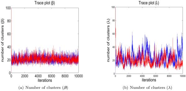
Trace plots of number of clusters for the regression coefficients and the precisions when fitting the gene expression data.

There were six large clusters for β with size more than 50. Those clusters included 897 genes. The average gene expressions for each one of the six clusters are shown in Figure 8(a). The y-axis indicates the average gene expressions, and the x-axis indicates the treatments. Each cluster shows its unique profile. We found one cluster of 18 genes with all regression coefficients equal to zero (Figure 8(b)).

Figure 8.

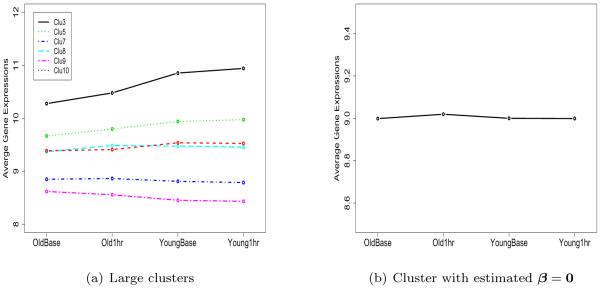
Average expression profiles for (a) six large clusters; (b) cluster with estimated β = 0.

For hypothesis testing, we ranked genes by calculating posterior probabilities for the genes least supportive of the null hypothesis, H_0,g : β_1,g = β_2,g = β_3,g = β_4,g = 0. We listed the fifty genes that were least supportive of the hypothesis H_0,g. Figure 9 shows the heatmap of those fifty genes.

Figure 9.

Heatmap of the 50 top-ranked genes which are least supportive of the assertion that β₁ = β₂ = β₃ = β₄ = 0.

Finally, in order to identified genes following the second hypothesis of interest H_a,g : |β_1,g - β_3,g|= 0 &|β_2,g - β_4,g| > 0.1, we similarly identified the top fifty ranked genes. For this hypothesis, our approach clearly finds genes following the desired pattern, as shown in Figure 10.

Figure 10.

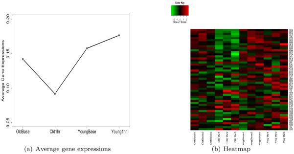
(a) Average gene expressions of the 50 top-ranked genes supportive of |β₁ − β₃| = 0 & |β₂ − β₄| > 0.1; (b) Heatmap of those genes

5 Discussion

We have proposed a semiparametric Bayesian method for random effects models in the context of multiple hypothesis testing. A key feature of the model is the use of a spiked centering distribution for the Dirichlet process prior. Dirichlet process mixture models naturally borrow information across similar observations through model-based clustering, gaining increased power for testing. This centering distribution in the DP allows the model to accommodate the estimation of sharp hypotheses. We have demonstrated via a simulation study that our method yields a lower proportion of false discoveries than other competitive methods. We have also presented an application to microarray data where our method readily infers posterior probabilities of genes being Differentially expressed.

One issue with our model is that the results are not necessarily invariant to the choice of the reference treatment. Consider, for example, the gene expression analysis of Section 4.2 in which we used the group (Old, Baseline) as the reference group. To investigate robustness, we reanalyzed the data using (Young, Baseline) as the reference group. We found that the rankings between two results are very close to each other (Spearman's correlation = 0.9937762, Figure 11).

Figure 11.

Scatter plot of rankings of genes resulting from using two reference treatments

Finally, as we mentioned in the Section 2.1, our current model can easily accommodate covariates by placing them in the X matrix. Such covariates might include, for example, demographic variables regarding the subject or environmental conditions (e.g., temperature in the lab) that affect each array measurement. Adjusting for such covariates has the potential to increase the statistical power of the tests.

Table 2.

Among the 50 most likely differentially expresed objects, the number in common among the pairwise intersection of the samples identified under the ten hyperparameter settings.

	(i)	(ii)	(iii)	(iv)	(v)	(vi)	(vii)	(viii)	(ix)
MOM (both)	41	37	41	38	39	41	39	39	42
(i)		42	45	45	45	42	45	43	46
(ii)			43	44	43	42	44	42	43
(iii)				45	45	43	45	46	46
(iv)					44	40	47	42	44
(v)						45	44	44	45
(vi)							42	44	45
(vii)								45	44
(viii)									44

1 Appendix

1.1 Full Conditional for Precision

$$\begin{array}{cc}\hfill p(\tau \mid \mathbf{d},\beta ,\lambda )& \propto p\left(\tau \right)\prod _{S\in \xi }p({\beta }_S\mid \pi ,\tau )p({\mathbf{d}}_S\mid {\beta }_S,{\lambda }_S,\pi ,\tau )\hfill \\ \hfill & =\left\{\prod _{t=1}^{T}p\left({\tau }_t\right)\right\}\left\{\prod _{S\in {\zeta }_t}\prod _{t=1}^{T}p({\beta }_{\mathit{St}}\mid {\pi }_t,{\tau }_t)\right\}\hfill \\ \hfill & \propto \prod _{t=1}^{T}p\left({\tau }_t\right)\left\{\prod _{S\in {\zeta }_t}N({\beta }_{S_t}\mid m_t,{\tau }_t)\right\}\hfill \\ \hfill & \propto \prod _{t=1}^T{\tau }_t^{a_t+\mid {\zeta }_t\mid ∕2-1}\exp \left\{-{\tau }_t\left(\frac{1}{b_{\tau }}+\frac{1}{2}\sum _{S\in {\zeta }_t}{({\beta }_{S_t}-m_t)}^2\right)\right\}\hfill \end{array}$$

1.2 Full Conditional for new probability y_t = ρ_tr_π of Spike

Note: modified prior ρ_tr_π = p(β_t = 0) where r_π = a_π/(a_π + b_π), thus need a posterior ρ_t|rest ∝ p(β_t = 0|rest).

Set Y_t = r_πρ_t. Then the distribution of Y_t is

$$\begin{array}{cc}\hfill p\left(y_t\right)& =\frac{1}{B(a_{\rho },b_{\rho })}{\left(\frac{y_t}{r_{\pi }}\right)}^{a_{\rho }-1}{\left(1-\frac{y_t}{r_{\pi }}\right)}^{b_{\rho }-1}\frac{1}{r_{\pi }}\hfill \\ \hfill & =\frac{1}{B(a_{\rho },b_{\rho })}{\left(\frac{1}{r_{\pi }}\right)}^{a_{\rho }+b_{\rho }-1}{y}_t^{a_{\rho }-1}{(r_{\pi }-y_t)}^{b_{\rho }-1}.\hfill \end{array}$$

Now, we are drawing Y_t, not ρ_t from their conditional distributions: for t,

$$p(y_t\mid \text{rest})\propto p\left(y_t\right)y_t^{{\Sigma }_{S\in \xi }I({\beta }_{\mathit{St}}=0)}{(1-y_t)}^{{\Sigma }_{S\in \xi }I({\beta }_{\mathit{St}}\ne 0)},$$

which is not of known form of distribution. Once we draw samples of Y_t, then we will get ρ_t as Y_t/r_π. We used a grid-based inverse-cdf method. for sampling Y_t.

1.3 Full Conditional for Regression coefficients

$$\begin{array}{cc}\hfill & p({\beta }_{\mathit{St}}\mid {\lambda }_S,{\mathit{d}}_S,y_t,{\beta }_{S(-t)})\propto p({\beta }_{\mathit{St}}\mid y_t)\prod _{g\in S}p({\mathit{d}}_g\mid {\beta }_{\mathit{St}},{\beta }_{S(-1)},{\lambda }_S)\hfill \\ \hfill =& y_t{\delta }_0\left({\beta }_{\mathit{St}}\right)\prod _{g\in S}p({\mathit{d}}_g\mid {\beta }_{\mathit{St}},{\beta }_{S(-t)},{\lambda }_S)+(1-y_t)N({\beta }_{\mathit{St}}\mid m_t,{\tau }_t)\prod _{g\in S}p({\mathit{d}}_g,{\beta }_{\mathit{St}}{\beta }_{S(-t)},{\lambda }_S)\hfill \end{array}$$

The first part is obvious. Look at the second part. Set x_t = (X_1t, …, X_Kt)^T, X(−t) = (x₁, ⋯ . x_(t−1), x_(t+1), ⋯ , x_T), and β_S(−t) = (β_S1, ⋯ , β_S(t−1), β_S(t+1), ⋯ , β_ST)^T

The second part is proportional to:

$$\begin{array}{cc}\hfill \exp \left\{-\frac{1}{2}{\tau }_t{({\beta }_{\mathit{St}}-m_t)}^2\right\}\times \exp & \left[-\frac{1}{2}\left\{\sum _{g\in S}{\mathit{D}}_g^T{\mathit{Q}}_g{\mathit{D}}_g\right\}\right]\hfill \\ \hfill & \text{where}{\mathit{D}}_g={\mathit{d}}_g-{\mathit{x}}_t{\beta }_{\mathit{St}}-\mathit{X}(-t){\beta }_{S(-t)}-{\mathit{E}}_g^{-1}{\mathit{f}}_g\hfill \end{array}$$

$$\propto \exp \left\{-\frac{1}{2}({\tau }_t{\beta }_{\mathit{St}}^2-2{\tau }_t{m}_t{\beta }_{\mathit{St}})\right\}\exp \left\{-\frac{1}{2}\sum _{g\in S}{({\mathit{x}}_t{\beta }_{\mathit{St}}-{\mathit{A}}_g)}^T{\mathit{Q}}_g({\mathit{x}}_t{\beta }_{\mathit{St}}-{\mathit{A}}_g)\right\}$$

$$\propto \exp \left[-\frac{1}{2}\left\{{\beta }_{\mathit{St}}^2({\tau }_t+\sum _{g\in S}{\mathit{x}}_t^T{\mathit{Q}}_g{\mathit{x}}_t)-2{\beta }_{\mathit{St}}(m_t{\tau }_t+\sum _{g\in S}{\mathit{x}}_t^T{\mathit{Q}}_g{\mathit{A}}_g)\right\}\right].$$

Therefore, for each t,

$${\beta }_{\mathit{St}}\mid \cdot =\{\begin{array}{cc}0\hfill & \text{with probability}{\pi }_{\mathit{st}}\hfill \\ ~N\left(\frac{m_t{\tau }_t+{\Sigma }_{g\in S}{\mathit{x}}_t^T{\mathit{Q}}_g{\mathit{A}}_g}{{\tau }_t+{\Sigma }_{g\in S}{\mathit{x}}_t^T{\mathit{Q}}_g{\mathit{x}}_t},{\tau }_t+{\Sigma }_{g\in S}{\mathit{x}}_t^T{\mathit{Q}}_g{\mathit{x}}_t\right)\hfill & \text{with probability}1-{\pi }_{\mathit{st}}.\hfill \end{array}\phantom{\}}$$

References

- Antoniak CE. Mixtures of Dirichlet Processes With Applications to Bayesian Nonparametric Problems. The Annals of Statistics. 1974;2:1152–1174. 710. [Google Scholar]
- Baldi P, Long AD. A Bayesian framework for the analysis of microarray expression data: regularized t-test and statistical inferences of gene changes. Bioinformatrics. 2001;17:509–519. doi: 10.1093/bioinformatics/17.6.509. 708. [DOI] [PubMed] [Google Scholar]
- Benjamini Y, Hochberg Y. Controlling the False Discovery Rate: A Practical and Powerful Approach to Multiple Testing. (Series B: Methodological).Journal of the Royal Statistical Society. 1995;57:289–300. 708. [Google Scholar]
- Berry DA, Hochberg Y. Bayesian Perspectives on Multiple Comparisons. Journal of Statistical Planning and Inference. 1999;82:215–227. 708. [Google Scholar]
- Binder DA. Bayesian Cluster Analysis. Biometrika. 1978;65:31–38. 715. [Google Scholar]
- Brown P, Vannucci M, Fearn T. Multivariate Bayesian variable selection and prediction. J. R. Statist. Soc. B. 1998;60:627–41. 711. [Google Scholar]
- Cai B, Dunson D. Technical report. Department of Statistical Science; Duke University: 2007. Variable selection in nonparametric random effects models. 709. [Google Scholar]
- Dahl DB. Model-Based Clustering for Expression Data via a Dirichlet Process Mixture Model. In: Do K-A, Müller P, Vannucci M, editors. Bayesian Inference for Gene Expression and Proteomics. Cambridge University Press; 2006. pp. 201–218. 715. [Google Scholar]
- Dahl DB, Mo Q, Vannucci M. Simultaneous Inference for Multiple Testing and Clustering via a Dirichlet Process Mixture Model. Statistical Modelling: An International Journal. 2008;8:23–39. 708, 709, 711, 713, 719, 720. [Google Scholar]
- Dahl DB, Newton MA. Multiple Hypothesis Testing by Clustering Treatment Effects. Journal of the American Statistical Association. 2007;102(478):517–526. 708, 711. [Google Scholar]
- Do K-A, Müller P, Tang F. A Bayesian mixture model for differential gene expression. Journal of the Royal Statistical Society: Series C (Applied Statistics) 2005;54(3):627–644. 708. [Google Scholar]
- Dudoit S, Gibert HN, van der Laan MJ. Resampling-Based Empirical Bayes Multiple Testing Procedures for Controlling Generalized Tail Probability and Expected Value Error Rates: Focus on the False Discovery Rate and Simulation Study. Biometrical Journal. 2008;50:716–744. doi: 10.1002/bimj.200710473. 719. [DOI] [PMC free article] [PubMed] [Google Scholar]
- Dudoit S, Shaffer JP, Boldrick JC. Multiple Hypothesis Testing in Microarray Experiments. Statistical Science. 2003;18(1):71–103. 708. [Google Scholar]
- Dudoit S, Yang YH, Callow MJ, Speed TP. Statistical methods for identifying differentially expressed genes in replicated cDNA microarray experiments. Statistica Sinica. 2002;12(1):111–139. 708. [Google Scholar]
- Dunson DB, Herring AH, Engel SA. Bayesian Selection and Clustering of Polymorphisms in Functionally-Related gene. Journal of the American Statistical Association. 2008 in press. 709. [Google Scholar]
- Escobar MD, West M. Bayesian Density Estimation and Inference Using Mixtures. Journal of the American Statistical Association. 1995;90:577–588. 713. [Google Scholar]
- Genovese C, Wasserman L. Bayesian Statistics 7. Oxford University Press; 2003. Bayesian and Frequentist Multiple Testing; pp. 145–161. 717. [Google Scholar]
- George E, McCulloch R. Variable selection via Gibbs sampling. J. Am. Statist. Assoc. 1993;88:881–9. 711. [Google Scholar]
- Gopalan R, Berry DA. Bayesian Multiple Comparisons Using Dirichlet Process Priors. Journal of the American Statistical Association. 1998;93:1130–1139. 708. [Google Scholar]
- Hochberg Y. A Sharper Bonferroni Procedure for Multiple Tests of Significance. Biometrika. 1988;75:800–802. 708. [Google Scholar]
- Hommel G. A Stagewise Rejective Multiple Test Procedure Based on a Modified Bonferroni Test. Biometrika. 1988;75:383–386. 708. [Google Scholar]
- Irizarry R, Hobbs B, Collin F, Beazer-Barclay Y, Antonellis K, Scherf U, Speed T. Exploration, Normalization, and Summaries of High Density Oligonucleotide Array Probe Level Data. Biostatistics. 2003;4:249–264. doi: 10.1093/biostatistics/4.2.249. 724. [DOI] [PubMed] [Google Scholar]
- Lau JW, Green PJ. Bayesian model based clustering procedures. Journal of Computational and Graphical Statistics. 2007;16:526–558. 715. [Google Scholar]
- Lucas J, Carvalho C, Wang Q, Bild A, Nevins JR, Mike W. Sparse Statistical Modelling in Gene Expression Genomics. In: Do K-A, Müller P, Vannucci M, editors. Bayesian Inference for Gene Expression and Proteomics. Cambridge University Press; 2006. pp. 155–174. 711. [Google Scholar]
- MacLehose RF, Dunson DB, Herring AH, Hoppin JA. Bayesian methods for highly correlated exposure data. Epidemiology. 2007;18(2):199–207. doi: 10.1097/01.ede.0000256320.30737.c0. 708, 709. [DOI] [PubMed] [Google Scholar]
- Medvedovic M, Sivaganesan S. Bayesian Infinite Mixture Model Based Clustering of Gene Expression Profiles. Bioinformatrics. 2002;18:1194–1206. doi: 10.1093/bioinformatics/18.9.1194. 715. [DOI] [PubMed] [Google Scholar]
- Müller P, Parmigiani G, Robert C, Rousseau J. Optimal Sample Size for Multiple Testing: The case of Gene Expression Microarrays. Journal of the American Statistical Association. 2004;99:990–1001. 717. [Google Scholar]
- Neal RM. Markov Chain Sampling Methods for Dirichlet Process Mixture Models. Journal of Computational and Graphical Statistics. 2000;9:249–265. 714. [Google Scholar]
- Newton M, Kendziorski C, Richmond C, Blattner F, Tsui K. On differential variability of expression ratios: Improving statistical inference about gene expression changes from microarray data. Journal of Computational Biology. 2001;8:37–52. doi: 10.1089/106652701300099074. 708. [DOI] [PubMed] [Google Scholar]
- Newton MA, Noueiry A, Sarkar D, Ahlquist P. Detecting differential gene expression with a semiparametric hierarchical mixture method. Biostatistics. 2004;5:155–176. doi: 10.1093/biostatistics/5.2.155. 708, 719. [DOI] [PubMed] [Google Scholar]
- Scott JG, Berger JO. An Exploration of Aspects of Bayesian Multiple Testing. Journal of Statistical Planning and Inference. 2006;136:2144–2162. 708. [Google Scholar]
- Smyth GK. Linear models and empirical Bayes methods for assessing differential expression in microarray experiments. Statistical Applications in Genetics and Molecular Biology. 2004;3(No. 1) doi: 10.2202/1544-6115.1027. Article 3. 709, 719. [DOI] [PubMed] [Google Scholar]
- Storey J. The optimal discovery procedure: A new approach to simultaneous significance testing. (Series B).Journal of the Royal Statistical Society. 2007;69:347–368. 708. [Google Scholar]
- Storey J, Dai JY, Leek JT. The optimal discovery procedure for large-scale significance testing, with applications to comparative microarray experiments. Biostatistics. 2007;8:414–432. doi: 10.1093/biostatistics/kxl019. 708. [DOI] [PubMed] [Google Scholar]
- Storey JD. A Direct Approach to False Discovery Rates. (Series B: Statistical Methodology).Journal of the Royal Statistical Society. 2002;64(3):479–498. 708. [Google Scholar]
- Storey JD. The Positive False Discovery Rate: A Bayesian Interpretation and the q-value. The Annals of Statistics. 2003;31(6):2013–2035. 708. [Google Scholar]
- Storey JD, Taylor JE, Siegmund D. Strong Control, Conservative Point Estimation and Simultaneous Conservative Consistency of False Discovery Rates: a Unified Approach. (Series B: Statistical Methodology).Journal of the Royal Statistical Society. 2004;66(1):187–205. 708. [Google Scholar]
- Tibshirani R, Wasserman L. Technical Report 839. Department of Statistics; Carnegie Mellon University: 2006. Correlation-sharing for Detection of Differential Gene Expression. 708. [Google Scholar]
- Westfall PH, Wolfinger RD. Multiple Tests with Discrete Distributions. The American Statistician. 1997;51:3–8. 708. [Google Scholar]
- Westfall PH, Young SS. Resampling-based Multiple Testing: Examples and Methods for P-value Adjustment. John Wiley & Sons; 1993. 708. [Google Scholar]
- Yuan M, Kendziorski C. A Unified Approach for Simultaneous Gene Clustering and Differential Expression Identification. Biometrics. 2006;62:1089–1098. doi: 10.1111/j.1541-0420.2006.00611.x. 708. [DOI] [PubMed] [Google Scholar]