

Abstract
Tagged Magnetic Resonance Imaging (tagged MRI or tMRI) provides a means of directly and noninvasively displaying the internal motion of the myocardium. Reconstruction of the motion field is needed to quantify important clinical information, e.g., the myocardial strain, and detect regional heart functional loss. In this paper, we present a three-step method for this task. First, we use a Gabor filter bank to detect and locate tag intersections in the image frames, based on local phase analysis. Next, we use an improved version of the Robust Point Matching (RPM) method to sparsely track the motion of the myocardium, by establishing a transformation function and a one-to-one correspondence between grid tag intersections in different image frames. In particular, the RPM helps to minimize the impact on the motion tracking result of: 1) through-plane motion, and 2) relatively large deformation and/or relatively small tag spacing. In the final step, a meshless deformable model is initialized using the transformation function computed by RPM. The model refines the motion tracking and generates a dense displacement map, by deforming under the influence of image information, and is constrained by the displacement magnitude to retain its geometric structure. The 2D displacement maps in short and long axis image planes can be combined to drive a 3D deformable model, using the Moving Least Square method, constrained by the minimization of the residual error at tag intersections. The method has been tested on a numerical phantom, as well as on in vivo heart data from normal volunteers and heart disease patients. The experimental results show that the new method has a good performance on both synthetic and real data. Furthermore, the method has been used in an initial clinical study to assess the differences in myocardial strain distributions between heart disease (left ventricular hypertrophy) patients and the normal control group. The final results show that the proposed method is capable of separating patients from healthy individuals. In addition, the method detects and makes possible quantification of local abnormalities in the myocardium strain distribution, which is critical for quantitative analysis of patients’ clinical conditions. This motion tracking approach can improve the throughput and reliability of quantitative strain analysis of heart disease patients, and has the potential for further clinical applications.
Index Terms: Tagged MRI, Motion Tracking, Gabor Filter, RPM, Deformable Model, Strain
I. Introduction
Magnetic resonance imaging (MRI) has become one of the most effective means for the delineation of cardiac anatomic structures, as well as the extraction in vivo of physiological functional information. Clinically important information, such as motion, blood flow, and perfusion in the tissue, can be encoded as changes in pixel phase or intensity, and can be augmented using contrast agent enhancement during MRI scans. Recent developments in cardiac imaging with computed tomography (CT) have succeeded in generating 3D images of heart with higher spatial resolution and more detailed depiction of anatomic structures. However, the relatively low temporal resolution of CT and its inability to encode physiological information have limited the use of this modality mostly to the static reconstruction of the heart. In particular, CT is inaccurate at reconstructing and/or quantifying regional myocardial motion, because of the lack of information about the motion within the myocardium other than the motion at the epi- and endo- myocardial surfaces. Therefore, this image modality fails to provide some information that could potentially be useful in assessing patients with local cardiac functional loss or disorder, such as due to myocardial infarction and ischemia.
MRI is generally considered to be the current gold standard method for evaluating cardiac function. Among the MRI-based techniques, magnetization-tagged MRI is one of the earliest and still arguably the most efficient means to directly and non-invasively display the motion of the myocardium. Tagged regions are visible as darker stripes in tagged MR images. They deform as the underlying myocardium [1] [2] contracts periodically during the cardiac cycle. The advantage of tagged MRI over other imaging techniques is the direct and explicit reflection of the interior myocardial motion through the tags, which enables the qualitative and quantitative evaluation of the regional heart function, and the detection of regional heart function abnormalities.
Several image processing and analysis methods have been proposed for use with tagged MRI, but currently the most popular one is the automatic Harmonic Phase (HARP) method [3]. HARP is essentially a phase analysis of a single-sideband demodulation of the tags, carried out in the Fourier domain. Tag locations in the spatial domain are derived based on the inverse Fourier transform of one or two corresponding harmonic peaks of the image signal in the Fourier domain. Note that an assumption that HARP uses here is that the tag spacing and orientation in the current frame are approximately uniform (as illustrated by using only one harmonic peak to calculate the phase relative to the tag pattern at every pixel in the original image), which conflicts with the fact that local variations exist in tag spacing and orientation distributions at different frames during the cardiac cycle, due to the cardiac motion. This theoretic imperfection can lead to errors in the HARP output, such as bifurcations in the recovered tag map, which also deteriorates at boundaries, and in regions with large deformations or rotations.
Gabor filters [4] provide an alternative solution for automated tagged MRI analysis. They have some formal relationship to, but are distinct from, the HARP method. Gabor filters are sinusoidally modulated Gaussians, which can be convolved with an image to extract the local periodic “stripe” content; this convolution can be conveniently carried out in the Fourier domain. They are natural matches to different tag patterns in the spatial domain, as they can track the local variation of tag spacing and orientation by changing their parameters accordingly. The HARP method can be treated as a special case of Gabor filters, whose parameters are fixed despite the local variation in tagging. Some typical HARP errors, such as the false bifurcations, can be avoided or reduced by Gabor-based methods, as introduced in [5]. In [5] a bank of Gabor filters was used, with different parameters corresponding to different tag spacing and orientation, and the optimal ones to use for local phase estimation were chosen pixel-by-pixel. The displacement and the cardiac strain were then calculated, based on a refined phase map that incorporated the effects of local variation in tag spacing and orientation.
Both the HARP and Gabor filters are based on frequency domain analysis, and they share some common shortcomings for cardiac motion tracking. For example, both methods require an unwrapping step, which by itself is an error prone process, to convert the phase map into the displacement maps. Some other tag tracking methods, such as the use of deformable models [14, 18, 19, 24, 25] and spline models [6, 9, 10, 21], work in the image domain and produce the displacement map directly. These image-based methods use parameterized deformable models to converge the model to fit to the changing locations of the tag lines, under the influence of the image gradient. One major disadvantage of these methods is their nature of being driven by local features, which may lead to a mismatch between models and tag lines. Two of the most common scenarios of mismatch take place when: 1) the through-plane motion of the curved heart wall causes sudden disappearance or appearance of tags in 2D images close to the myocardial boundaries; and 2) as the heart contracts, tag spacing decreases enough to cause the local gradient-driven model to “jump” to the “wrong” tag and generate a mismatch. In addition, image-based methods are more sensitive to image noise.
By combining these approaches, using the frequency domain analysis and the image domain analysis together, we can improve the motion tracking performance. We present in this paper a motion tracking framework that integrates those two kinds of analysis, such that one helps to improve the performance of the other, and vice versa. The motion tracking starts with a Gabor filter-based phase analysis. We then use phase maps to find the locations of tag intersections at different times during the cardiac cycle. We track the motion of tag intersections between frames using the Robust Point Matching (RPM) method. Finally, we use an implicit deformable model to reconstruct the dense displacement map between two image frames as we register the segmented heart regions in those images, using the displacement magnitude as a constraint.
RPM [7] is a computer vision technique that was developed to find the correspondence between two sets of points. It has been widely implemented to solve rigid and nonrigid registration problems [7, 8, 26]. By using a simulated annealing scheme [8] and an extended correspondence matrix, it finds the correspondence between two point sets before and after large deformation and/or with different numbers of elements. However, special modifications and improvements have to be made to the original form of RPM in order to retain a consistent and robust performance in tracking the motion of tag intersections.
Traditional deformable models have been widely used for 2D and 3D cardiac motion reconstructions from tagged MRI, such as by Park et al. [4, 5, 6, 11, 17]. However, the performance of explicitly deformable models driven by Finite Element Methods (FEM) and splines can be affected by local noise, and they may generate singularities in the displacement map. For instance, one local noise region may attract two nearby spline models and cause them to collide, which will be reflected in the displacement map as a singularity point. One way to overcome the mismatch problem is to use more spatial and temporal constraints. However, this means a more complicated model structure and a longer computational time for the model to converge. Therefore, a better solution is to use the implicit form of the deformable model, embedded with spatial and temporal constraints, for better and more efficient convergence between the model and tags. In particular, the cardiac motion is a complicated combination of motions in 3D space. However, most currently available 3D deformable models of the heart are only illustrative, rather than ready for use in quantitative analysis, due to their complicated structures, lack of the capability of capturing motion fields with large variation, and high computation costs. This leads to the urgent need for a new 3D deformable model, with superior performance in object convergence and tracking, and capable of quantitative motion analysis. In our implementation, an implicit deformable model has been developed. The model reconstructs dense motion fields between two image frames by solving a registration problem and minimizing the residual motion errors at tag intersections. We propose in this paper a new deformation constraint, the overall displacement magnitude, to replace older ones, such as the separate displacement components. Efforts have been made to extend the model into 3D, and the preliminary results are very promising.
The rest of this paper is organized as follows: Section two introduces our new tag-based motion tracking method and its 3D extension. In section three we present experimental results on a numerical phantom, as well as on 2D and 3D in vivo heart data. We evaluate the method by comparing its results against the “ground truth” and other tag tracking methods and by measuring its timing performance. We provide a brief discussion and draw our conclusions in section four.
II. Method
A. Gabor Filter and Gabor Filter Bank
A Gabor filter can be simply expressed as a Gaussian multiplied by a complex sinusoid in the image domain, as shown below:
| (1) |
with (u0, v0) the center frequency, (x′, y′) = (x cosθ + y sinθ,−x sinθ + y cosθ) is (x, y) rotated by θ with respect to the x axis, and is a Gaussian filter with the spatial standard deviations σx, σy. The filter h(x, y) can be split into its real and imaginary components, hR and hI (even and odd functions, respectively):
| (2) |
| (3) |
and the Fourier transforms of the real (2) and imaginary (3) components of a Gabor filter are given by:
| (4) |
| (5) |
where G(u, v) = F{g(x, y)} and F{} denotes the Fourier transform. The final form of a 2D Gabor filter in the Fourier domain is
| (6) |
which is a pair of Gaussians at (u0, v0) and (−u0, −v0) in the Fourier domain. The inverse Fourier transform of the product of the filter and the Fourier transform (FT) of the image can be split into a phase map and a magnitude map in the image domain. The phase at a given material point is constant during the cardiac cycle, regardless of its location in the current frame: it is effectively a material property, just like the tag pattern from which it is derived. Phase is wrapped to be within the range [−π,π), so that there is a correspondence between tags and the phase map; pixels at the centerlines of tags have phase values of −π.
To accommodate local tag spacing and orientation changes, we multiply the FT of the image in the Fourier domain with a bank of Gabor filters with different parameter values, to generate multiple image domain phase maps corresponding to different tag spacing and orientation, and combine these maps to create the final phase map with local responses. In the Fourier domain, 2D Gabor filters can be defined using three global parameters: central frequency (u0, v0), orientation θ, and filter size σ, where u0 and v0 are the inverse of the corresponding horizontal and vertical tag spacing, respectively, θ corresponds directly to the tag orientation in the image domain, and σ is chosen proportional to the central frequency so that Gabor filter outputs are unified in magnitude. The Gabor filter bank is composed of filters with different tag spacing (e.g., with the interval of one pixel) in the image domain, and orientation angles θ =θini + n · Δθ, where n = 0,±1,±2,…, Δθ is the minimal angular difference, and θini = 0 for vertical tags, π/2 for horizontal tags. The magnitude of a Gabor filter’s output at a pixel is different for different parameter values, and is maximized when the parameter-set matches the local tag spacing and orientation. At each pixel, we choose the three Gabor filters with the highest output magnitude, and use the linear interpolation of their parameter values to construct a new Gabor filter. We multiply the filter with the FT of the image in the frequency domain. The new Gabor filter has parameters that are close to the local tag spacing and orientation, so that its phase response is a close estimation of the tag-based-phase at the pixel. We calculate the phase map pixel-by-pixel in this manner, so that local tag spacing and orientation are approximately optimally estimated.
Gabor filters have a good performance in displacement reconstruction, but several intrinsic defects of filter-based approaches prevent us from simply using the Gabor results directly. First, the Gabor filter may include irrelevant information (e.g., phase information outside the myocardium) when analyzing motion close to the myocardial boundary, which can cause its performance to deteriorate at myocardial boundaries. Second, the Gabor filter has difficulty capturing large deformations and abrupt variations in the displacement map, due to its smoothing nature. Third, the output of Gabor filters requires phase unwrapping, which is an error-prone process. And fourth, the Gabor filter only outputs an Eulerian displacement map at the current frame. Therefore, we have developed the following methods to improve the Lagrangian displacement map quality.
B. Robust Point Matching
To avoid the error-prone unwrapping process in displacement reconstruction algorithms like the HARP and the Gabor filter approaches, we find tag intersections at the local minima of the summation of wrapped phase maps for horizontal and vertical tags, as shown in Figure 2(c). This is a completely automatic process. The computed tag intersections will be used in the RPM, as described below.
Fig. 2.
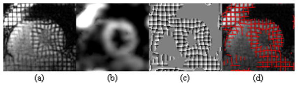
(a) A deformed grid tag image, (b) the magnitude output of Gabor filter bank, (c) 2D phase map generated by Gabor filter bank, and (d) tag lines (red) recovered from phase.
Suppose we are tracking the motion of tags from the ith (denoted as Ii) to the i + 1 th frame (denoted as Ii+1) in one image sequence. When neglecting the through-plane motion, tag intersections in these two frames can be viewed as two sets of material points with close correlation. Ideally, there is a one-to-one correspondence between tag intersections in two image frames, since they are unique in appearance and usually will not overlap with each other during the cardiac cycle. The motion-tracking task can then be reduced to the problem of finding this unknown correspondence between two sets of tag intersections. Let us denote tag intersections as P = {pj, j = 1,2,…M} and Q = {qk, k = 1,2,…N} for Ii and Ii+1, respectively. From Ii to Ii+1, the underlying motion field can be expressed as a non-rigid transformation function f. A point pj ∈ P in Ii is mapped to its new location f(pj) in Ii+1. The matching problem is equivalent to the minimization of the energy function EZ,f:
| (7) |
where Z = zjk is a binary correspondence matrix, its elements zjk ∈ {0,1} for j = 1,2,…M +1 and k = 1,2,…N + 1. The correspondence matrix is subject to the constraints for k = 1,2,…N and for j = 1,2,…M. The second term is a smoothness constraint that enforces the minimization of the second order derivatives of the transformation function. One problem caused by the through-plane motion of the curved heart wall is that tag intersections close to the myocardial boundary may move in or out of the image plane at different frames, which will cause those tag intersections to appear and disappear in different frames of the image sequence. These tag intersections are treated as unpaired outliers. In Z, the M + 1 row and the N + 1 column are dedicated to these outliers and the third term in equation (8) is a constraint that controls the number of outliers in the final correspondence matrix. ζ is the weight that controls the strength of the constraint: as ζ decreases, we allow less outliers in the final correspondence matrix. This way, when a tag intersection disappears (or appears) in the target image frame, it will be assumed to be an outlier, and will not contribute directly to the reconstruction of the displacement.
Because of the complexity of the heart motion, it can be hard to find the correspondence between P and Q using only a rigid transformation function and the traditional way of pairing points in different image frames based solely on their locations. To accommodate the need for nonrigid point matching, we use a deterministic annealing tracking scheme introduced in [15]. First, we replace Z in (7) with a fuzzy correspondence matrix Y, and rewrite the energy function in (7) as:
| (8) |
where still satisfies for k = 1,2,…N and for j = 1,2,…M with yjk ∈ [0,1]; T is a “temperature” parameter that can be adjusted during the tracking process.
The sum of the first two terms on the right hand side of Equation (8) is the “thin plate spline” (TPS) energy, which can be rewritten in the form:
| (9) |
where element qj′ in Q′ is defined by , d is the 3 by 3 affine transformation matrix, c is the M by 3 wrapping coefficient, and φ is the TPS kernel whose element φij = ||pi − pj||2 log||pi − pj||. Equation (9) can be solved using the QR decomposition [15], in which the coordinates of p are decomposed to enable the separation of the affine and non-affine transformations. Then we can compute the local deformation vector φc and the affine transformation matrix d, as described in [7].
Note that the energy term controls the minimization of the energy function in (8), through equation (9). The temperature parameter T is higher at the start of the tracking process, so that the energy function initially favors fuzzy correspondence matrix Y to maintain its convexity, which is reflected by the definition of Q in (9). As T gradually decreases to zero, the effect of the energy term gets weaker, so as to allow a binary solution of Y, and the formulation of Q changes correspondingly.
As noted above, the Gabor output alone of the tag intersection locations may not be accurate, especially when there is large deformation. Therefore, we use the fact that the tag intersections are local minima of image intensities and add another energy term:
| (10) |
to the right side of equation (8), where λimg is the weight for image intensity. This energy term is integrated into the energy minimization by replacing Q in (9) with Q′ = Q − t∇I(Q), where ∇ is the gradient operator, and t is the step size.
The myocardium around the LV is an approximately symmetric ring structure in short axis images, and point flipping can take place when using the traditional RPM, with a relatively high likelihood and frequency. To prevent flipping in the final transformation function, we set an upper limit for displacement magnitude, s = max(min(pj − qk)), for the local deformation vector elements. This will also prevent flipping in the affine transformation since it does not allow dramatic changes in point distributions in one iteration of point matching.
This new form of RPM generates a smooth transformation function f: R2 → R2 that approximately captures the displacement at tag intersections and estimates the displacement in the rest of image by minimizing the combination of the TPS energy and the image intensity energy. It is different from the original form of the RPM, and has an improved performance as part of the new motion tracking framework.
C. Deformable Model
RPM uses the locations of tag intersections but neglects the information available along the rest of the tags. To reconstruct a dense 2D displacement field and make full use of the tag information, we use deformable models to further refine the result of RPM. Deformable models of the x and y displacements are initialized using the transformation function generated via RPM. To reduce structural errors, such as singularities, and to make the model evolution more stable, we have developed an implicit deformable model.
Assume that the transformation function is defined in the image plane as f(x, y) = (u(x, y), v(x, y)), where u and v are the x (horizontal) and y (vertical) component of the transformation, respectively; we can redefine u and v as 3D surfaces u(x, y) = z and v(x, y) = z, where x and y are within the 2D image domain, and z ∈ R. The imaged 2D motion can be reconstructed as these 3D surfaces of u and v evolve under the influences of the image information and a smoothness constraint. The combined energy on these two deformable surfaces can be defined as:
| (11) |
Here,
| (12) |
where and are the x and y displacement at tag intersection k calculated using the TPS energy minimization.
Φ2 is determined by the image intensity gradient and has the following form:
| (13) |
where G is an Gaussian operator, I is the target image frame, Ω is the set of pixels along the tag line and within the myocardium, and (x′, y′) = (x + u, y + v) is the deformed location of tag point (x, y).
Φ3 is the phase constraint, which takes the form:
| (14) |
where Px and Py are unwrapped phase maps for the template image derived from the horizontal and vertical tags, respectively, and Px′ and Py′ are unwrapped phase maps for the target image derived from the horizontal and vertical tags, respectively.
Φ4 is the smoothness constraint. Displacements in the x and y directions are reflected separately by the motion of horizontal and vertical tags. In previous work, smoothness of displacements in different directions (u and v) were generally treated separately [6] because of this. However, we have found that the magnitude of the overall displacement is a better smoothness constraint. First, the smoothness of the magnitude of the displacement vector is physically meaningful. Neighboring material points in the myocardium deform with similar magnitude. Second, the smoothness of the overall displacement magnitude is easier to control, as illustrated in Figure 3. The magnitude map is smoother, with smaller range and less variation, while the x and y displacements can change much more rapidly: usually there will be at least two peaks and two saddles in the myocardium for each component of the displacement. And third, by constraining the model smoothness with the overall displacement magnitude, x and y displacements are more tightly bonded with each other. If in a certain part of the heart displacement in one direction is sparsely sampled (which may cause over-smoothing), the other displacement component will serve as a complementary smoothness constraint for the evolution of both deformable surfaces of the displacement.
Fig. 3.

First row from left to right: 3D map of the x component of the displacement, the y component of the displacement, and the magnitude of the corresponding overall displacement. The altitude of 3D surfaces corresponds to the magnitude of the variables. Second row: 2D color plots of the x displacement, y displacement, and the overall magnitude of the displacement. Notice in both cases, the magnitude of the overall displacement is more homogeneous and easier to use as a constraint.
Defining the displacement magnitude field as , we can define Φ4 as
| (15) |
where m″ and m‴′ are the second and fourth order derivatives of the magnitude field, respectively. We assume the 3D surface of m sustains the thin membrane energy. Therefore the reconstruction of the dense displacement field is equivalent to the generation of two smooth 3D deformable surfaces corresponding to u and v, as shown in Figure 4. For simplicity, these two surfaces are considered to only deform perpendicular to the image plane, and the motion at each point on the surface is defined by the Lagrange equation:
| (16) |
| (17) |
where fu and fv are external forces corresponding to u and v, respectively. Both forces are combinations of forces derived from Φ1, Φ2, and Φ3, such that:
| (18) |
| (19) |
where f1u and f1v are linear combinations of and at the four tag intersections closest to the current image pixel, respectively. f2u and f2v are derived from the x and y components of the local image intensity gradient at tag intersections, and f3u and f3v are derived from the x and y components of the phase difference within the myocardial mask. The derivation procedure is relatively intuitive.
Fig. 4.

(a) The undeformed numerical phantom, (b) the deformed phantom, (c) magnitude of in-plane displacement within the numerical phantom (ground truth), and the displacement magnitude maps generated (d) by the new method, (e) by HARP, and (f) by using Gabor filters output directly.
K in equations (16) and (17) is a stiffness matrix, as defined in [14]. It is derived from Φ4 and only affects the overall displacement magnitude. In (16) and (17), the internal system constraint derived from K is decomposed into components corresponding to u and v displacements, in order to calculate the evolution of u and v.
The pseudo code for the evolution of u and v is shown as follows:
| Deformable Model Pseudo-Code: |
| Initialize α1, α2, α3, and α4. |
| Begin A: Model Evolution. |
| Begin B: External Force Update. |
| Step 1: Update fu and fv; |
| Step 2: Update u and v using u′ = u + fu·Timestep, v′ = v + fv·Timestep |
| End B |
| Update m as |
| Begin C: Internal Feedback. |
| Step 1: Compute internal force fint = −Km′ |
| Step 2: Decompose fint into and |
| Step 3: Update u and v using u = u′+uint, v = v′+vint |
| End C |
| Evaluate the change of u and v. If small End A |
| End A |
D. 3D Extension
We extended our motion-tracking method into 3D, using a meshless deformable model. The meshless deformable model is a new form of deformable model with flexible geometric structure and less computational expense (sees reference [12, 13, 16, 20]). For 3D motion tracking, a group of (usually more than 5 slices) short axis (SA) and long axis (LA) cardiac images are acquired, using the tagged MRI technique, as shown in Figure 5. The SA images sampled the left ventricle (LV) at different levels from base to apex, and the LA images sampled the heart in three different views with approximately 60 degrees angles in between them, corresponding to the two-chamber, three-chamber, and four-chamber views of the heart. Eulerian displacements in the LA images are first computed to find the longitudinal motion during the cardiac cycle. Longitudinal motions at the intersections of LA and SA image planes are then interpolated within each of the SA image planes, to generate a map of through-plane motion in the 2D image plane at the current frame. The longitudinal motion and the in-plane motion calculated using the deformable model generate motion samplings in 3D. A geometrical mesh of the heart developed in [23] is used to accommodate the 3D motion at the sampled points as the driving forces for its deformation in 3D.
Fig. 5.

RPM tracking results for SA (first row) and LA (second row) tagged MRI. In the left column are original images with the initial locations of tag intersections highlighted using red dots. In the right column are deformed images. Red circles indicate the initial locations of tag intersections, and yellow dots indicate the current locations of tag intersections. Yellow arrows are used to connect correlated tag intersections. Notice that by having the one-to-one correspondence between tag intersections, the non-rigid transformation between two image frames is implicitly displayed. Also notice that the deformation between two images is large enough that it is impossible to reliably match two tag intersections by their locations alone. Notice in the right column images, there are yellow arrows that start without red circles (which means these intersections are not in the undeformed image, i.e., these are outlier intersections that move into the image plane), as well as red circles that do not have yellow arrows attached (outlier intersections that move out of the image plane in the current frame).
Given the 3D motion at sampled points q in the 2D image planes, we can calculate their initial locations p at the first (undeformed) frame. Thus, the 3D non-rigid deformation can be expressed as:
| (20) |
where f(·) is the displacement function, which combines the global and local terms, M is the global rigid translation matrix, and T is the non-rigid deformation at sampled points. In a meshless deformation, the displacement at an arbitrary point j in 3D can be calculated by minimizing the energy:
| (21) |
where wij are weights of sample points pi at point j during the energy minimization, and fj(·) is the local displacement function at j. The weights wij are distance-based, so that sample points far away from j have less weight during the energy evolution, while motions at nearby sample points have larger impacts on the motion at j. The displacement fj(·) can be conveniently solved for by applying derivative operators on both sides of equation (21) and calculating for the global and local deformation separately, by replacing fj(·) with the right hand side of (20).
The quality of the 3D motion was evaluated by manually tracking the 2D in-plane motion and measuring the difference between the imaged 2D motion and the intersection of the reconstructed 3D motion on the same image plane. We show some preliminary 3D experimental results in section III.
III. Experiments
We begin with a summary of all the parameters that control the behavior of the motion tracking framework. During the generation of the phase map, three parameters are defined for each filter in the Gabor filter bank: central frequency (u0, v0), orientation θ and the filter size σ; there are 5 different central frequencies and 5 different orientations, which are combined to form a total of 25 filters in the Gabor filter bank. We empirically found that an angular difference Δθ of π/18, a central frequency difference one tenth of the original central frequency, and a filter size proportional to the center frequency best balance the performance and efficiency for most data sets. Smaller parameter variations may increase the computational time for phase maps, while larger steps may cause inaccurate estimations of local phases. In the RPM step, three parameters have the biggest impact on the final point matching outcome: the annealing temperature, T, the local deformation upper threshold, s, and the weight for outlier acceptance, ζ. To make the point matching process more adaptive, all three parameters are defined depending on the data sets to be matched. Denoting the set of distances between any pair of tag intersections in the source frame to be dp, the initial value of T is defined as a·mean(||dp||2), where a is a constant empirically assigned with the value of 0.01. The value of T decreases at a rate such that Ti+1 = Ti*0.93 during the annealing, and the matching process stops when T < 0.01. Denoting the distance between a source tag intersection and its closest match in the target point set in the current iteration to be dpq, we define s = 0.5·mean(||dpq||). We set the upper threshold for the acceptance of outliers during point matching to be 5% of the size of the target set of tag intersections. Finally, in the deformable model, the weights for the four terms in the energy function in equation 11 have the relative ratios α1: α2: α3: α4 = 0.4: 0.1: 0.1: 0.4.
We tested our method on a numerical phantom. An annulus is overlaid with grid tags. It deforms following an underlying 2D displacement field similar to that seen in vivo, which we used as the “ground truth” in the validation of our method. We also compared the displacement maps generated by our method against those generated using the HARP method or directly from Gabor filters. In Figure 4, displacement magnitude maps for the end systole (ES) frame generated using our new method, from HARP, and directly from Gabor filters, are displayed together. The map generated using the new method shows higher accuracy and is smoother than the other two. In Table 1 we summarize the RMS errors of these three methods during the cardiac cycle and their ratio to the average displacement. By the standard of RMS error, our new motion tracking method outperforms both HARP and direct Gabor filter displacement mapping for the phantom data. We noted that our method tracks the cardiac motion better, particularly when the magnitude of the motion is large (comparable to the initial tag spacing). Another advantage our new method has over the previously developed phase-based displacement computational tools like HARP is that the error is not accumulated during the cardiac cycle. We notice that in the initial frames, the RMS error of our method is equal to or slight larger than those of the HARP and Gabor filters. However, as the heart starts contracting during systole, the errors of the HARP and Gabor accumulate, since the displacement in one frame is calculated based on previous frames. Even after the ES, when the myocardium relaxes and the displacement decreases, the error of these phase based methods keeps increasing, as opposed to our method.
TABLE I.
| Frame | 1 | 2 | 3 | 4 | 5 | 6 | 7 | 8 | 9 | 10 |
|---|---|---|---|---|---|---|---|---|---|---|
| Mean Disp. | 0.0 | 1.1234 | 2.4574 | 4.0282 | 5.0850 | 5.6400 | 5.0902 | 4.0527 | 2.3180 | 0.9968 |
| RMS Error | 0.0 | 0.1491 | 0.1936 | 0.1921 | 0.2558 | 0.3570 | 0.3677 | 0.3505 | 0.2578 | 0.2029 |
| RMS Ratio (%) | NA | 13.27 | 7.88 | 4.77 | 5.03 | 6.33 | 7.22 | 8.65 | 11.12 | 20.36 |
| HARP Error | 0.0 | 0.1054 | 0.1655 | 0.2996 | 0.4899 | 0.7120 | 0.6171 | 0.5071 | 0.6309 | 0.8222 |
| HARP Ratio (%) | NA | 9.38 | 6.74 | 7.44 | 9.63 | 12.62 | 12.12 | 12.51 | 27.22 | 82.48 |
| Gabor Error | 0.0 | 0.0954 | 0.1978 | 0.3536 | 0.5644 | 0.7192 | 0.6091 | 0.4104 | 0.2402 | 0.3319 |
| Gabor Ratio (%) | NA | 8.49 | 8.05 | 8.78 | 11.10 | 12.75 | 11.97 | 10.13 | 10.36 | 33.29 |
Comparison of motion tracking of numerical phantom by the new motion tracking method against HARP and Gabor-based methods, measured by the RMS error with respect to the ground truth. The 2nd row is the actual mean displacement magnitude in the phantom at 10 time frames; the 3rd and 4th rows are the RMS error in displacement magnitude with the new motion tracking method and its ratio with respect to the ground truth, respectively; 5th and 6th rows: corresponding HARP results; and 7th and 8th rows: corresponding Gabor results.
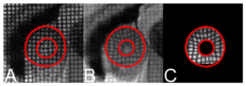
We also tested the performance of our method on in vivo heart data. Human imaging studies were performed under an Institutional Review Board-approved protocol. In Figure 5 we present representative point matching results of RPM for SA (upper row) and LA (lower row) tagged MRI. In both cases, tag intersections have been tracked accurately despite large and inhomogeneous motion. The automated tracking results have been evaluated by comparing them with manual tracking results of an expert, and the over 95% correlation indicates the strength of RPM.
We then tested the overall motion tracking performance of the new method. First, we tested the strength of the motion tracking method by reconstructing a deformed image given the undeformed image, and the Lagrangian motion field obtained using our approach. The original image, the target image, and the reconstructed image are shown side by side in Figure 6. The correlation coefficient between the segmented regions in the target image and the reconstructed image is 0.8065, which shows a high level of similarity between them, allowing for tag fading in the target image. The motion tracking results of a normal volunteer and a patient with hypertrophic cardiomyopathy (HCM) are shown in Figure 7 (above and below, respectively). The 2D displacement fields in two SA images are first displayed using the tag mesh regenerated using the displacement field. Then we show the reconstructed 2D displacement field, first in its separate x and y components, and then in its magnitude. Tags reconstructed using the displacement information matched well with the image information. We quantitatively evaluated the absolute value of the distance between the reconstructed tags and the manually tracked tags; the results for 6 healthy volunteers and 11 LVH patients are shown in the last column in Table 2. Also notice the difference between displacement maps of the normal subject and the patient, especially between the displacement magnitude maps, in which a large regional variation can be observed in the patient’s heart.
Fig. 6.
(a) The original ED image, with the LV myocardium delineated by red lines; (b) the deformed target image at ES; and (c) the ES image reconstructed using the displacement field and the ED image.
Fig. 7.
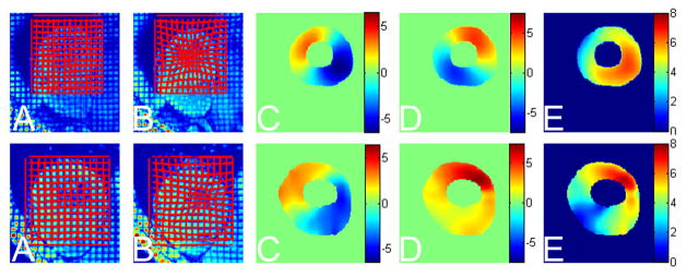
Top row: tag tracking in the myocardium of a healthy volunteer. Bottom row: tag tracking in the myocardium of a patient with asymmetric hypertrophic cardiomyopathy (HCM). In each group: A) are undeformed images overlaid with tag grids (red lines) generated by the displacement field (which is initially close to, but not necessarily, zero, due to the small deformation that may take place between the creation of tags and the acquisition of the first frame), B) are deformed images overlaid with tag grids reconstructed using the displacement field; C) and D) the x and y components of the Lagrangian displacement (so they are shown in the corresponding region of myocardium in the first frame) (notice that the normal heart has an approximately symmetric motion, while the patient’s heart moves more irregularly); and E) are the displacement magnitude maps. The normal heart has a more evenly and smoothly distributed displacement magnitude map, while the patient’s heart shows reduced contraction in most parts except for the upper right region. Same color ranges are used for images in the same column.
TABLE II.
| Group | CS Peak(%) | CS Time (%) | Absolute tag error (pixels) |
|---|---|---|---|
| Normal | −25.47 ± 7.52 | 33.29 ± 3.11 | 0.35 ± 0.07 |
| Patients | −14.42 ± 3.57 | 40.07 ± 4.31 | 0.29 ± 0.09 |
Summary of the circumferential strain (CS) and motion tracking performance in 11 LVH patients and 6 normal volunteers. The second column corresponds to the average and variance of peak values of the circumferential strain (in percentage); the third column corresponds to the average and variance of the time the circumferential strain reaches its peak (usually the end of systole), as a percentage of one cardiac cycle; and the fourth column corresponds to the average and variance of the difference of the automatic and manual tag tracking results.
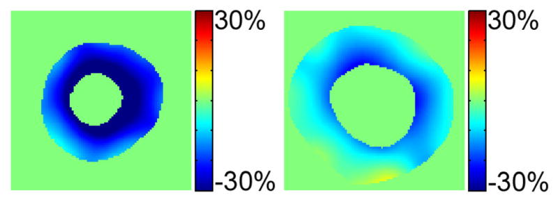
One potential clinical application of the proposed motion tracking method is for quantitative analysis of the myocardial strain, and in particular, to evaluate the local heart function as well as global heart function. In Figure 8, we display the in-plane myocardial strain maps at ES, derived from the motion tracking results for the healthy volunteer and the patient in Figure 7, respectively. The strain maps indicate heart functional differences, both globally and locally. Globally, the contraction in the normal heart produces higher strain (absolute value) than that of the patient’s heart. Locally, we notice that for the patient’s heart, a relatively small portion (in the 2 to 3 o’clock location) of the myocardium contracts normally while the rest of the heart contracts with less strain. Such information may be helpful in the diagnosis and treatment of heart disease. We also calculated the statistics of 17 different variables related to the circumferential strain distribution in the LVH patients and the normal controls, as shown in Table 3. The results show that these two groups have significant motion differences and can be readily separated from each other on the basis of the recovered motion variables. In Figure 9, more detailed SA circumferential strain maps at ES are shown for a normal volunteer and a LVH patient. Note that Figure 9 is generated using the magnitude smoothness term Φ4 while Figure 8 is generated without it, therefore displacement maps in Figure 9 are of higher smoothness and yet retain the critical clinical information on strain distribution. We can observe a clear pattern of greater circumferential shortening near the endocardial surface, both for the volunteer and the patient, which is consistent with previous findings. In Figure 10, we compare the strain in the same numeric phantom, generated obtained using HARP, the Gabor filters, and our motion tracking framework, against the actual strain. The histogram of the strain magnitude shows that the new motion tracking framework produces the closest estimation of the actual strain. In Figure 11, the RMS errors in the strain maps are displayed in the form of box plot. The strain generated by the new method has a smaller average error and less variation.
Fig. 8.

Left: strain distribution in the healthy heart. Right: strain distribution in HCM patient’s heart. Notice that the strain maps are more uniform than the displacement maps; also notice that the magnitude of the circumferential strain in patient’s heart is unevenly distributed. The heart has decreased contraction in most parts, but still contracts normally in the upper right region.
TABLE III.
| Measure* | LVH | Normal | P Value |
|---|---|---|---|
| Eccms | −0.061 ± 0.03 | −0.152 ± 0.03 | <0.0001 |
| Eccp | −0.117 ± 0.05 | −0.251 ± 0.06 | <0.0001 |
| Edotpd | 0.582 ± 0.22 | 1.671 ± 0.57 | <0.0001 |
| Edotps | −0.625 ± 0.17 | −1.411 ± 0.28 | <0.0001 |
| TedotpdTd | 0.246 ± 0.12 | 0.171 ± 0.05 | <0.0001 |
| TedotpsTs | 0.448 ± 0.16 | 0.320 ± 0.11 | 0.0075 |
| TecchpdTd | 0.331 ± 0.11 | 0.217 ± 0.05 | 0.0175 |
| Tedotps | 155.6 ± 57.9 | 99.8 ± 32.5 | 0.0331 |
| Eccms/Eccp | 0.501 ± 0.13 | 0.610 ± 0.09 | 0.0564 |
| Eccmd/Eccp | 0.303 ± 0.16 | 0.141 ± 0.06 | 0.0765 |
| TecchpsTs | 0.492 ± 0.10 | 0.431 ± 0.05 | 0.0834 |
| Tecchpd | 535.1 ± 62.5 | 470.8 ± 43.2 | 0.1105 |
| Tedotpd | 474.9 ± 60.1 | 437.4 ± 44.9 | 0.1348 |
| Tecchps | 171.2 ± 40.6 | 136.7 ± 19.8 | 0.1578 |
| Tcycle | 935.1 ± 101.4 | 1010.6 ± 74.5 | 0.2735 |
| Ts | 344.8 ± 55.1 | 326.3 ± 41.1 | 0.4338 |
| Eccmd | −0.030 ± 0.01 | −0.039 ± 0.01 | 0.9799 |
where
| Eccms | Ecc at mid systole |
| Eccp | Peak (absolute) Ecc |
| Edotpd | Peak (absolute) diastolic Edot* |
| Edotps | Peak (absolute) systolic Edot |
| TedotpdTd | Fraction of diastole of time of Edotpd |
| TedotpsTs | Fraction of systole of time of Edotps |
| TecchpdTd | Fraction of diastole of time of half of Eccp |
| Tedotps | Time of peak (absolute) systolic Edot |
| Eccms/Eccp | Fraction of Eccp at mid systole |
| Eccmd/Eccp | Fraction of Eccp at mid diastole |
| TecchpsTs | Fraction of systole of time of half of Eccp |
| Tecchpd | Time of half of Eccp in diastole |
| Tedotpd | Time of Edotpd |
| Tecchps | Time of half of Eccp in systole |
| Tcycle | Cardiac cycle time |
| Ts | Time of end-systole |
| Eccmd | Ecc at mid diastole |
Fig. 9.
Left: strain distribution in the healthy heart. Right: strain distribution in LVH patient’s heart. Notice that the magnitude of the principal strain in patient’s heart is much less than that of the healthy volunteer. Also notice that magnitude of the circumferential shortening close to the endocardial surface is less than near the epicardial surface.
Fig. 10.

Strain magnitude distribution in pixels.
Fig. 11.
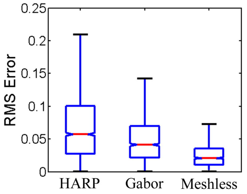
RMS error of computed circumferential strain in the numerical phantom.
In addition, we tested the 3D motion tracking performance of the proposed motion tracking method on in vivo cardiac data. Tagged MR images in multiple planes were obtained from a Siemens Trio 3T MR scanner with 2D grid tagging. The 3D tagged MR image set we used consisted of a stack of 5 SA image sequences, equally spaced from the base to the apex of LV, and 3 LA images, which were parallel to the LV long axis and with approximately 60 degree angles between one another. The motion tracking results are shown in Figure 12. Motion in two hearts, one normal and one of a LVH patient, was tracked for about 80% of the cardiac cycle (18 frames for the patient, 21 frames for the normal volunteer). First, notice that the magnitude of the contraction of the normal volunteer is larger than that of the LVH patient. Also notice that the normal heart’s contraction and dilation are essentially complete earlier than those of the LVH patient’s heart, as illustrated by the reconstructed 3D models at the same stages of the cardiac cycle. The black dots inside the LV mesh are control points driving the deformation of the underlying 3D meshless model. The geometric form of the LV model is based on the work in [23]. These 3D motion-tracking experiments show that the new motion tracking method is capable of detecting both the magnitude difference and the motion pattern difference between normal volunteers and LVH patients.
Fig. 12.

Representative 3D cardiac model and motion reconstruction of a normal volunteer and a LVH patient. The first row shows the heart model reconstructed using the data of a normal volunteer. In the second row is the heart model of a LVH patient. In the bottom is a plot showing the corresponding evolution of the average magnitude of circumferential strains during the cardiac cycle. The models in the above two rows are generated at cardiac cycle sampling times: A (3%), B (19%), C (34%), D (50%), and E (66%). It is clear that the normal heart contracts more (as shown by the greater shortening in circumferential direction); the normal heart also contracts and relaxes faster than the patient’s heart.
Finally, we evaluated the timing performance and efficiency of the new tracking method, for both 2D and 3D implementations. For 2D experiments, the overall motion tracking process, which includes the Gabor filtering, the RPM, and evolution of the deformable model, takes less than two minutes for an image sequence of size 100 by 100 pixels by 10 phases on a desktop PC with 2.66GHz Dual 2 Core CPU. For 3D experiments, the total processing time is about 25 minutes for each dataset (a dataset includes about 5 SA image sequences and 3 LA image sequences).
IV. Discussion and Conclusion
In this paper, we have presented a novel motion tracking technique, which integrates Gabor filters, the RPM, and deformable models. The three methods are tightly integrated in order to achieve the best tracking performance to support quantitative cardiac analysis. The method has a robust performance on tagged numerical phantoms and in vivo tagged cardiac MRI images, and, in particular, it performs well in myocardial regions with large deformation. It has several advantages: First, the use of phase maps generated by the Gabor filters allows efficient detection and location of tag intersections as the input for RPM. Second, the use of RPM simplifies the motion tracking process and is capable of generating a smooth and relatively accurate transformation function as the initial state for deformable models. This process reduces the chance of false tag assignment, as compared with the traditional gradient-based tag tracking method alone. Third, the implicit deformable model integrates image, phase, and smoothness information to reconstruct the motion with more robustness and less chance of singularities. Fourth, the use of the displacement magnitude as the smoothness constraint improves the overall quality of motion tracking. And fifth, the method is readily extendable for 3D applications. Experimental results show a better performance compared with another, widely used, motion tracking technique, HARP, and its timing performance is acceptable for clinical applications.
We have begun extending the motion tracking method into 3D. More experiments and further validation, especially for in vivo pathological data sets, will be needed to fully evaluate the performance of the method, and to build toward potential clinical applications. However, our preliminary results are very encouraging.
Fig. 1.
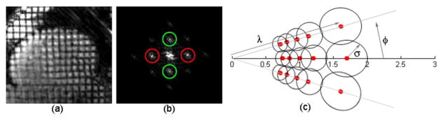
(a) A cardiac MRI image with grid tags. (b) The magnitude of the Fourier transform of the tagged MR image. Peaks inside red circles correspond to vertical tags and green circles to horizontal tags. (c) A bank of Gabor filters in the Fourier domain with parameters υ, θ and σ. The red dots represent centers of Gabor filters in the Gabor filter bank. The value on the horizontal axis is in the Fourier domain.
Acknowledgments
This work was partially supported by NIH grant R01 HL083309. We also thank Professor Gunaretnam Rajagopal for inspiring discussion on methodology details.
Contributor Information
Ting Chen, Email: chent4@umdnj.edu, Department of Radiology, New York University, New York, NY 10016 USA. He is now with the Cancer Institute of New Jersey, New Brunswick, NJ, 08901 (phone: 732-235-3513; fax: 732-235-8808;).
Xiaoxu Wang, Email: xiwang@cs.rutgers.edu, Department of Computer Science, Rutgers University, Piscataway, NJ 08854 USA.
Sohae Chung, Department of Radiology, New York University, New York, NY 10016 USA.
Dimitris Metaxas, Email: dnm@cs.rutgers.edu, Department of Computer Science, Rutgers University, Piscataway, NJ 08854 USA.
Leon Axel, Email: leon.axel@nyumc.org, Department of Radiology, New York University, New York, NY 10016 USA.
References
- 1.Axel L, Dougherty L. MR imaging of motion with spatial modulation of magnetization. Radiology. 1989;l7l:841–845. doi: 10.1148/radiology.171.3.2717762. [DOI] [PubMed] [Google Scholar]
- 2.Axel L, Dougherty L. Improved method of spatial modulation of magnetization (SPAMM) for MRI of heart wall motion. Radiology. 1989;l72:349–350. doi: 10.1148/radiology.172.2.2748813. [DOI] [PubMed] [Google Scholar]
- 3.Osman NF, McVeigh ER, Prince JL. Imaging heart motion using Harmonic Phase MRI. IEEE Trans on Medical Imaging. 2000 Mar;19(3):186–202. doi: 10.1109/42.845177. [DOI] [PubMed] [Google Scholar]
- 4.Gabor D. Theory of communication. J IEE. 1946;93(3):429–57. [Google Scholar]
- 5.Chen T, Axel L. Using Gabor filters bank and temporal-spatial constraints to compute 3D myocardium strain. Proceedings of EMBC. 2006 doi: 10.1109/IEMBS.2006.259875. [DOI] [PubMed] [Google Scholar]
- 6.Amini AA, Chen Y, Elayyadi M, Radeva P. Tag surface reconstruction and tracking of myocardial beads from SPAMM-MRI with parametric B-spline surfaces. IEEE Trans on Medical Imaging. 2001;20(2):94–103. doi: 10.1109/42.913176. [DOI] [PubMed] [Google Scholar]
- 7.Chui H, Rangarajan A. A new point matching algorithm for non-rigid registration. Computer Vision and Image Understanding. 2003;89(2–3):114–141. [Google Scholar]
- 8.Gold S, Rangarajan A. A graduated assignment algorithm for graph matching. IEEE Trans Pattern Analysis and Machine Intelligence. 1996;18(4):377–388. [Google Scholar]
- 9.Axel L, Chen T, Manglik T. Dense myocardium deformation estimation for 2D tagged MRI. In Proceedings of Functional Imaging and Modeling of the Heart. 2005:446–456. [Google Scholar]
- 10.Chen T, Chung S, Axel L. 2D motion analysis of long axis cardiac tagged MRI. Proceedings of Medical Image Computing and Computer-Assisted Intervention. 2007:469–476. doi: 10.1007/978-3-540-75759-7_57. [DOI] [PubMed] [Google Scholar]
- 11.Declerck J, Feldmar J, Ayache N. Definition of a 4D continuous planispheric transformatin for the tracking and the analysis of the LV motion. Medical Image Analysis. 1998:197–213. doi: 10.1016/s1361-8415(98)80011-x. [DOI] [PubMed] [Google Scholar]
- 12.Belytschko T, Krongauz Y, Organ D, Fleming M, Krysl Pl. Meshless methods: an overview and recent developments. Computer Methods in Applied Mechanics and Engineering. 1996:3–47. [Google Scholar]
- 13.Muller M, Keiser R, Nealen A, Pauly M, Gross M, Alexa M. Point based animation of elastic, plastic and melting objects. Proceedings of the 2004 ACM SIGGRAPH/Eurographics symposium on Computer animation. 2004:141–151. [Google Scholar]
- 14.Metaxas D. Physics-based deformable models: application to computer vision, graphics and medical imaging. Springer; 1996. [Google Scholar]
- 15.Wahba G. Spline models for observational data. Philadelphia: Society for Industrial and Applied Mathematics; 1990. [Google Scholar]
- 16.Wang X, Chen T, Metaxas D, Axel L. Meshless deformable models for LV motion analysis. Proceedings of the IEEE Computer Society Conference on Computer Vision and Pattern Recognition. 2008 doi: 10.1007/978-3-540-85988-8_76. [DOI] [PubMed] [Google Scholar]
- 17.Park J, Metaxas D, Axel L. Volumetric deformable models with parameter functions: a new approach to the 3D motion analysis of the LV from MRI-SPAMM. proceedings of ICCV. 1995:700–705. [Google Scholar]
- 18.Young A. Model tags: direct 3d tracking of heart wall motion from tagged magnetic resonance images. Medical Image Analysis. 1999;(3):362–371. doi: 10.1016/s1361-8415(99)80029-2. [DOI] [PubMed] [Google Scholar]
- 19.Mcinerney T, Terzopoulos D. A dynamic finite element surface model for segmentation and tracking in multidimensional medical images with application to cardiac 4D image analysis. Computerized Medical Imaging and Graphics. 1995;(19):69–83. doi: 10.1016/0895-6111(94)00040-9. [DOI] [PubMed] [Google Scholar]
- 20.Lancaster P, Salkauskas K. Surfaces generated by moving least squares methods. Mathematics of Computation. 1981:141–158. [Google Scholar]
- 21.Tustison NJ, Amini AA. Biventricular myocardial strains via nonrigid registration of anatomical NURBS models. IEEE Trans Med Imaging. 2006;25(1):94–112. doi: 10.1109/TMI.2005.861015. [DOI] [PubMed] [Google Scholar]
- 22.Schaefer S, McPhail T, Warren J. Image deformation using moving least squares. Proceedings of the 2006 ACM SIGGRAPH. 2006:533–540. [Google Scholar]
- 23.Haddad R, Clarysse P, Orkisz M, Croisille P, Revel D, Magnin IE. A realistic anthropomorphic dynamic heart phantom. Computers in Cardiology. 2005:801–804. [Google Scholar]
- 24.Chandrashekara R, Mohiaddin R, Rueckert D. Analysis of 3-D myocardial motion in tagged MR images using nonrigid image registration. IEEE Trans Med Imaging. 2004;23(10):1245–1250. doi: 10.1109/TMI.2004.834607. [DOI] [PubMed] [Google Scholar]
- 25.Frangi AF, Rueckert D, Schnabel JA, Niessen WJ. Automatic construction of multiple-object three-dimensional statistical shape models: application to cardiac modeling. IEEE Trans Med Imaging. 2002;21(9):1151–1166. doi: 10.1109/TMI.2002.804426. [DOI] [PubMed] [Google Scholar]
- 26.Yan P, Sinusas A, Duncan JS. Boundary element method-based regularization for recovering of LV deformation. Medical Image Analysis. 2007;11(6):540–554. doi: 10.1016/j.media.2007.04.007. [DOI] [PubMed] [Google Scholar]