Robust Encoding of Stimulus Identity and Concentration in the Accessory Olfactory System

Abstract

Sensory systems represent stimulus identity and intensity, but in the neural periphery these two variables are typically intertwined. Moreover, stable detection may be complicated by environmental uncertainty; stimulus properties can differ over time and circumstance in ways that are not necessarily biologically relevant. We explored these issues in the context of the mouse accessory olfactory system, which specializes in detection of chemical social cues and infers myriad aspects of the identity and physiological state of conspecifics from complex mixtures, such as urine. Using mixtures of sulfated steroids, key constituents of urine, we found that spiking responses of individual vomeronasal sensory neurons encode both individual compounds and mixtures in a manner consistent with a simple model of receptor–ligand interactions. Although typical neurons did not accurately encode concentration over a large dynamic range, from population activity it was possible to reliably estimate the log-concentration of pure compounds over several orders of magnitude. For binary mixtures, simple models failed to accurately segment the individual components, largely because of the prevalence of neurons responsive to both components. By accounting for such overlaps during model tuning, we show that, from neuronal firing, one can accurately estimate log-concentration of both components, even when tested across widely varying concentrations. With this foundation, the difference of logarithms, $\log A-\log B=\log \frac{A}{B}$, provides a natural mechanism to accurately estimate concentration ratios. Thus, we show that a biophysically plausible circuit model can reconstruct concentration ratios from observed neuronal firing, representing a powerful mechanism to separate stimulus identity from absolute concentration.

Introduction

Sensory systems have a remarkable ability to extract relevant information from a noisy and inconsistent environment. For example, the visual system is able to identify an object despite variability in observation angle or size (Riesenhuber and Poggio, 2002). A sound can be identified independent of volume or intensity (Barbour, 2011), and a smell can be recognized as a particular odor over a range of concentrations (Engen and Pfaffmann, 1959; Slotnick and Ptak, 1977; Bhagavan and Smith, 1997). Sensory stability, particularly in the face of changing conditions, has been subject to numerous investigations in multiple sensory systems, including olfaction (Stopfer et al., 2003; Wilson and Mainen, 2006; Uchida and Mainen, 2007; Cleland et al., 2011).

A central mystery is how olfactory percepts can be relatively constant despite dramatic changes in the raw peripheral representation of odors as stimulus concentration is varied (Wachowiak and Cohen, 2001). In principle, one possible computational strategy is through the use of ratios: if an odor has two components, A and B, the ratio of their concentrations is constant even if the absolute concentration is subject to environmental influences. This notion is supported by behavioral observations, such as the attraction of moths to particular pheromone blends (Baker et al., 1976) and the ability of rats to make choices based on ratios of components (Uchida and Mainen, 2007).

How might a neural system represent ratios? One possibility is through the use of logarithms; the log of a ratio is equal to the difference of logarithms as follows: $\log \frac{A}{B}=\log A-\log B$. This requires neural circuitry to represent the logarithm of concentration and compute a difference, which could be accomplished through inhibitory circuitry. Logarithmic representation of sensory stimuli has a long history, dating back to early psychophysicists Weber and Fechner (Fechner et al., 1966) and has been previously proposed as a neural mechanism for computing ratios (Brody and Hopfield, 2003; Uchida and Mainen, 2007). However, to our knowledge, no direct neural evidence of logarithmic or ratio coding exists in an olfactory system.

Here we explored the potential computation of logarithms and ratios by the accessory olfactory system (AOS), an independent olfactory system present in most terrestrial vertebrates. The AOS detects social cues from complex mixtures of stimuli. These cues are used by organisms to make behavioral decisions about reproduction and aggression conditional upon the status of other members of the social group. Behavioral and physiological state is known to be reflected in changes in the relative concentrations of components of stimuli, such as urine (Nodari et al., 2008), but absolute concentrations are expected to be highly variable (Hurst and Beynon, 2004) (see Fig. 1). Using multielectrode array recordings of accessory olfactory sensory neurons located in the vomeronasal organ (vomeronasal sensory neurons [VSNs]), we demonstrate that a logarithmic representation of concentration, and in turn log-ratio of concentration of two components, may be robustly calculated from the firing rates of VSNs. These results demonstrate the feasibility of quantitative “olfactory scene segmentation” using the responses of neurons with mixed selectivities for individual odorants.

Figure 1.

VSNs respond to a wide range of concentrations A, An example of environmental uncertainty facing the AOS. The concentration of ligands measured in a pool of urine of volume V depends strongly on environmental uncertainties, such as evaporation. However, ratios allow for robust representation of concentration invariant to environmental uncertainties. B, A population of idealized cells with slightly different sensitivities to the same compound are shown (top). Summing their activity produces a result that is linear with respect to log-concentration (bottom) over the range spanned by the cells. C, An example voltage trace from a single electrode in response to Ringer's solution control (top) and Q3910 (bottom). The tissue was stimulated for 10 s. D, Summary of average firing rates in response to presented stimuli in the same cell as shown in C. Error bars correspond to the SEM. E, A raster plot of the same cell shown in C and D in response to two negative controls and nine concentrations of two different sulfated steroids. Each stimulus was presented five times (rows within each block). Average firing rate is shown on the right.

Materials and Methods

Solutions and stimuli

We stimulated mouse VSNs using sulfated steroids (Nodari et al., 2008) purchased from Steraloids. All other chemicals were obtained from Sigma, unless otherwise indicated. Stock solutions of steroids were dissolved in either methanol or deionized water. The following steroids, referred to by their Steraloids catalog number, were used: A0225, Q1570, and Q3910. The exact molecular identities of these compounds are as documented previously (Nodari et al., 2008; Meeks et al., 2010). Ringer's solution contained 115 mm sodium chloride, 5 mm potassium chloride, 2 mm calcium chloride, 2 mm magnesium chloride, 25 mm sodium bicarbonate, 10 mm HEPES, and 10 mm d-(+)-glucose and was equlibrated by bubbling with 95% O₂/5% CO₂. High potassium Ringer's solution substituted 50 mm potassium for equimolar sodium.

Electrophysiological recording

Adult male mice 8–21 weeks of age of the B6D2F1 strain (The Jackson Laboratory) were used in all recordings. All experimental protocols followed the United States Animal Welfare Acts and National Institutes of Health guidelines and were approved by the Washington University Animal Studies Committee.

Dissection and recording procedures were performed as previously described (Holy et al., 2000; Nodari et al., 2008; Arnson et al., 2010); briefly, intact vomeronasal epithelia were isolated and mounted on a multielectrode array. The vomeronasal epithelium was removed from the bony capsule, the neuroepithelium was mechanically dissected as an intact sheet from the basal lamina. It was then held in place on the electrode array using a nylon mesh. Sulfated steroids were diluted with Ringer's immediately before the recording session. Sulfated steroids were used at nine concentrations, ranging from 10 nm to 100 μm, in approximately threefold increasing intervals. Binary mixtures were prepared by making mixtures of chosen dilutions of pure compounds, so that each individual mixture component was half the concentration of the original solution of pure compound. The following mixtures were used (all in μm): 5:5, 50:50, 15:5, 5:15, 0.05:0.5, 1.5:15, 0.5: 0.05, 15:1.5, 0.5:50, 0.05:5, 50:0.5, 5:0.05. Final methanol concentration in the stimulus solution was never >0.1%. All experiments included a minimum of two negative control (Ringer's) stimuli as well as a vehicle control containing 0.1% methanol in Ringer's solution. A positive control of Ringer's solution containing 50 mm potassium was also used. Stimuli were dispensed using an HPLC pump (Gilson 307) (Gilson), and a robotic liquid handler (Gilson 215) capable of taking samples from prepared tubes and injecting them in an HPLC valve (Gilson 819 injection module). This robot was controlled by the Gilson 735 software. Continuously bubbled Ringer's solution alternated with stimuli to produce continuous flow over the epithelium; the flow was heated to a temperature of 35°C and aimed directly at the epithelium. The timing of stimulus delivery (HPLC valve switch) was monitored electrically and fed back to the acquisition software. Stimuli were presented for 10 s in a block-randomized order. Delivery was repeated in a newly randomized order 4–6 times.

Extracellular recording was performed using multielectrode planar arrays (ALA Scientific Instruments) (10 μm flat titanium nitride electrodes isolated with silicon nitride) where electrodes were 30 μm apart, in two fields of 6 × 5 electrodes each. Electrical signals were amplified with a MEA 1060 amplifier (ALA Scientific Instruments), acquired at 10 kHz with a data acquisition card (National Instruments), and saved to disk. We used custom data acquisition and data analysis software based on COMEDI (http://www.comedi.org) and MATLAB (MathWorks).

Data analysis

Spike sorting.

This and all subsequent analyses were performed in MATLAB (Mathworks). After acquisition, single units were isolated using custom software. Spikes were sorted based on waveform shape across all electrodes using methods similar to those described previously (Marre et al., 2012). All single units had clear refractory periods of ∼25 ms or more.

Determining firing rate.

Change in firing rate of a cell, Δr, was calculated using a time window of variable length, set independently for each distinct stimulus. The window started with stimulus onset and ended at the point yielding the maximum firing rate, averaged over the window and across all trials of this stimulus. The time window was constrained to be at least 1 s in duration and at most 15 s after stimulus onset. A baseline firing rate was computed by averaging the firing rate across trials for 10 s before stimulus delivery. The Δr value was calculated by subtracting the baseline firing from the peristimulus firing rate. Because of time lags within the delivery system and variability in the placement of the stimulus pipette, an offset was allowed between the time at which stimulus delivery began and stimulus reached the tissue. The offset was determined by measuring the activity across all electrodes in a particular recording using 250 ms time bins. The offset was set as the time bin before an increase in net activity after stimulus delivery onset, with values ranging from 1.25 to 4.75 s.

A response was determined to be statistically significant if it differed from the Ringer's control using a rank-sum test with a p value threshold of 0.05 with a minimum Δr of 2 Hz. To control for methanol and Ringer's artifacts, Δr was computed for the vehicle and Ringer's solution stimuli. No cells in this dataset were found to have a significant Ringer's or vehicle response. Because of the large number of stimuli and cells examined (see below), to further exclude false positives we used the Hill equation (described in more detail below) to model the response of each cell to the stimulated compounds based on the fits described below. Cells with predicted firing rates not exceeding 1 Hz at any concentration were excluded from further analysis. A total of 22 cells were excluded in this round (4.4% of the total population, consistent with a statistical cutoff of p = 0.05). By eye, none of the excluded cells appeared to be responsive.

Concentration characterization.

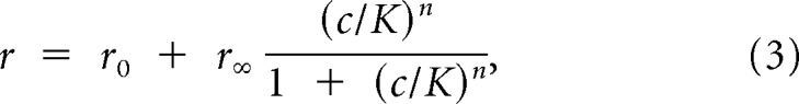
To compute the response properties of individual cells, the change in firing rate in response to a range of concentrations was fit with three models: a log-concentration model, a rectified log-concentration model, and a Hill model. The validity of the model was verified using the p value computed from the χ² statistic. As the null hypothesis is that the model is an accurate descriptor of the data, a p value greater than our significance criteria (i.e., 0.05) indicates that the model provides a reasonable fit. The log-concentration model, a model in which the firing rate rises linearly with the logarithm of concentration, was computed by fitting the cell's firing rates (r) across concentrations to the equation, $r=\alpha \log \frac{c}{c_{ref}}+\beta$, where α is the slope (Hz), c is the stimulus concentration (m), c_ref is a normalizing factor to make concentration unit-less and is equal to 1 m, and β is the y-intercept when c = c_ref (Hz). Firing rates computed on each trial were used (4–6 per stimulus).

The rectified log model differed from the above model in that below a minimum concentration threshold, c₀, firing was equal to a baseline firing rate r₀, or if c < c₀, r = r₀ and if $c\ge c_0,r=\alpha \log \frac{c}{c_0}+r_0$.

The Hill equation fit was calculated by fitting the firing rate of the cell to the Hill equation,

where r₀ is the baseline firing rate, r_∞ is the maximum firing rate for the cell, c is the stimulus concentration, K is the binding affinity of the cell to each ligand, and n is the Hill coefficient. Using the 4–6 repeats of each concentration of each single steroid stimulation, r₀, r_∞, K, and n were all fit to minimize χ². We started from a simplified “flat” model, progressing to a linear model, a Hill model with n = 1, and finally the full Hill model. This progressive increase in the number of parameters reliably led to fits that, by eye, appeared consistent with the global optimum and avoided getting trapped in local minima. The value of n, indicating cooperativity, was initially allowed to be between 0 and 5. We found that cells with n values at or near 5 consistently were responsive only to the highest concentration, providing too little data to constrain model parameters. These cells were excluded from all analyses involving the Hill parameters. For subsequent analyses, these cells were refit with the Hill model with a fixed n of 1. Importantly, when fitting the responses of a cell to two different pure compounds, the only parameter that was permitted to differ for the two compounds was K; the remaining parameters were jointly optimized for both compounds. This choice effectively posits that the ligands are acting at the same binding site and that the Hill coefficient, maximum, and minimum firing rates are generic properties of the receptor neuron. In other olfactory systems, violations of these assumptions have been observed (i.e., Ache and Young, 2005; Rospars et al., 2008), but our VSN data are well described by this model (see Figs. 2 and 4). In the absence of evidence to the contrary, we therefore confined our analyses to this simple model.

Figure 2.

Single neuron encoding of log-concentration. A, Top, Simulated cell with a “typical” Hill-response profile (black line). To demonstrate that the concentrations around the EC₅₀ approximate log-concentration, we fit the response with a rectified-log model (red dotted line). Bottom, Another simulated cell with a smaller Hill coefficient. This cell approximates log-concentration over the entire range shown (red dotted line). B, Goodness of fit to the Hill model for each VSN as measured by the 1/p value to the χ² fit. Cells below the dotted line (p = 0.05) are well described by the model (n = 47 neurons from 18 mice). C, Hill coefficients for each VSN. D, EC₅₀ to each compound. E–G, Example cells with a rectified-log model (red dotted line) or an unrectified log model (blue dotted line). H–J, Reconstruction of log-concentration using the response of the cell to the left. Whereas J provides a reasonable approximation of log-concentration, I does so only at a few higher concentrations and H does only at nonresponsive concentrations.

Figure 4.

Competitive binding. A, The response of a cell to a range of concentrations of Q1570 (top) and Q3910 (bottom). B, The response of the same cell to binary mixtures of Q1570 and Q3910 (black). Using the Hill model parameters fit to this cell previously, we predicted the expected firing rate to these mixtures given that the cell follows competitive binding (gray). The model fit and recorded rates closely agree, providing evidence for the competitive binding model. C, The recorded response (left side of each column) and predicted response (right side of each column) to sulfated steroid mixtures across the population of 24 cells from 18 mice.

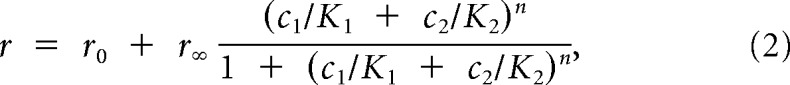
Mixtures were also fit with a Hill model incorporating competitive binding of different compounds within the mixture,

using r₀, r_∞, K, and n values from the pure compound Hill equation fits. Because the validity of the Hill equation fit requires approximate saturation to at least one tested compound, only the 24 most sensitive cells were used to investigate competitive binding. Saturation was determined by a K value of ≤10 μm.

Log-concentration modeling.

To determine whether populations of VSNs could be used to reconstruct log-concentration, we used a linear model, log(ĉ) = w · r where ĉ is an estimate of the concentration presented, r is a vector containing the responses of each cell to the presented concentration of that compound, and w is the vector of weights, n_cells long. When analyzing mixtures of two ligands, we seek two w vectors, w₁ and w₂, so that the estimated log-concentration of ligand 1 is w₁ · r and w₂ · r for ligand 2. Only cells that had an EC₅₀ value < 100 μm for at least one compound, indicating a cell that was responsive over the presented range of concentrations, were used (n = 56 cells). Weights ranged from −0.52 to 1.3 Hz.

Model parameters (the weights w_i) were set using two procedures. First, we explored a “self-tuning” approach, using the pure compound responses for compound i to tune the weight vector w_i. We generated a matrix of firing rates, R, one for each trial (4–6 trials) per concentration per cell. We used a concentration vector, c, covering the range from 300 nm to 100 μm in increments of half log units. w was tuned using linear least-squares regression for each compound individually, yielding two w vectors in which each cell has two weights, one for each compound. The model efficacy was first tested using the aforementioned weights and average firing rates for all cells in response to each sulfated steroid when presented independently. The model was also tested using the firing rate for each cell in response to the mixture of components. To find the reproducibility of reconstruction, we recalculated concentration using leave-one-out cross-validation by using an average firing rate obtained by sampling 4 of 5 repeats. This allows for model verification taking into account the full extent of sample variability and guards against overfitting. Samples were drawn randomly 100 times, and the response was averaged. The error bars correspond to the SE. All error values shown are calculated as E = Σ(log c_actual − log ĉ_model)², summed across all stimuli and concentrations.

“Self-tuning,” although straightforward, cannot properly handle mixtures; this can be demonstrated using a simple toy model of neuronal responses. Suppose that the population firing rate to pure compound 1 is r₁ = a₁log(c₁), where a₁ is an arbitrary vector and c₁ is the actual concentration of compound 1; compound 2 behaves likewise with a different arbitrary vector a₂. Suppose further that a mixture of these two compounds results simply in the sum of these firing rates, r = r₁ + r₂. Using the mixture data, we would estimate the log-concentration of each compound as follows:

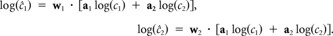Perfect “self-tuning” for this toy model implies w_i · a_i = 1. However, to yield the correct result for mixtures, we require the additional constraints w₁ · a₂ = 0 and w₂ · a₁ = 0; these constraints are not imposed by the least-squares fit when each weight vector is tuned independently. These constraints can be (approximately) satisfied if the neurons have no overlapping stimulus responses, but it does not happen naturally when at least some neurons respond to both ligands.

Consequently, we developed an alternate procedure, which we call “cross-tuning,” designed to account for neurons that have overlapping responses. This procedure also accounts for neurons that violate the simplistic assumptions of the above toy model. In its most general form, the strategy is to use single-compound responses to fit a model describing the neuron's response properties, and then use the parameters to “simulate” responses to all possible tested mixtures. The simulated mixture responses are used in a least-squares sense to train the weight vectors to properly extract the log-concentration of each component. The model is then tested by comparing its reconstruction of log-concentration using actual mixture data.

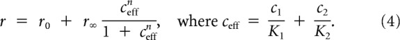
More specifically, we calculated predicted mixture responses based on the Hill mixture model presented above, using the efficacy c_eff = c₁/K_1i + c₂/K_2i for the ith neuron. For a particular simulated mixture and neuron, we computed c_eff. To include the effects of noise, we estimated firing rate responses using a “lookup table” procedure: we compared this efficacy with all of the efficacies tested with pure compound A and pure compound B, and the closest match was chosen to assign the Δr values for all simulated trials of this particular simulated mixture for this neuron. This was repeated for all possible mixtures (using concentrations ranging from 300 nm to 100 μm in half-log units) and all cells. This yielded a “response vector” of length 180 (36 mixtures and 5 trials) for each cell, or in total a 180 × n cells R matrix. Finally, least-squares minimization to reconstruct the actual concentrations of each component of the simulated mixtures was used to solve for w₁ and w₂.

Ratio computation.

Ratios were computed using the reconstructed log-concentrations. For each mixture, the reconstructed log-concentrations for each compound were subtracted to give the log-ratio as follows: $\log {\widehat{c}}_1-\log {\widehat{c}}_2=\log \frac{{\widehat{c}}_1}{{\widehat{c}}_2}$. Error bars were computed as described above.

Results

The accessory olfactory system, like all other sensory systems, must be capable of representing information in a way that is robust to environmental uncertainties. Here, we explore the possibility that the activity of sensory neurons can be used to compute concentration ratios, as the ratio is insensitive to absolute changes in concentration yet still sensitive to relative changes (Fig. 1A). As an initial step, we explore the degree to which the logarithm of concentration, a natural stepping-stone to computing ratios, might be represented. In principle, this may be achieved by individual VSNs, or alternatively as a consequence of population activity (Fig. 1B).

We began by investigating how individual sensory neurons represent concentration across the large dynamic range of the system. We performed multielectrode array recordings of VSNs in response to three sulfated steroids: two glucocorticoids (Q1570 and Q3910, two “similar” odors) and one androgen (A0225, a more “dissimilar” odor). Each preparation was tested with two of these stimuli, each over a wide range of concentrations, and with binary mixtures of the two compounds. As has been previously reported (Nodari et al., 2008; Arnson et al., 2010; Meeks et al., 2010; Celsi et al., 2012; Turaga and Holy, 2012), we observed that sulfated steroids induced activity in VSNs. Of 494 total cells (n = 18 mice), 95 were responsive to at least one sulfated steroid (rank-sum test, p < 0.05, see Materials and Methods).

Individual neurons provide poor representation of log-concentration across a large dynamic range

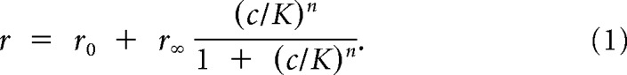
Receptor–ligand interactions are frequently described by a Hill model (Firestein et al., 1993; Wilson and Mainen, 2006). Qualitatively, this model captures three regimens: one at low concentrations in which little or no response is observed, a rising phase where response increases with increasing ligand concentration, and a high-concentration regimen in which the response saturates. Applied to the spiking rate of neurons, the Hill model can be written as follows:

where r is the firing rate, c indicates ligand concentration, K corresponds to the concentration at which the half-maximal response is achieved (EC₅₀), r₀ is the spontaneous firing rate, r_∞ is the maximum stimulus-induced increase in firing rate, and n reflects the receptor cooperativity. Using this model, the response can be viewed as being approximately linear with respect to log-concentration near EC₅₀. The extent of approximately linear behavior depends on the Hill coefficient, n; larger values of n correspond to a more narrow dynamic range (Fig. 2A, top), whereas smaller values indicate a larger concentration span over which the response is approximately log-linear (Fig. 2A, bottom). To investigate whether individual sensory neurons can represent log-concentration across the large dynamic range, we explored the stimulus responses of a population of VSNs in terms of a Hill model.

We tested each VSN using two different sulfated steroids, at concentrations spanning four orders of magnitude, ranging from 10 nm to 100 μm (Fig. 1C–E). Of the 95 steroid-responsive cells, a sizable subset showed responses only to the highest concentrations, and thus the fitting parameters were not well determined by the data. Therefore, here we focused on the 47 cells for which EC₅₀ < 100 μm (for at least one of the two compounds) and n < 5. This group of cells was virtually synonymous with the subset responding to at least two of the presented concentrations. Each neuron's responses to both compounds was fit simultaneously to the Hill model (Eq. 3). The only parameter associated with the Hill model that differed with each compound was K, or EC₅₀, where K₁ and K₂ describe the EC₅₀ to each of the two compounds. Quality of fit was measured by the p value of the χ² fit, as shown in Figure 2B. For 42 of 47 cells (89%), the Hill model served as a plausible description of their response, in the sense that this model could not be statistically discounted (p > 0.05). The Hill coefficient, n, ranged from 0.39 to 4.9, with the majority (23 of 42) falling between 0.5 and 2 (Fig. 2C). The EC₅₀ varied from 7.7 × 10⁻⁸ to 1 × 10⁻¹ m across the population; EC₅₀s >1 × 10⁻⁴ m, the highest stimulated concentration, indicated that the cell was not responsive to that particular compound (Fig. 2D).

As the value of n directly influences the dynamic range of the neuron, we considered individual neurons with high, medium, and low n values (Fig. 2E–G, respectively). We fit each cell with a rectified log model (see Materials and Methods) to test whether any portion of the cell's response was approximately log-linear (red dotted line). As shown in Figure 2E, the cell with a high n (n = 4.9) did not exhibit any sizable span over which the response was approximately log-linear, and an attempt at reconstructing log-concentration using a linear relationship (see Materials and Methods) exhibited very large errors (Fig. 2H; mean 0.9 log units of error, maximum 1.81). A mid-range cell (n = 2.0) showed approximately log-linear behavior over a larger concentration range (Fig. 2F). The activity of this neuron could be used to reconstruct log-concentration with slightly better accuracy (Figure 2I; mean 0.7 log units of error, maximum 1.1). A low n cell (n = 0.76) appeared to be reasonably log-linear across the tested range (Fig. 2G). We were able to decode log-concentration from this cell with an average error of 0.4 log-units, with a maximum difference of 0.8 log-units (sixfold). For this particular cell, a log-linear model, $r=m\log \frac{c}{c_0}$, was a statistically plausible (p > 0.05) fit. Of 95 responsive cells, from an initial population of 494 cells, we observed only three cells that appeared to respond log-linearly over such a wide concentration range (3% of responsive cells, 0.6% of all cells). None of the neurons that were stimulated by the androgen compound, A0225, displayed this property. Although it is possible that a rare, specialized population encoding log-concentration exists, it is unclear whether the accessory olfactory system could rely on such neurons for general ratio computation. Consequently, we also explored the possibility of population coding for log-concentration.

Populations of VSNs can reliably represent log-concentration across a large dynamic range

We tested the idea that populations of neurons could be used to reconstruct log-concentration by using a linear model in which the estimated log-concentration, log ĉ, is calculated as log ĉ = w · r, where r is the vector of firing rates across the population and w is a vector of weights. We measured the firing rate of each cell in the population (Fig. 3A) to the different concentrations (see Materials and Methods) of a sulfated steroid (i.e., A0225); we then optimized the match between the estimated log ĉ and the actual log c by least-squares, thereby solving for the weights. Using the response of each cell to compounds presented individually, we were able to reconstruct log-concentration as shown in Fig. 3B, C. The reconstructed concentration differed from the actual concentration by at most 0.28 log units, less than twofold, over three orders of magnitude. Compared with the concentration representation by individual cells (Fig. 2H–J), this scheme proved to be substantially more accurate and robust over a larger range of concentrations, from 300 nm to 100 μm. This suggests that populations of sensory neurons may be better suited to the task of accurately representing concentrations than are individual neurons.

Figure 3.

Population coding of log-concentration. A, The activity of 25 cells from 18 mice that were stimulated with 10 μm A0225, sorted by response magnitude. B, The actual concentration presented (black) and the model reconstruction (gray). C, Using the firing rates obtained in response to six different concentrations of a sulfated steroid presented individually, log-concentration was accurately reconstructed.

Neuronal responses to stimulus mixtures

Natural stimuli for the AOS, such as urine and other secretions, are complex mixtures (Kimoto et al., 2005; Chamero et al., 2007; Nodari et al., 2008). Estimating the relative concentrations of individual components in such mixtures is expected to be far more complex and is a problem that, in terms of actual neuronal recordings, appears to have received little or no attention.

To explore how mixtures are represented, we presented VSNs with mixtures of two similar (Q1570 and Q3910) or two dissimilar (Q1570 and A0225) sulfated steroids at differing concentrations and proportions (for details, see Materials and Methods). The two similar compounds have previously been shown to activate overlapping populations of neurons (Meeks et al., 2010; Turaga and Holy, 2012), representing a challenging decoding problem with ambiguity in the meaning of each neuron's response. The two dissimilar compounds activate largely nonoverlapping populations (data not shown), which might be expected to be a simpler decoding problem.

In addition to the mixtures, each neuron was presented with each pure compound, allowing us to fit the parameters of a Hill model (Fig. 4A). We modeled the response to mixtures in terms of a competitive binding model,

The response to the mixture can be predicted based on the parameters of the fit to pure-compound responses. To test this model, only responsive cells that showed saturation to one or more compounds were used (n = 24 cells) (see Materials and Methods). An example cell's predicted response compared with the actual response is shown in Figure 4B, suggesting that this particular cell was well fit by the competitive binding model. The actual responses and predicted fits are shown for the population of cells in Figure 4C. A majority of recorded cells (16 of 24) were tolerably well described by this model (p > 0.001, χ² test), and poorly fitting cells did not have any obvious systematic departure from the competitive binding model (Fig. 4C). It is also worth noting that when we refit the Hill parameters to the aggregate pure-compound and mixture data (using Eq. 2), the majority (19 of 24 cells) were well described (p > 0.05; χ² -test). This suggests that this model provides a reasonable description of the responses. In what follows, we use the more strenuous test of generalizability, where the parameters are fit using only pure-compound data, and then applied to the analysis of mixture data.

Populations of VSNs encode log-concentration of mixture elements

These results show that population activity of sensory neurons can be used to estimate log-concentration of sulfated steroids across a range of concentrations. Because natural stimuli exist as mixtures of active ligands, ultimately we are interested in knowing whether concentration of the individual components can be reconstructed from responses to a mixture. Therefore, we tested whether the same model as previously described, log ĉ_i = w_i · r, suffices to reconstruct the log-concentration of all mixture elements (where the subscript refers to the ith compound) from a single set of neuronal responses r.

Crucially, we tuned the weights without “access” to the measured firing rates to mixtures, as we wished to use these responses as an independent test. We therefore limited our tuning dataset to responses recorded to each pure compound, across all concentrations. We first considered a “self-tuning” model, in which w₁ was tuned using responses to compound 1 but blind to the responses to compound 2, and likewise for w₂. This model reproduces the pure compound log-concentrations well (Fig. 3C) but performs relatively poorly on the mixtures, particularly in decoding the Q1570 compound (Fig. 5). The model reconstruction differed from the actual concentration used by as much as 2.57 orders of magnitude, and consistently underestimated Q1570 by at least half a log unit. A likely cause of this poor performance is the fact that some cells respond to both ligands, but tuning the weights for each compound independently does not take this into account (see Materials and Methods).

Figure 5.

Log-concentration reconstruction from population response to mixtures. A, The response of a population of cells stimulated with 30 μm Q1570 (black) (25 cells, 18 mice) and 3 μm A0225 (gray), presented individually (top). Bottom, The response of the same population of cells to the mixture of the two compounds at half their concentrations (15 μm Q1570 and 1.5 μm A0225). B, Using weights set from responses to pure compounds, we tested the model with the responses to mixtures. The actual versus model reconstructed concentrations are shown. The model poorly reconstructs the concentration of both compounds. C, Mixture element concentration reconstruction using the same technique described in B across a larger range of concentrations. The reconstructed concentration does not appear to accurately capture the stimulated concentration across the range of stimuli.

We therefore implemented a “cross-tuning” model, in which the weights were tuned accounting for the possibility of mixtures. To implement this tuning without using the measured responses to mixtures, we used the Hill parameters to calculate the efficacy, c_eff (Eq. 4), for all possible mixtures (see Materials and Methods). Using the firing rates corresponding to the pure compound response closest to each efficacy, we obtained a “predicted” response profile for each mixture condition. Therefore, this is a “cross-tuning” model in the sense that an allowance is made in the least-squares procedure for the simultaneous presence of both compounds. However, all the data used to tune the parameters come from just the pure compound responses.

We then tested this cross-tuning model against firing rates obtained in response to mixtures. As before, this was done for both the “easier” case (Q1570 and A0225) and the “harder” case (Q1570 and Q3910). Because we did not make further adjustments in the parameters to improve the quality of the fit, this represents an independent test of the model. As shown in Figure 6, the cross-tuning model was considerably more effective than naive self-tuning. Over three orders of magnitude of concentration, the error ranged from 0.003 to 1.74 log-units (Q1570). This suggests that populations of VSNs could be used to represent both log-concentration and identity over a large range of concentrations.

Figure 6.

Population coding taking nonlinearities into account. A, Reconstructed versus actual concentration in response to the pure compounds of Q1570, A0225, and Q3910 presented individually. Error bars indicate SE (n = 63 cells from 18 mice). B, C, Reconstructed versus actual concentration of mixture components using two populations of neurons: 25 cells (B) and 38 cells (C). Using the recorded responses to mixtures, the model was able to disambiguate mixture elements and concentrations. D, The response of a population of cells to two sulfated steroids presented separately (30 μm Q1570 and 10 μm A0225). E, The response of the same population in the same order, to the mixture of the two compounds at half their original concentrations (15 μm Q1570 and 5 μm A0225). F, The model reconstruction of each element of the mixture compared with the actual concentrations of the mixture elements.

Model parameters

We explored the model parameters to identify what features the model emphasized when setting the optimal weights. In both populations of cells, a few cells were heavily used (Fig. 7A,B). This suggests that perhaps equivalent results might be obtained using only a subset of the neuronal population (Fig. 7C,D). To explore this dependence, we first identified the cell that was most accurate in reconstructing log-concentration. We then found the cell that, when combined with the first, reduced the error the most, and kept adding the “best” cells until all were used. In the first population of cells stimulated with Q1570 and A0225 (“easier” case), 81% of error reduction was accomplished with only three cells, indicating that a quite small subset suffices for reasonably accurate reconstruction. In the second population stimulated with Q1570 and Q3910 (“harder” case), the three “best” cells reduced the error by 62%. In both cases, the minimum error was obtained with a subset of neurons, 13 of 25 cells in the first case and 15 of 38 cells in the second, reflecting generalization error as the number of parameters in the model increased. In some cases, these “extra” cells incorporated beyond the minimum point were unreliable across trials; in other cases, they were redundant cells in that there was a more reliable cell with a very similar response profile that was more valuable in recreating log-concentration. This emphasis on more reliable cells can be observed in Figure 7E, F, which reveals that model weight varied inversely with estimated variance in the EC₅₀. The general trend across both populations was that cells with lower variance, or more reproducibility, tended to be used in the reconstruction more heavily.

Figure 7.

Contributions of individual neurons to reconstruction. A, B, Weight times the maximum firing rate of that cell, corresponding to throughput, or how much information the cell contributed. Each cell has two weights, one per compound. Cells are ordered based on maximum w × Δr; n = 25 cells from 9 mice (top) and n = 38 cells from 9 mice (bottom). C, D, Model error as a function of numbers of cells used (Q1570, A0225 top, Q1570, Q3910 bottom), starting with the most informative cells. Model error corresponds to the sum of squares error. E, F, Weight times maximum firing rate (as in A,B) as a function of variance in the fit of the EC₅₀ value in the Hill model fitting. The more reliable cells (with smaller variance) tend to be the most heavily used by the model.

Populations of VSNs can be used to represent ratios

Using the log-concentration responses, we tested whether log-ratios could be computed from VSN activity, based on the idea that log c₁ − log c₂ = log c₁/c₂. We used the log-concentrations decoded in response to sulfated steroid mixtures and compared the reconstruction with the actual log-ratio presented. As shown in Figure 8, the reconstructed ratios reflected the actual ratios. Ratios ranged from 1:1 to 1:100 with stimuli ranging from 300 nm to 100 μm. The greatest error observed was in the 1 μm:100 μm Q1570:Q3910 mixture, which differed from the actual value by 1.75 orders of magnitude. The correlation coefficient (r) of this dataset was 0.91, indicating a high degree of correlation. The Q1570:Q3910 population is a harder case in that cells responded to both compounds, often with equal affinity. Therefore, it is unsurprising that the reconstruction was slightly less accurate given the finite population of recorded cells (r = 0.843).

Figure 8.

Log-ratio reconstruction. A, Actual and model reconstructed ratio for an example ratio. The example mixture was of 5 μm Q1570 and 5 μm A0225. B, C, Actual versus model reconstruction of the log-ratio using two different populations of VSNs. Error bars indicate SEM and are typically smaller than the points; n = 25 cells from 9 mice (A, B) and n = 38 cells from 9 mice (C). r indicates the correlation coefficient. There is a high degree of correlation.

These results provide the first evidence, to our knowledge, that ratio and logarithmic coding in olfaction can be generated from actual neuronal responses, thus providing a robust encoding scheme for the accessory olfactory system.

Discussion

We have demonstrated that, in principle, the accessory olfactory system is capable of representing concentration information in a robust manner through the use of log-ratios. Activity of populations of VSNs can be weighted and summed to represent log-concentration and the log-ratio. In particular, with an appropriate model, it sufficed to tune the parameters using responses just to individual components; the resulting model was able to accurately reconstruct log-concentration of both components of mixtures. Using neuronal data recorded from sensory neurons, we demonstrated the viability of this coding scheme that allows the AOS to represent concentration in a robust manner that is both sensitive to changes in relative concentrations of stimuli yet insensitive to changes in absolute concentration.

The ability to reconstruct both identity and concentration of mixtures serves as a form of olfactory “scene segmentation” as we are able to discriminate and classify discrete elements of complex stimuli. Although this term is often used in the realm of visual neuroscience to refer to the ability to pick out objects from a complex environment, it is also applicable to olfaction as olfactory stimulus space is made up of diverse mixtures that are parsed by olfactory systems (Brody and Hopfield, 2003; Mainen, 2007). Although our model is used to identify and quantify only two compounds presented simultaneously, the framework can be applied to a higher-dimensional stimulus space.

Ratio coding and the accessory olfactory system

Ratio-computation is particularly well suited for the mouse AOS. This system is specialized to detect nonvolatile ligands present as mixtures in bodily substances, such as facial secretions and urine (Kimoto et al., 2005; Chamero et al., 2012). The VNO in the nasal cavity contains a blood vessel acting as a pump that draws liquid stimuli into contact with receptor neurons when the mouse makes direct contact with the stimulus (Meredith, 1994). In contrast, the main olfactory system detects volatile compounds. Differences in volatility between ligands will result in different rates of evaporation and therefore nonstable concentration ratios. The nonvolatile nature of AOS stimuli implies that these ligands do not evaporate when left in the environment. Although the absolute concentration of each ligand will vary with solvent (water) evaporation, the relative concentration of compounds will not change. Consequently, this presents an ideal system to use, and explore, ratio coding.

Biological plausibility of log-ratio coding

A strength of this model is that it is based on biologically plausible constructs. It incorporates weighted summation and subtraction, operations that can be readily accomplished via synaptic scaling, pooling, and a combination of excitatory and inhibitory circuitry. One prerequisite for log-encoding over a large concentration range is diversity in the sensitivities of different sensory neurons (Fig. 1B), a requirement that was met by our observed data (Fig. 2C). It is unknown whether these differences in sensitivities are the result of neurons expressing the same receptor with different expression levels (Cleland and Linster, 1999) or the result of expression of different, possibly closely related receptors, each with a different threshold. It is unlikely that this phenomenon results from combinatorial expression of multiple receptors as VSNs are thought to express one, or a few (Martini et al., 2001), types of receptors of ∼300 known varieties (Touhara and Vosshall, 2009).

From the VNO, it is known that receptor neurons project into glomeruli in the AOB in which an individual glomerulus receives input from only one type of receptor neuron (Belluscio et al., 1999; Rodriguez et al., 1999). Unlike in the main olfactory bulb, mitral cells, the projection neuron out of the AOB, receive input from multiple glomeruli. Based on anatomical data, whether these mitral cells receive redundant input (Del Punta et al., 2002), input from different receptor types (Wagner et al., 2006), input from similarly responsive sensory neurons, or some combination thereof is unknown. However, a comparison of sulfated steroid responses in VSNs versus in mitral cells in the AOB suggests that most processing streams largely maintain segregation, with a few cases of mixing observed (Meeks et al., 2010). This may support the notion that mixed inputs, when they exist, can serve to expand the dynamic range of the mitral cells but maintain the stimulus specificity of VSNs. Pooling of VSNs provides a potential locus for log-concentration representation in the AOS; thus, mitral cells may receive net excitatory input representing log-concentration.

The AOB also contains laterally-inhibitory circuitry (Hendrickson et al., 2008; Larriva-Sahd, 2008), which might in principle compute the difference between log-concentrations. Theoretically, a log-concentration representation of one compound at the glomerular or mitral cell level may provide inhibitory input onto another mitral cell. If this target cell is also receiving excitatory input representing log-concentration of a different compound, this cell could be the site of comparison (subtraction) of the two log-concentrations. Consequently, in the AOS, it seems possible that ratio-representation might be observed as early as the mitral cell level.

Concentration response of VSNs and logarithmic coding

Using multielectrode array recordings of sensory neurons in the VNO, we measured the response of a group of cells to a range of concentrations of sulfated steroids and binary mixtures. The response of individual neurons could be modeled using the Hill model, which has previously been used to describe sensory neuron activity in both the accessory (Holy et al., 2000; He et al., 2010; Celsi et al., 2012) and main olfactory systems (Firestein et al., 1993; Wilson and Mainen, 2006). The rising phase of a Hill-fit response approximates logarithmic coding, and potentially is a way in which the system could represent log-concentration. Indeed, a model of concentration invariance proposed by Hopfield (Hopfield, 1999; Brody and Hopfield, 2003) and directly applied to ratio coding by Uchida and Mainen (2007) is based on the idea that logarithmic coding can be approximated by receptor–ligand interactions from threshold to saturation. The activities of VSNs were fit with a rectified-log model (Fig. 2E–G). However, the concentration range over which the cells were linear varied across the population from a very narrow to a wider range (Fig. 2C,D), and many cells did saturate over our target concentration range. We did observe a few neurons that responded in a nearly log-linear fashion over our tested concentration range (Fig. 2G); however, these cells were very rare (n = 3 of 494 cells), and this pattern of activity was only observed in response to a subset of stimuli.

Population coding to represent log-concentration

Single-neuron encoding schemes face a major interpretive challenge: when a cell responds to more than one stimulus (Meeks et al., 2010; Turaga and Holy, 2012) (Fig. 1D), the readout of a neuron's response is ambiguous. For this reason, the diversity of activity of VSNs is ideal for a population-coding scheme that allows for a reliable representation of log-concentration across a large dynamic range. Our model implements a weighted summation of populations of sensory neurons to reconstruct log-concentration; log-ratios can then be computed by subtraction.

We identified a key computational challenge facing this system. Simply tuning the model weights in response to each compound individually yields poor results for mixtures (Fig. 5) because of the existence of neurons responding to both components of the mixture. Significantly better results are obtained when these overlaps are taken into consideration (Fig. 6).

This study extensively tested mixtures of two compounds. However, natural stimuli for the AOS, like urine, are complex mixtures of many compounds. Therefore, for this to be a realistic coding scheme, it must be capable of scaling to larger numbers of ligands. At the level of two compounds, the “cross-tuning” model's success emphasized the importance of accounting for the complete receptive field of individual neurons. For an arbitrarily large number of stimuli, what kind of interactions may occur at the receptor level and how might the system, or model, handle the diversity? VSN tuning is determined by receptor expression, and the receptors are activated by only a specific set of stimuli. Previous studies have demonstrated that VSNs respond to one or a few sulfated steroids when presented individually (Meeks et al., 2010; Turaga and Holy, 2012), implying that the response of single neurons will be determined by only a small number of compounds out of a complex mixture. This limits the scope of the “cross-tuning” required for more naturalistic, complex stimuli.

The log-concentration model essentially comes down to weighted summation, synaptic weights, and inhibitory circuitry, subtraction. How might the system set these weights? One possibility is that the AOS is wired in development to compute ratios: sensory neurons are pooled in glomeruli and lateral circuitry is established with specific strengths, set over the course of evolution. Another possibility is that experience shapes the computation, in which the AOS changes synaptic weights based on stimuli present in the environment or social cues that are relevant at particular times or environments.

This study is the first to demonstrate that both logarithmic and ratio coding can be obtained quantitatively from experimentally observed neuronal data. This represents a biologically plausible model in which populations of neurons can be used to achieve robust detection of concentration across a very wide dynamic range.

References

- Ache BW, Young JM. Olfaction: diverse species, conserved principles. Neuron. 2005;48:417–430. doi: 10.1016/j.neuron.2005.10.022. [DOI] [PubMed] [Google Scholar]
- Arnson HA, Fu X, Holy TE. Multielectrode array recordings of the vomeronasal epithelium. J Vis Exp. 2010;37 doi: 10.3791/1845. [DOI] [PMC free article] [PubMed] [Google Scholar]
- Baker TC, Cardé RT, Roelofs WL. Behavioral responses of male Argyrotaenia velutinana (Lepidoptera: Tortricidae) to components of its sex pheromone. J Chem Ecol. 1976;2:333–352. doi: 10.1007/BF00988281. [DOI] [Google Scholar]
- Barbour DL. Intensity-invariant coding in the auditory system. Neurosci Biobehav Rev. 2011;35:2064–2072. doi: 10.1016/j.neubiorev.2011.04.009. [DOI] [PMC free article] [PubMed] [Google Scholar]
- Belluscio L, Koentges G, Axel R, Dulac C. A map of pheromone receptor activation in the mammalian brain. Cell. 1999;97:209–220. doi: 10.1016/S0092-8674(00)80731-X. [DOI] [PubMed] [Google Scholar]
- Bhagavan S, Smith BH. Olfactory conditioning in the honey bee, Apis mellifera: effects of odor intensity. Physiol Behav. 1997;61:107–117. doi: 10.1016/S0031-9384(96)00357-5. [DOI] [PubMed] [Google Scholar]
- Brody CD, Hopfield JJ. Simple networks for spike-timing-based computation, with application to olfactory processing. Neuron. 2003;37:843–852. doi: 10.1016/S0896-6273(03)00120-X. [DOI] [PubMed] [Google Scholar]
- Celsi F, D'Errico A, Menini A. Responses to sulfated steroids of female mouse vomeronasal sensory neurons. Chem Senses. 2012;37:849–858. doi: 10.1093/chemse/bjs068. [DOI] [PubMed] [Google Scholar]
- Chamero P, Marton TF, Logan DW, Flanagan K, Cruz JR, Saghatelian A, Cravatt BF, Stowers L. Identification of protein pheromones that promote aggressive behaviour. Nature. 2007;450:899–902. doi: 10.1038/nature05997. [DOI] [PubMed] [Google Scholar]
- Chamero P, Leinders-Zufall T, Zufall F. From genes to social communication: molecular sensing by the vomeronasal organ. Trends Neurosci. 2012;35:597–606. doi: 10.1016/j.tins.2012.04.011. [DOI] [PubMed] [Google Scholar]
- Cleland TA, Linster C. Concentration tuning mediated by spare receptor capacity in olfactory sensory neurons: a theoretical study. Neural Comput. 1999;11:1673–1690. doi: 10.1162/089976699300016188. [DOI] [PubMed] [Google Scholar]
- Cleland TA, Chen SY, Hozer KW, Ukatu HN, Wong KJ, Zheng F. Sequential mechanisms underlying concentration invariance in biological olfaction. Front Neuroeng. 2011;4:21. doi: 10.3389/fneng.2011.00021. [DOI] [PMC free article] [PubMed] [Google Scholar]
- Del Punta K, Puche A, Adams NC, Rodriguez I, Mombaerts P. A divergent pattern of sensory axonal projections is rendered convergent by second-order neurons in the accessory olfactory bulb. Neuron. 2002;35:1057–1066. doi: 10.1016/S0896-6273(02)00904-2. [DOI] [PubMed] [Google Scholar]
- Engen T, Pfaffmann C. Absolute judgments of odor intensity. J Exp Psychol. 1959;58:23–26. doi: 10.1037/h0040080. [DOI] [PubMed] [Google Scholar]
- Fechner GT, Adler HE, Howes DH, Boring EG. Elements of psychophysics: a Henry Holt edition in psychology. New York: Holt, Rinehart and Winston; 1966. [Google Scholar]
- Firestein S, Picco C, Menini A. The relation between stimulus and response in olfactory receptor cells of the tiger salamander. J Physiol. 1993;468:1–10. doi: 10.1113/jphysiol.1993.sp019756. [DOI] [PMC free article] [PubMed] [Google Scholar]
- He J, Ma L, Kim S, Schwartz J, Santilli M, Wood C, Durnin MH, Yu CR. Distinct signals conveyed by pheromone concentrations to the mouse vomeronasal organ. J Neurosci. 2010;30:7473–7483. doi: 10.1523/JNEUROSCI.0825-10.2010. [DOI] [PMC free article] [PubMed] [Google Scholar]
- Hendrickson RC, Krauthamer S, Essenberg JM, Holy TE. Inhibition shapes sex selectivity in the mouse accessory olfactory bulb. J Neurosci. 2008;28:12523–12534. doi: 10.1523/JNEUROSCI.2715-08.2008. [DOI] [PMC free article] [PubMed] [Google Scholar]
- Holy TE, Dulac C, Meister M. Responses of vomeronasal neurons to natural stimuli. Science. 2000;289:1569–1572. doi: 10.1126/science.289.5484.1569. [DOI] [PubMed] [Google Scholar]
- Hopfield JJ. Odor space and olfactory processing: collective algorithms and neural implementation. Proc Natl Acad Sci U S A. 1999;96:12506–12511. doi: 10.1073/pnas.96.22.12506. [DOI] [PMC free article] [PubMed] [Google Scholar]
- Hurst JL, Beynon RJ. Scent wars: the chemobiology of competitive signalling in mice. Bioessays. 2004;26:1288–1298. doi: 10.1002/bies.20147. [DOI] [PubMed] [Google Scholar]
- Kimoto H, Haga S, Sato K, Touhara K. Sex-specific peptides from exocrine glands stimulate mouse vomeronasal sensory neurons. Nature. 2005;437:898–901. doi: 10.1038/nature04033. [DOI] [PubMed] [Google Scholar]
- Larriva-Sahd J. The accessory olfactory bulb in the adult rat: a cytological study of its cell types, neuropil, neuronal modules, and interactions with the main olfactory system. J Comp Neurol. 2008;510:309–350. doi: 10.1002/cne.21790. [DOI] [PubMed] [Google Scholar]
- Mainen ZF. The main olfactory bulb and innate behavior: different perspectives on an olfactory scene. Nat Neurosci. 2007;10:1511–1512. doi: 10.1038/nn1207-1511. [DOI] [PubMed] [Google Scholar]
- Marre O, Amodei D, Deshmukh N, Sadeghi K, Soo F, Holy TE, Berry MJ., 2nd Mapping a complete neural population in the retina. J Neurosci. 2012;32:14859–14873. doi: 10.1523/JNEUROSCI.0723-12.2012. [DOI] [PMC free article] [PubMed] [Google Scholar]
- Martini S, Silvotti L, Shirazi A, Ryba NJ, Tirindelli R. Co-expression of putative pheromone receptors in the sensory neurons of the vomeronasal organ. J Neurosci. 2001;21:843–848. doi: 10.1523/JNEUROSCI.21-03-00843.2001. [DOI] [PMC free article] [PubMed] [Google Scholar]
- Meeks JP, Arnson HA, Holy TE. Representation and transformation of sensory information in the mouse accessory olfactory system. Nat Neurosci. 2010;13:723–730. doi: 10.1038/nn.2546. [DOI] [PMC free article] [PubMed] [Google Scholar]
- Meredith M. Chronic recording of vomeronasal pump activation in awake behaving hamsters. Physiol Behav. 1994;56:345–354. doi: 10.1016/0031-9384(94)90205-4. [DOI] [PubMed] [Google Scholar]
- Nodari F, Hsu FF, Fu X, Holekamp TF, Kao LF, Turk J, Holy TE. Sulfated steroids as natural ligands of mouse pheromone-sensing neurons. J Neurosci. 2008;28:6407–6418. doi: 10.1523/JNEUROSCI.1425-08.2008. [DOI] [PMC free article] [PubMed] [Google Scholar]
- Riesenhuber M, Poggio T. Neural mechanisms of object recognition. Curr Opin Neurobiol. 2002;12:162–168. doi: 10.1016/S0959-4388(02)00304-5. [DOI] [PubMed] [Google Scholar]
- Rodriguez I, Feinstein P, Mombaerts P. Variable patterns of axonal projections of sensory neurons in the mouse vomeronasal system. Cell. 1999;97:199–208. doi: 10.1016/S0092-8674(00)80730-8. [DOI] [PubMed] [Google Scholar]
- Rospars JP, Lansky P, Chaput M, Duchamp-Viret P. Competitive and noncompetitive odorant interactions in the early neural coding of odorant mixtures. J Neurosci. 2008;28:2659–2666. doi: 10.1523/JNEUROSCI.4670-07.2008. [DOI] [PMC free article] [PubMed] [Google Scholar]
- Slotnick BM, Ptak JE. Olfactory intensity-difference thresholds in rats and humans. Physiol Behav. 1977;19:795–802. doi: 10.1016/0031-9384(77)90317-1. [DOI] [PubMed] [Google Scholar]
- Stopfer M, Jayaraman V, Laurent G. Intensity versus identity coding in an olfactory system. Neuron. 2003;39:991–1004. doi: 10.1016/j.neuron.2003.08.011. [DOI] [PubMed] [Google Scholar]
- Touhara K, Vosshall LB. Sensing odorants and pheromones with chemosensory receptors. Annu Rev Physiol. 2009;71:307–332. doi: 10.1146/annurev.physiol.010908.163209. [DOI] [PubMed] [Google Scholar]
- Turaga D, Holy TE. Organization of vomeronasal sensory coding revealed by fast volumetric calcium imaging. J Neurosci. 2012;32:1612–1621. doi: 10.1523/JNEUROSCI.5339-11.2012. [DOI] [PMC free article] [PubMed] [Google Scholar]
- Uchida N, Mainen ZF. Odor concentration invariance by chemical ratio coding. Front Syst Neurosci. 2007;1:3. doi: 10.3389/neuro.06.003.2007. [DOI] [PMC free article] [PubMed] [Google Scholar]
- Wachowiak M, Cohen LB. Representation of odorants by receptor neuron input to the mouse olfactory bulb. Neuron. 2001;32:723–735. doi: 10.1016/S0896-6273(01)00506-2. [DOI] [PubMed] [Google Scholar]
- Wagner S, Gresser AL, Torello AT, Dulac C. A multireceptor genetic approach uncovers an ordered integration of VNO sensory inputs in the accessory olfactory bulb. Neuron. 2006;50:697–709. doi: 10.1016/j.neuron.2006.04.033. [DOI] [PubMed] [Google Scholar]
- Wilson RI, Mainen ZF. Early events in olfactory processing. Annu Rev Neurosci. 2006;29:163–201. doi: 10.1146/annurev.neuro.29.051605.112950. [DOI] [PubMed] [Google Scholar]