

Abstract
Temporal sound cues are essential for sound recognition, pitch, rhythm, and timbre perception, yet how auditory neurons encode such cues is subject of ongoing debate. Rate coding theories propose that temporal sound features are represented by rate tuned modulation filters. However, overwhelming evidence also suggests that precise spike timing is an essential attribute of the neural code. Here we demonstrate that single neurons in the auditory midbrain employ a proportional code in which spike-timing precision and firing reliability covary with the sound envelope cues to provide an efficient representation of the stimulus. Spike-timing precision varied systematically with the timescale and shape of the sound envelope and yet was largely independent of the sound modulation frequency, a prominent cue for pitch. In contrast, spike-count reliability was strongly affected by the modulation frequency. Spike-timing precision extends from sub-millisecond for brief transient sounds up to tens of milliseconds for sounds with slow-varying envelope. Information theoretic analysis further confirms that spike-timing precision depends strongly on the sound envelope shape, while firing reliability was strongly affected by the sound modulation frequency. Both the information efficiency and total information were limited by the firing reliability and spike-timing precision in a manner that reflected the sound structure. This result supports a temporal coding strategy in the auditory midbrain where proportional changes in spike-timing precision and firing reliability can efficiently signal shape and periodicity temporal cues.
Keywords: inferior colliculus, periodicity, repetition, envelope shape, modulation, jitter, reliability, noise, mutual information
unlike other sensory systems, the auditory system must encode fast temporal modulation cues that vary in their frequency over several orders of magnitude. Perceptually relevant temporal cues in natural sounds can vary from as little as a few Hertz for slow word transitions in speech and vocalizations, ∼1–20 Hz for rhythmic context, to substantially faster modulations, such as those observed within the pitch range (up to ∼800 Hz) (Burns and Viemeister 1976; Greenberg 1999; Moore 1997; Pollack 1969; Plomp 1983). Although periodicity is an important acoustic attribute that influences the perception of pitch and rhythm, the envelope shape is a complementary temporal cue that influences the perceived loudness and timbre of a sound (Akeroyd and Patterson 1995; Irino and Patterson 1996). The envelope shape is defined by the temporal characteristics of the sound envelope within a single period, including structural features, such as the temporal attack and decay of the waveform and its duration. In music perception, for instance, the shape of the temporal envelope is a distinguishing factor that contributes to the quality of musical instruments (Paquette and Peretz 1997; Risset and Wessel 1982). Instruments and sounds with a fast attack time produce a percussive percept, while instruments with slow attack times tend to have a tonal quality (Akeroyd and Patterson 1995; Irino and Patterson 1996).
Numerous studies have demonstrated the importance of precise spike timing on the neural representation of temporal sound cues. Starting with the auditory nerve (AN), phase locking to temporal amplitude modulations is evident throughout the auditory system. In mammals, AN fibers can phase lock to temporal modulations up to and exceeding 1 kHz (Cariani and Delgutte 1996; Joris and Yin 1992). Yet this ability to phase lock to high-modulation frequencies is severely degraded at higher levels of the auditory system. In the central nucleus of the inferior colliculus (CNIC), temporal phase locking is limited to ∼300 Hz (Krishna and Semple 2000; Langner and Schreiner 1988; Nelson and Carney 2007; Rees and Palmer 1989; Zheng and Escabí 2008), and this upper limit is further reduced to ∼25 Hz for the majority of neurons in the auditory cortex (Joris et al. 2004). Despite this systematic degradation in temporal-following ability, neurons throughout the auditory system can encode the shape of transient sounds with remarkably high temporal fidelity (Heil 2001; Zheng and Escabí 2008). Such high fidelity is preserved even in the auditory cortex where neurons can respond to a sound onset with millisecond spike-timing precision (Heil 1997a, 1997b).
The CNIC is critically positioned for the analysis of temporal sound cues as it receives convergent input from all ascending brain stem nuclei and is a major site of synaptic integration (Adams 1979; Oliver 2000). Unlike AN fibers, CNIC neurons exhibit rate tuning to amplitude modulations, and this finding has supported the view that periodic information is represented by a bank of rate-tuned modulation filters (Langner and Schreiner 1988; Schreiner and Langner 1988). Two recent studies, however, have demonstrated that rate-tuning properties are not invariant to changes in other temporal acoustic parameters, including the envelope shape (Krebs et al. 2008; Zheng and Escabí 2008), thus emphasizing the limitation of the rate-tuning hypothesis. In particular, the envelope shape and period of a sound can independently affect the temporal response pattern, and such changes can potentially be used to discriminate shape and periodicity cues (Zheng and Escabí 2008). Although these studies have argued that CNIC neurons can convey envelope sound information on the basis of the temporal firing pattern, how the shape and periodic structure of a sound are simultaneously represented by neurons is still poorly understood.
This study addresses how the periodic structure of an envelope is concurrently encoded with the shape of the envelope. Specifically, we examine the impact of precise spike timing and spiking reliability on the neural code for periodicity and shape cues in CNIC neurons. We first tested the hypothesis that sound modulation frequency and shape are reflected in the spike-timing precision and firing reliability of CNIC responses. To do this, we develop a novel shuffled correlogram method to quantify the relationship between spike-timing precision and reliability as a function of sound modulation frequency and envelope shape. Spike-timing precision covaried with the envelope shape of the sound and was largely independent of the sound modulation frequency. In contrast, spiking reliability systematically decreased with increasing modulation frequency. We next tested the hypothesis that an information theoretic optimal temporal encoding strategy mirrors and reflects the observed spike-timing precision and reliability trends. Specifically, the measured information efficiency and total information were strongly dependent on the spiking reliability and spike-timing precision in a manner that reflected the sound periodic structure and shape. We propose that spike-timing precision and reliability are integral attributes of the neural code that enable signaling of periodicity and shape temporal cues in the CNIC.
METHODS
Animal Preparation and Recording
Data from these experiments and the experimental procedures have been described in detail previously (Zheng and Escabí 2008). Briefly, surgery was performed on adult cats (N = 5) under pentobarbital sodium (25–30 mg/kg) and acepromazine (0.28 mg/kg). After insertion of an endotracheal tube, the pinnae were retracted, and the animal was placed in a stereotaxic assembly with hollow ear bars (David Kopf Instruments, Tujunga, CA). The anterior fossae was exposed, and the overlying occipital cortex was aspirated. The bony tentorium was removed to fully expose the inferior colliculus. Following the exposure, the animal was maintained in a reflexive state via continuous infusion of ketamine HCl (6–10 mg·kg−1·h−1) and diazepam (0.4–0.7 mg·kg−1·h−1) in lactated Ringer solution. The infusion rate was adjusted according to physiological criteria (heart rate, breathing and reflexes). Every 12 h the animal was given dexamethasone (1.2 mg/kg) to prevent brain edema and atropine (0.04 mg/kg) to reduce salivation. All animals were housed and handled according to procedures approved by the University of Connecticut Animal Care and Use Committee, and in accordance with guidelines set by the National Institutes of Health, US Department of Agriculture, and the American Veterinary Medical Association.
Neuronal recordings from 65 single units were obtained from the CNIC. Data from these units have been described previously, although the present results consist of a separate analysis of the data (Zheng and Escabí 2008). Epoxy-coated (4–8 MΩ at 1 kHz, AM Systems, Carlsborg, WA) or glass-coated tungsten electrodes (5–15 MΩ, 1- to 2-μm tip diameter) were advanced with a Burleigh microdrive (ULN 6000, Burleigh Instruments, Fishers, NY) at an angle of ∼30° relative to the sagittal plane and roughly orthogonal to the CNIC frequency band lamina (Oliver and Morest 1984). Neuronal traces were amplified and passed through a window discriminator. Spike event times were then acquired digitally at a rate of 12.2 kHz (RA16PA, RX6; Tucker Davis Tech., Alchua, FL). Initially, noise bursts (50-ms duration; 300-ms intervals) were delivered to find single neurons. Neurons within the central nucleus were identified physiologically by presenting tone-pips (50-ms duration, 10-ms rise-fall time; 300-ms interval) to measure the frequency tuning of each unit and to identify the low- to high-frequency tonotopic gradient (Merzenich and Reid 1974). For the neurons studied, best frequencies (BF) extended from 1.5 to 40.8 kHz (mean BF, 13.9 ± 9.4 kHz; median BF, 11.1 ± 16.9 kHz).
Acoustic Stimuli and Delivery
The stimuli used for these experiments have been described previously (Zheng and Escabí 2008). Briefly, 5-s segments of periodic noise bursts (PNB) and sinusoidal amplitude modulated noise (SAMN) were presented at a fixed sound level [80-dB peak sound pressure level (SPL)]. Sounds were delivered diotically over calibrated speakers (EC1 Electrostatic Diaphragms, Tucker Davis Technologies, Alachua, FL; frequency response 1–47 kHz, ±3 dB SPL). The stimulus paradigm consists of orthogonal acoustic conditions that can be used to dissociate neural responses to shape and periodicity cues (Zheng and Escabí 2008). Specifically, although we can vary the modulation frequency of PNB, the envelope waveform shape of this sound is fixed for each modulation cycle (250 μs duration; 50 μs rise and decay time, etc.). In contrast, for SAMN, the envelope waveform shape varies with the modulation frequency such that the envelope rise times are inversely related to the modulation frequency. Thus varying the modulation frequency changes the shape and period of the SAMN sound (variable shape and period), while for PNB it strictly changes the sound period (constant shape, variable period). For both PNB and SAMN, the noise carriers consisted of independent broadband (0–48 kHz) uniformly distributed noise (unfrozen). In two experiments, PNB and SAMN repetition rates spanned 5–500 Hz (n = 12 recording sites) in logarithmic increments (0.44 octave steps, 15 modulation frequencies), while in the latter three experiments (n = 53 recording sites) the upper modulation frequency was extended to 1,341 Hz (18 modulation frequencies). Both SAMN and PNB were presented in random interleaved order (10 repeats for each stimulus condition) with a 500-ms pause between consecutive conditions. Data in this study are only shown for modulation frequencies up to 500 Hz because significant synchronized responses were not observed beyond this modulation frequency. The first 500 ms from each stimulus trial were discarded prior to analysis because neuronal responses exhibited a fast adaptation during the initial ∼200 ms (Zheng and Escabí 2008).
Shuffled Correlogram
We measured shuffled correlograms (Joris et al. 2006; Zheng and Escabí 2008) to characterize the spiking precision and reliability of CNIC neurons. We have previously demonstrated that neurons in the CNIC exhibit distinct temporal response patterns to PNB and SAMN. Here we extend this procedure to characterize the spike-timing precision and reliability of neurons and their dependence on the stimulus period and the envelope shape. The shuffled autocorrelogram was computed as the mean autocorrelogram between all possible 4-cycle response segments in the sound:
| (1) |
where Φkl(τ) is the autocorrelogram between the k-th and l-th 4-cycle response segments and N(N − 1) is the number of spike train segments being correlated. Because the PNB and SAMN are periodic stimuli, the data were first broken up into disjoint 4-cycle segments, and the correlograms were computed with a circular cross-correlation between each segment, as described previously (Zheng and Escabí 2008). The circular cross-correlation ensures that there are no edge artifacts at the boundaries between consecutive segments of the data. The shuffled correlogram was measured for both PNB and SAMN at all of the tested modulation frequencies.
Prior to computing the shuffled correlograms, the PNB responses were resampled at a rate of 2 kHz while the SAMN responses were sampled at 50 samples per stimulus period, as described previously. This was done because neurons exhibited millisecond to sub-millisecond spike-timing precision, regardless of modulation frequency for PNB. For SAMN the spiking precision was dependent on, and varied considerably with, the sound modulation frequency. The procedure was also tested using 5-kHz and 10-kHz sampling rate for both SAMN and PNB. These produced similar results, although the correlograms tended to be noisier at these higher sampling resolutions. In particular, at low-modulation frequencies (e.g., 5 Hz), the SAMN correlograms were excessively noisy because spikes were not tightly temporally aligned as for PNB. Thus by sampling the data at 50 samples/period (SAMN) and 2 kHz (PNB), we significantly reduced measurement noise. Details for the shuffled correlation analysis and sampling procedure are provided in Zheng et al. (2008).
Quantifying Spike-timing Jitter and Spike-count Reliability
We consider a neuron model that produces a quasi-periodic spiking response and contains three forms of spiking “noise” or variability observed in vivo and that are evident in the PNB and SAMN response dot-rasters. First, spike-count reliability errors were included in the model to account for the neuron's trial-to-trial variability. Second, stochastic spike-timing errors (jitter) were included in the model to account for variability in the spike arrival times. Finally, random spiking noise was included to account for the fact that some neurons produced a baseline DC firing rate that was not modulated by the sound. The expected shuffled autocorrelogram for the model spike train is expressed as (see appendix a):
| (2) |
where x̄ is the average number of reliable phase-locked spike per period of the stimulus; fm is the modulation frequency of the sound; T = 1/fm is the modulation period; λperiod = x̄·fm is the spike rate for the periodic component of the neural response; λnoise is the spike rate associated with the undriven firing of the neuron (i.e., nonphase locked); f(t) is the probability distribution function for the spike-timing jitter errors; and Φff(τ) is the autocorrelation of the spike-timing jitter errors [f(t) correlated with itself]. If the spike time jitter is assumed to be normal with zero mean and variance σ2, the shuffled correlogram is expressed as:
| (3) |
Given that the total spike rate is assumed to be the sum of the driven periodic response and undriven spiking noise, Eqs. 2 and 3 are both constrained by:
| (4) |
To quantify the spike-timing precision and reliability of CNIC units as a function of the stimulus condition, the optimal response parameters were derived by fitting Eqs. 3 and 4 to the measured shuffled autocorrelogram of each unit at each sound condition using generalized least squares optimization. The response spike-timing jitter (σ) and the reliable spike count per cycle (x̄) were derived for each modulation frequency for both PNB and SAMN. These response metrics were then plotted as a function of modulation frequency (e.g., see Fig. 3). We point out that the reliability parameter (x̄) is actually the average number of reliable spikes evoked by one cycle of stimulus. For SAMN the number of reliable spikes per cycle was often greater than 1, while for PNB the number of spikes per cycle rarely exceeded 1, so that the parameter x̄ provides an appropriate metric of the spiking reliability (i.e., the probability of a hit or miss of a single action potential), as described in appendix a (last paragraph).
Fig. 3.
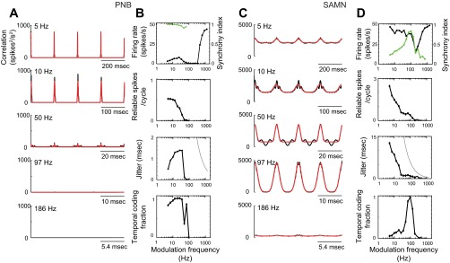
Spike-timing precision and reliability analysis for a single neuron [BF = 19.0 kHz, best modulation frequency (BMF) (PNB) = 26 Hz, BMF (SAMN) = 100 Hz]. A and C: shuffled correlograms for the single unit (black) are shown for PNB and SAMN, respectively, over a range of modulation frequencies (5, 10, 50, 186 Hz). The shuffled correlogram of the optimal (best-fit) neuron model is shown for each condition as a superimposed red curve. B and D, top to bottom: the rate modulation transfer function (black) for this neuron exhibited a predominant high-pass pattern for PNB and a notch response pattern for SAMN. The synchrony modulation transfer function (superimposed green curve) displayed low-pass pattern for PNB and band-pass pattern for SAMN. Synchrony data points with nonsignificant value are not plotted (Raleigh statistic, P < 0.001). By comparison, the spiking reliability transfer function (i.e., the number of temporally reliable spikes as a function of modulation frequency) demonstrates that spiking reliability decreases systematically with increasing modulation frequency. The spike-timing jitter transfer function for the select neuron shows how spike-timing jitter varies with the sound modulation frequency. For PNB (B), the unit exhibited low jitter (<2 ms), as observed for frequencies between 5 and 69 Hz, where the response was statistically significant (t-test, P < 0.05). For SAMN (D), the temporal precision decreased systematically with the sound modulation frequency. For reference, gray lines represent the expected estimated jitter for a Poisson neuron of identical spike rate (Avissar et al. 2007). B and D, bottom: temporal coding fraction transfer functions for the selected neuron are shown for PNB and SAMN, respectively. The temporal coding fraction represents the proportion of the spike train power that is attributed to reliable temporally phase-locked action potentials. For PNB, the temporal coding fraction exhibits a low-pass pattern indicating that reliable, temporally locked activity was present for low frequencies. By comparison, the temporal coding fraction of SAMN is tuned, indicating that reliable temporally locked activity was dominant within the vicinity of 100-Hz modulation frequency. Dots on the curves of B and D indicate significant results relative to a Poisson neuron with identical rate modulation transfer function (t-test, P < 0.05).
Finally, to quantify the fractional number of spikes that were reliably phase-locked to the stimulus, we computed the temporal coding fraction (F) as the ratio of phase-locked power to total power in the spike train:
| (5) |
where Φperiod(τ) represents the shuffled autocorrelogram of the periodic response component. As can be seen, this metric lies between 0 and 1, where 1 indicates that 100% of the action potentials are reliably phase-locked to the periodic sound.
Significance testing of the parameters was performed by considering a Poisson model of identical spike rate as a null hypothesis. The Poisson neuron assumption was chosen as a reference because the action potentials for such a neuron would be randomly distributed in the cycle histogram, and the autocorrelogram will not exhibit a synchronized peak (i.e., x̄ and F are both 0). The Poisson model was simulated and the data were bootstrapped to derive error bounds for the real data and the Poisson simulation. A t-test was then performed for the real data to test against the Poisson model at significance level of P < 0.05 for all parameters. Significant temporal synchrony was not observed beyond 500 Hz, and, therefore, data conditions beyond this range were not included in the present findings.
Model Validation
The quality of the model was assessed with a cross-validation procedure in which half of the neural data were used for model optimization, and the remaining half for model validation. To do this, the dot-rasters at each modulation condition were first subdivided into non-overlapping 4-cycle segments. Odd and even segments were used to compute independent shuffled correlograms that were used for model validation [Φ1(t)] and optimization [Φ2(t)], respectively. The validation procedure was performed for every neuron at all sound conditions (PNB and SAMN, multiple modulation frequencies) that yielded statistically significant synchrony (P < 0.05, as described in the previous paragraph). Because, as shown in the results section, the response properties of neurons (i.e., baseline firing rate, spike-timing jitter, firing reliability) can change substantially with the specific stimulus condition (e.g., PNB vs. SAMN, 5 Hz vs. 100 Hz), the validation procedure is not designed to assess how well the model generalizes across stimulus conditions. Instead, our intent is to use the model to derive meaningful parameters of the neural response (spike-timing jitter and reliability), which can then be used to characterize the relationship between a particular sound and the response pattern.
Two error metrics were defined to assess the quality of the model fits. First, we considered the fractional model error:
| (6) |
This error metric expresses the power of the difference signal as a percentage of the power of the empirical shuffled correlogram.
Because the neural data contain both deterministic model errors as well as measurement noise, we devised a second error metric that compensates for the measurement noise and strictly captures deterministic errors resulting from deviations in the model fits. The noise-corrected error metric was obtained as (appendix b):
| (7) |
Like the error metric of Eq. 6, this metric expresses the model error as a percentage of the total signal power; however, bias due to measurement noise is removed from the estimate (see appendix b). As expected, both metrics yield similar results, although the corrected error metric yielded slightly smaller estimates of the errors.
Information Theoretic Analysis
We consider how much information is contained by the temporal response pattern for each stimulus. Specifically, we are interested in identifying how spike-timing precision and firing reliability contribute to the representation of periodic stimuli with different shapes. To do this, we defined and computed the specific temporal information (STI) for each stimulus condition (i.e., the specific stimulus: modulation frequency, PNB, or SAMN) and determined how spike-timing reliability and jitter contribute to the information encoding efficiency using an information theoretic approach. Formally, it is shown that the total mutual information can be decomposed as (appendix c)
| (8) |
where ISTI(Wk, Sk) is the STI that is contained in the temporal response pattern for a specific stimulus-response ensemble (Sk, Wk). The second term IEI is the ensemble information (EI) that can be gained by comparing responses across the stimulus-responses ensembles. The decomposition of Eq. 8 is based on the assumption that both the stimuli and responses are conditionally independent (see appendix c). Here, the primary goal is to decipher how the stimulus information was carried by the temporal response pattern for each specific stimulus, and thus we will focus on characterizing the STI.
The STI was calculated using a model-based approach in which we simulated model spike trains fitted to the original data. We employed this approach because we can synthesize extended spike trains with a larger number response cycles, which is necessary to minimize bias in the information calculation (Strong et al. 1998). As shown in Fig. 2, the model spike trains closely resembled the original spike trains, both in terms of the deterministic response and the statistical structure. Hence the resulting STI trends were the same for the original data and model, although numerically smaller for the model spike trains (due to the reduced positive information bias; see Information bias correction).
Fig. 2.

Temporal reliability and spike-timing jitter analysis. A–C, middle panel: example neural response to PNB (A) and SAMN (B and C) at 10-Hz modulation frequency are shown as dot-rasters for three single neurons [A: best frequency (BF) = 17.5 kHz, B: BF = 4.8 kHz, C: BF = 20.7 kHz]. For reference, the top panel depicts the 400-ms segment of the corresponding PNB and SAMN sounds. Note that the vertical alignment of the action potentials (dots) is indicative of the precision of the spike arrival times (jitter). For PNB, the neural response is characterized by phasic periodic pattern, while for SAMN the action potentials are broadly distributed across the sound modulation cycles. A–C, bottom panel: dot-rasters for the proposed neural model that incorporates spike-timing and spiking reliability errors (see methods; appendix a) accurately replicates the observed neural response patterns. The best-fit model was obtained for each condition by finding the spiking reliability, spike-timing jitter, and baseline firing rate of the model that most closely matched the neural response. D–F: shuffled correlograms for the responses shown in A–C (black), respectively. The shuffled correlogram of the model is superimposed (red). G–J: summary data for the raw (G and I) and noise-corrected model errors (H and J; see methods; appendix c) are shown as box-whisker plots as function of sound condition [PNB (I and J) and SAMN (G and H), multiple modulation frequencies]. In all panels, errors are normalized as percentage of the total response power. The notches in the box designate the median errors, and the limits of the box determine the upper and lower quartile of the errors. Whiskers lengths are set to 1.5 times the interquartile range. Neurons that exceeded this range are shown as +. The model fitting was performed only for conditions with statistically significant firing reliability relative to a Poisson neuron of identical spike rate (P < 0.05, see methods).
Measuring STI.
Neural responses were first fitted to a spiking model with spike-timing jitter, reliability, and additive spontaneous firing using Eqs. 3 and 4. Simulated spike trains with 8,000 response cycles were then generated according to Eq. A2 for each stimulus condition, as illustrated in Fig. 2.
The STI was estimated from these model spike trains by adapting the procedure of Strong et al. (1998):
| (9) |
where HTotal(k) and HNoise(k) are the total and noise entropy, respectively, after conditioning on a specific stimulus-response ensembles (Sk, Wk). We will refer to these as the specific entropy and specific noise entropy, respectively. Note that for simplicity, we use the abbreviated notation ISTI(k) = ISTI(Sk, Wk).
The total specific entropy [HTotal(k)] was estimated by measuring the probability distribution of observing arbitrary B-bit words in the neural response (Strong et al. 1998):
| (10) |
Here, pk(w) = p(w|Sk, Wk)is the probability distribution of observing a particular word in the spike train conditioned on the specific stimulus-response ensemble. This distribution was estimated by subdividing the spike trains into overlapped B-bit words (w) containing 0 or 1 spike per bin using a fixed bin width of Δt = 1 ms. Since the goal is to measure the information that is available from the periodic temporal response pattern of PNB or SAMN, the response words were chosen as precisely one period duration (T = 1/fm), so that the number of bits per word increases with decreasing modulation frequency [B = T/Δt = 1/(Δt·fm)]. This is done because any temporal information will be reflected at the fundamental frequency of the stimulus or possibly in the higher-order harmonics that may arise from nonlinear distortions and which are reflected in a single response cycle.
Next we estimated the noise entropy associated with the response for the specific stimulus-response ensemble. In the approach proposed by Strong et al. (1998), the noise entropy is computed by considering the word entropy observed across response trials at a particular time, tj, and subsequently averaging across all time instants:
| (11) |
where 〈·〉 denotes a time average. Here, pk(w|tj) represents the probability of observing a B-bit word given the specific stimulus-response (Sk,Wk) and time instant (tj). For the case of the periodic spike trains obtained here, we employ a modified procedure in which we condition on the cycle phase (θj; as opposed to the a particular time instant, tj) because the deterministic features of the response are periodic and reoccur at all phases of the envelope [i.e., pk(w|θj) = pk(w|θj + 2π) in the original dot-raster]. That is, the response words are statistically identical if taken at a particular phase, regardless of the absolute time of occurrence. Thus, rather than conditioning on a particular time instant, we condition on the stimulus phase θj:
| (12) |
where the average operator 〈·〉 is performed across all the stimulus phases, θj. Here the phase is chosen at a sampling resolution θj = 2πj·Δt/T = 2πj/B, where j = 1, … , B, so that all temporal word configurations in the periodic response are considered. Note that at each phase the word distribution, pk(w|θj) is estimated directly from the cycle-dot raster (see Fig. 6). We have empirically verified the validity of this approach using simulated spike trains, and both the phase and time-averaging approaches produce identical results in the limiting case where the number of trials is large. Equation 12 is preferred over Eq. 11 because bias in the information calculation is largely attributed to the limited number of response trials (e.g., 10 trials for 200 Hz) (Strong et al. 1998). When using Eq. 11, there are substantially more cycles (e.g., 8,000 vs. 10, for the 200-Hz condition) because the approach considers all cycles taken across trials and time (e.g., 4 s/trial × 200 cycles/s × 10 trials = 8,000 cycles, for the 200-Hz condition), which substantially reduces the information bias.
Fig. 6.
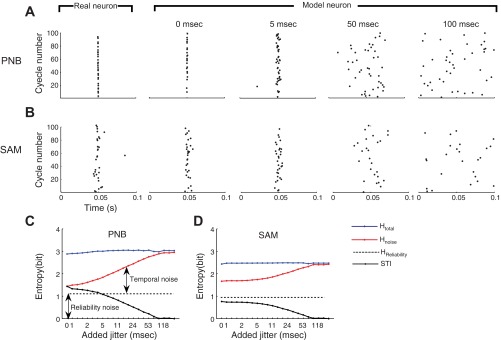
Specific temporal information (STI) analysis. Cycle dot-rasters are shown for a neuron (BF = 18.2 kHz) at 10-Hz modulation frequency (A and B, left panel) along with fitted model responses (A and B, second panel; 100 out of 8,000 simulated cycles are shown). For both PNB and SAMN, the neuron exhibits reliable and precisely timed responses (PNB, σ = 0.5 ms, x̄ = 0.31; SAMN, σ = 2.2 ms, x̄ = 0.27). For clarity of the following examples, the response delay has been removed from the dot-rasters so that the peak response occurs at 50 ms (for PNB and SAMN). The effective spike train temporal resolution of the model responses is varied by synthetically adding spike-timing jitter to the cycle dot-rasters (A and B, right panels; shown for 0, 5, 50, and 100 ms; see methods). C and D: the total specific entropy (Htotal; blue), specific noise entropy (Hnoise; red), and reliability noise entropy (dotted black), are shown as a function of the effective spike train resolution (i.e., added jitter; see methods). Note that the total specific entropy is relatively independent of the amount of added jitter, while the specific noise entropy increases with the amount of added jitter. The difference between the specific noise entropy (red) and the reliability noise entropy (dotted black) correspond to the temporal noise entropy (see methods). The STI associated with each stimulus (C and D, black) is obtained by subtracting the specific noise entropy from the total specific entropy and correcting for the measurement bias (see methods). For both SAMN and PNB, the STI decreases with increasing amount of added jitter, thus reflecting the uncertainty in the neural responses created by the added jitter.
Information bias correction.
Two approaches were employed to correct for bias in the STI calculation. The first consisted of employing the model-based approach to estimate STI from simulated responses with 8,000 response cycles, which substantially reduces the STI bias. This was particularly important for low-modulation frequencies, where the number of response cycles that could be measured from the neural responses is small, resulting in undersampled word distributions and, consequently, substantially higher bias. For instance, at 5-Hz modulation frequency, there is a total of 200 cycles (10 trials × 4 s/trial × 5 cycles/s) in the original data from which to estimate the noise entropy via Eq. 12. By comparison, at 200-Hz modulation frequency, there was a total of 8,000 cycles that could be used to estimate the noise entropy. Furthermore, the word size is larger for low-modulation frequencies, which further exacerbates the bias at low-modulation frequencies (e.g., B = 5 at 200 Hz vs. B = 200 at 5 Hz). Together, these two factors lead to a substantially larger bias at low-modulation frequencies, even though the sound duration was identically for all conditions.
To determine a suitable number of response cycles that would minimize the bias of the simulated model spike trains, we first generated simulated model spike trains according to Eq. A2, with a variable number of response cycles (500, 1,000, 2,000, 4,000, 8,000). The spike trains were optimized to match the temporal response pattern for each condition, as outlined in Eqs. 3 and 4 and shown in Fig. 2. The measured information dropped off with increasing number of cycles due to decreasing bias. For 8,000 cycles, the residual bias was small (<10%), and thus the STI was calculated using the 8,000 cycles condition.
To further correct for unaccounted residual bias, we subtracted the measured STI for a random Poisson neuron of equal spike rate: ĪSTI(k) = ISTI(k) − IResBias(k). We refer to this quantity as the residual bias [IResBias(k)]. Note that, ideally, STI is zero for the response of a Poisson neuron that fires independently from trial to trial in response to the periodic sounds. However, due to limitations in the information calculation and data size, the measured information for the Poisson spike train was found to be greater than zero. When tested across data sizes (500, 1,000, 2,000, 4,000, 8,000 cycles), the trend for the reduction in this residual bias with increasing data size was nearly identical to that observed for reductions in the STI, indicating that the residual bias for a Poisson condition accounts for the bias in the simulated data at multiple conditions. For the 8,000 cycles simulations, the mean residual bias was small at 2.8% and 3.0% for PNB and SAM, respectively.
Temporal Noise Entropy, Reliability Noise Entropy, and Coding Efficiency
To characterize how spike-count reliability and spike-timing jitter affect the encoding and temporal information transfer of CNIC neurons, the specific noise entropy was decomposed by considering the fractional entropy that resulted from reliability and spike-timing noise. Consider a framework in which a noiseless neuron produces a perfectly reproducible response for each modulation cycle. The neural spike train and the corresponding B-bit words for the noiseless neuron are perfectly reproducible across cycles so that the noise entropy would be precisely 0 bits because there is no variability from cycle to cycle in the response words. For a real neuron, the cycle-to-cycle spike train variability could result from either spike-count variability or spike-timing errors. For a specific stimulus-response ensemble, the specific noise entropy reflects these two forms of variability and thus can be decomposed as HNoise(k) = Htemporal(k) + Hreliability(k) (appendix d), where the reliability noise entropy [Hreliability(k)] strictly arises from spike-count reliability errors, and the temporal noise entropy [Htemporal(k)] arises from spike-timing errors. For simplicity, we assume that the specific stimulus is implied throughout and will use the abbreviated notation HNoise = Htemporal + Hreliability.
The reliability noise entropy is defined as the entropy that strictly arises from deviations in the spike count from cycle to cycle. That is, it reflects only variability due to spike-count reliability errors across cycles independently of spike-timing errors. It is computed as the entropy of the spike count distribution, which reflects cycle-to-cycle variability not due to spike-timing errors (appendix d, Eq. D6). In contrast, the temporal noise entropy strictly arises from spike-timing errors and is formally derived from the conditional response word distribution when the spike count is fixed (appendix d, Eqs. D4 and D5):
| (13a) |
| (13b) |
where L is the subset of words with precisely l spikes, pNoise(w | l) is the word distribution conditioned for l spikes, Htemporal(l) corresponds to the specific temporal entropy when the spike count is fixed, and Htemporal is the average specific temporal entropy (averaged across all spike counts).
To quantify the contribution of spike-timing jitter and spiking reliability in the neural response and to characterize how these forms of noise depend on the sound period and envelope shape, we consider the fraction of the noise entropy that results from reliability or spike-timing errors for a specific stimulus. The reliability noise fraction and temporal noise fraction are defined as the proportion of the total spike train entropy that could be accounted for by reliability or spike-timing errors:
| (14) |
and
| (15) |
Note that the reliability and temporal noise fractions both depend on the temporal analysis resolution. Furthermore, the proportion of specific noise entropy in the response (i.e., the noise fraction) is simply the sum of the reliability and temporal noise fractions:
| (16) |
Based on the definition of coding efficiency (Rieke et al. 1995), it is easy to show that these quantities are intimately related to the specific temporal coding efficiency of the neuron according to the following relationship:
| (17) |
Thus the temporal encoding efficiency decreases as either the reliability or temporal noise fraction increases.
Efficiency and Spike-timing Resolution
We also determined how encoding efficiency depend on the resolution of the neural spike train. To do this, we varied the effective spike train resolution by synthetically adding spike-timing jitter (see Fig. 6) to the neural spike trains prior to computing the STI, efficiency, and noise fractions. This procedure is analogous to that employed previously to determine the role of precise spike timing (Kayser et al. 2010; Lu and Wang 2004). Information metrics were calculated for each sound condition using different amounts of added spike-timing jitter (uniformly distributed, 1- to 200-ms range, in 0.38 octave steps). This procedure is used to characterize how temporal resolution affects encoding efficiency for both PNB and SAM.
RESULTS
We examined how envelope periodicity and shape cues influence spike-timing precision and reliability and how these factors influence information transmission in the cat CNIC. Specifically, we hypothesized that the envelope shape and period will systematically affect the spike-timing precision and reliability so that these temporal response attributes can potentially convey substantial stimulus information. Data consist of 65 single units that were driven with PNB and SAMN (Fig. 1, top; shown for 5, 7, and 10 Hz). Both sounds span identical modulation frequencies; however, their envelope shapes are distinctly different. Specifically, although the period of the PNB can be changed by adjusting the modulation frequency parameter, the shape of the envelope (i.e., the attack and decay times) is constant for all modulation conditions (Fig. 1, bottom left; consisting of a brief 250-μs pulse). Thus differences in neural firing pattern for different PNB modulation frequencies will strictly reflect changes in the period of the sound. In contrast, the envelope shape for SAMN covaries with the sound modulation frequency so that both acoustic attributes can theoretically affect the neural response (Fig. 1, bottom right). For low-modulation frequencies, the envelopes exhibit slow attack and decay times, and these become faster with increasing modulation frequency. These stimulus conditions thus allow us to parse out how pure repetition (PNB) or combined repetition and shape cues (SAMN) are concurrently encoded (Zheng and Escabí 2008).
Fig. 1.

Acoustic stimuli. Periodic noise bursts (PNB) and sinusoidal amplitude modulated noise (SAMN) were delivered at multiple modulation frequencies (5, 7, and 10 Hz are shown; top panels). The stimulus envelope (middle panels) is superimposed for 5, 7, and 10 Hz (blue, red, and green, respectively). Although for PNB the envelope shape is constant for all modulation frequencies (bottom left), this is not the case for SAMN (bottom right). The envelope shape for SAMN covaries with the modulation frequency, since higher modulation frequency sounds have faster rise and decay times.
The temporal structure of the neural responses to periodic stimuli was strongly dependent on the envelope shape. Example responses are illustrated for three units as 400-ms dot-raster segments for 10-Hz modulation frequency (Fig. 2, A–C, middle panel). As previously demonstrated, the neural responses exhibit distinct discharge patterns for PNB and SAMN that are complementary to the shape of the envelope waveform (Zheng and Escabí 2008). First, units often displayed precisely phase-locked response to the brief noise burst of the PNB, as evidenced by the tightly alignment episodes in the dot-rasters (Fig. 2A, middle panel) and the sharp events in the shuffled correlogram of a single neuron (Fig. 2D). Second, the SAMN spike trains are often more variable, although the spiking pattern accurately reflects the envelope structure of the sound (Fig. 2, B and C, middle panel). This behavior is seen in the response shuffled correlogram, which displays a temporally broad periodic pattern that closely mimics the SAMN stimulus envelope as seen from the shuffled autocorrelograms (Fig. 2E, F).
The Contribution of Envelope Periodicity and Shape to Spiking Reliability and Precision
The example response patterns of Fig. 2 demonstrate that neurons can encode the sound envelope waveform by their precise discharge pattern. Neural precision clearly varies for the example units; however, the factors that govern precision and reliability of neural spiking in the CNIC are unknown. One possibility is that spiking precision and reliability strictly reflect intrinsic properties of the neuron, such as its membrane time constant, refractory period, or the synaptic variability. For this scenario, it is expected that precision and reliability are largely stimulus independent, because precision and reliability would be dominated by the neuron's biophysical properties. Alternately, it is also possible that spiking precision and reliability are strongly influenced by the stimulus characteristics. Specifically, although it is generally assumed that periodicity is the primary acoustic factor affecting temporal response properties, we hypothesize that the envelope waveform shape strongly influences the unit spiking properties. As illustrated in Fig. 2, A–C, the discharge spike-timing precision (jitter) for the select neurons appear to depend on the stimulus condition. Responses to PNB are typically characterized by precisely phase-locked action potentials, while the discharge patterns to SAMN at identical modulation frequency lack precisely phase-locked spikes, and the firing pattern appears to reflect the envelope shape. These differences suggest that the stimulus envelope shape and period may independently influence the precision and reliability of firing.
We first characterized how shape and periodicity influence spike-timing precision and firing reliability. To do this, we developed a stochastic neural model that incorporates three forms of spiking noise seen in vivo: spike-timing jitter, spiking reliability, and random asynchronous spikes (see methods and appendix). Dot-rasters from the model fits to the neural data are shown in Fig. 2, A–C (bottom, red dot-rasters). Visually, the model replicates the temporal response pattern quite well. For each unit and stimulus condition, we first computed the shuffled correlogram and developed a closed-form solution for the shuffled correlogram of the spiking model under the assumption of normally distributed spike-timing jitter (methods, Eq. 3). The model parameters (jitter, number of reliable spikes, and baseline firing rate) were iteratively optimized to find the model configuration that most closely resembled the neural data (see methods). Shuffled correlogram model fits are illustrated for the examples of Fig. 2, D–F (superimposed red curve). Consistent with the model dot-rasters, the predicted shuffled correlograms provide a good approximation to the neural data (1.7%, 1.1%, and 0.1% error for A, B, and C; chi-square test, P < 0.05). Summary statistics for the raw and noise-corrected model errors (see methods) are shown as box-plots for SAMN (Fig. 2, G and H) and PNB (Fig. 2, I and J) at multiple modulation conditions. As can be seen, the noise-corrected errors are small for the majority of neurons and conditions, implying that the model accurately fits the neural data (SAMN median < 2%, PNB < 10% for most conditions).
Spiking reliability and precision were strongly dependent on the stimulus condition, as shown for an example CNIC neuron (Fig. 3). Shuffled correlograms are shown for a single neuron at different repetition rates for PNB (Fig. 3A, black) and SAMN (Fig. 3C, black) along with the model fits (red). The shuffled correlograms for PNB are characterized by a narrow peak at zero lag and at intervals corresponding to the stimulus period (Fig. 3A). As can be seen, the unit exhibited precise time-locking to the stimulus (∼1-ms resolution) over a wide range of modulation frequencies. For SAMN, the shuffled correlograms were generally much broader and lacked the high temporal precision observed for PNB (Fig. 3C). Furthermore, while the temporal spiking precision was relatively fixed for PNB, it was much more variable for SAMN. Note that the width of the correlogram peaks for SAMN become progressively narrower with increasing modulation frequency.
The relationship between firing reliability and spike-timing jitter for the example neuron exhibited distinct trends for PNB and SAMN (Fig. 3, B and D). First, spike-timing jitter was exceedingly small for PNB (<2 ms; Fig. 3B, third panel) for all modulation frequencies that produced significant results (5–69 Hz; tested against a Poisson neuron of identical firing rate, t-test, P < 0.05). In contrast, spike-timing jitter was substantially larger (up to ∼13 ms) and decreased systematically with increasing modulation frequency for SAMN (Fig. 3D, third panel). Although the neuron exhibited a high-pass rate modulation transfer function pattern for PNB and a notch rate modulation transfer function pattern for SAMN (Fig. 3, B and D, top), the number of reliable spikes exhibited consistent patterns with modulation frequency (Fig. 3, B and D; second panel). The number of reliable spikes is roughly flat (∼0.5 spikes/cycle) up to around 20 Hz for PNB and decreases systematically with increasing modulation frequency. Similarly, for SAMN, the number of reliable spikes decreased systematically with increasing modulation frequency. Finally, the temporal coding fraction quantifies the fractional power in the neural response that is phase-locked to the stimulus envelope and which potentially conveys temporal information (see methods). For this unit, the temporal coding fraction for PNB was close to 1 below 97-Hz modulation frequency (Fig. 3B, bottom), indicating that close to 100% of the action potentials were phase-locked to the sound and contributed to the temporal information within this range of modulation frequencies. In contrast, the temporal coding fraction for SAMN exhibited a band-pass behavior for this unit with a maximum at ∼100 Hz (Fig. 3D, bottom).
Spike-timing jitter and reliability for SAMN and PNB exhibited distinct trends across our population of units. First, there was not a strong dependence between jitter and reliability for PNB as evident by the lack of correlation between these parameters (Fig. 4A; r = −0.1 ± 0.05, nonsignificant). The scatter plot is clustered at fine temporal precision with most jitter values below 1 ms. For most modulation frequencies and units, the number of reliable spikes per stimulus rarely exceeded 1 spike/stimulus (average = 0.36 spikes/stimulus between 5- and 259-Hz modulation frequency), suggesting that the PNB envelope is explicitly represented by precisely phase-locked unitary action potentials. Furthermore, average firing rates are relatively independent of modulation frequency (Fig. 5A, red) and were weakly related to the firing reliability (r = 0.22 ± 0.48, mean ± SD). In contrast, the response synchrony exhibited a low-pass pattern (Fig. 5B, red). Both the average spiking reliability (Fig. 5C, red) and temporal coding fraction (Fig. 5D, red) exhibited a low-pass trend for PNB with modulation frequency. This is consistent with the idea that a low-pass filtering mechanism limits the amount of temporal phase-locking to the stimulus envelope. Furthermore, unlike spiking reliability, the average spike-timing jitter was small and relatively constant (∼300 μs) across modulation frequencies for PNB (5–259 Hz) (Fig. 5E, red, bootstrap t-test, P < 0.05). Thus the temporal coding precision for PNB does not depend strongly on the sound modulation frequency and is likely more influenced by the constant envelope shape.
Fig. 4.

Relationship between spike-timing precision and reliability and their dependence on the envelope shape and modulation frequency. A: spike-timing precision (jitter) was largely independent of the stimulus condition for PNB, whereas firing reliability decreased systematically with repetition (P < 0.05). Each data point (triangle) represents a single neuron at the specified repetition condition (5, 10, 19, 36, 69, 134 Hz). Only neurons for which the spiking reliability was significant at a specific condition are shown (P < 0.05). The population averaged reliability and jitter (circles) and the corresponding standard deviation (vertical and horizontal bars) are shown for each condition. B: for SAMN, spiking reliability and jitter were strongly correlated (Pearson's r = 0.65 ± 0.05, P < 0.01). Jitter and reliability were highly clustered for each condition and both systematically increase with decreasing modulation frequency.
Fig. 5.

Population response trends. A: the average normalized firing rate across neurons is shown as a function modulation frequency for SAMN (black) and PNB (red). For both SAMN and PNB, firing rates are relatively independent of modulation frequency. B: the response synchrony exhibits a low-pass trend for PNB. For SAMN, the overall synchrony is lower and exhibits a band-pass pattern across the neural population. C: the average reliability decreases monotonically with increasing modulation frequency for both SAMN and PNB. D: a similar low-pass trend is observed for the mean temporal coding fraction (i.e., the proportion of the spike train power that is phase locked to the sound), indicating that phase-locked activity contributes most for low frequencies. E: for SAMN, the mean spike-timing jitter decreased systematically with increasing modulation frequency. In contrast, for PNB, the mean spike-timing jitter was small (∼300 μs) and relatively constant for modulation frequencies below 200 Hz (inset shows for PNB). Gray line indicates the theoretical spike-timing jitter that would be measured for a Poisson neuron (Avissar et al. 2007). Error bars indicate standard error of the mean.
In contrast to the highly stereotyped PNB response pattern, the SAMN response pattern was more varied across modulation frequencies. For each condition, the spike-timing jitter and the number of reliable spikes for different units were strongly clustered for different modulation frequencies (Fig. 4B). The clustering of these response parameters was strongly dependent on the modulation condition, leading to a strong correlation between jitter and reliability (r = 0.65 ± 0.05, mean ± SD; P < 0.01). Spike rates were relatively constant across modulation frequencies (Fig. 5A, black) and were weakly related to the firing reliability (r = 0.35 ± 0.41; mean ± SD). The average vector strengths (VS) exhibited a band-pass trend (Fig. 5B, black) for SAMN and was also weakly correlated with the spike-timing jitter (r = 0.22 ± 0.35; mean ± SD). Similar to PNB, the average reliability (Fig. 5C, black) and the temporal coding fraction (Fig. 5D, black) decreased with increasing modulation frequency. Although the firing reliability and temporal coding fraction trends exhibit a similar low-pass filter behavior for SAMN and PNB, the average number of reliable spikes was on average higher and temporal coding fraction was lower for SAMN. This suggests that SAMN tended to produce on average more phase-locked action potentials (higher number of reliable spikes) to the stimulus envelope compared with PNB, although these were accompanied by a higher level of undriven random firing (thus the lower temporal coding fraction). Furthermore, unlike for PNB where the spike-timing jitter was roughly constant with modulation frequency (Fig. 5E, red), spike-timing jitter decreased systematically with increasing modulation frequency for SAMN (Fig. 5E, black).
Overall, the systematic and highly consistent relationship between envelope shape and jitter and modulation frequency and firing reliability support the hypothesis that spike-timing jitter is strongly influenced by the envelope shape of the sound, whereas spiking reliability is much more affected by the sound period (see discussion).
Specific Temporal Information
The highly consistent trends observed in the correlogram analysis demonstrate that spike-timing precision and reliability can potentially encode the shape and repetition of acoustic envelopes, respectively. This raises several questions regarding the structure of the neural code in the CNIC. First, it is of interest to determine how much information is carried by the temporal signature of the neural response for a specific stimulus. Second, as demonstrated, response variability in the form of spike-timing jitter and firing reliability vary systematically with the stimulus parameters (shape and modulation frequency), and these in turn affect the information transfer. Thus it would be of interest to determine how the sound periodicity and envelope shape contribute to the temporal information transfer of the neuron.
The procedure for measuring the STI from neural responses is illustrated in Fig. 6 (see methods). The STI was designed to quantify the available information from the periodic temporal response pattern to a “specific” sound. It is estimated with a model-based approach in which the neural response were fitted to the model (as in Fig. 2) and synthetic spike trains were generated with large number of response cycles to minimize measurement bias (8,000 simulated cycles; see methods). To examine the effects of spike-timing resolution on STI, we varied the effective spike train resolution by synthetically adding spike-timing jitter to the model spike trains (1–200 ms in 0.38 octave steps) (Kayser et al. 2010; Lu and Wang 2004). Cycle dot-rasters from a single neuron are shown for PNB (Fig. 6A) and SAMN (Fig. 6B) at 10-Hz modulation frequency, along with model spike trains with varying amounts of added spike-timing jitter (Fig. 6, A and B: 0, 5, 50, 100 ms). For both sounds (PNB and SAMN at 10 Hz), the total spike train entropy (specific entropy) was relatively constant for multiple analysis spike train resolutions (Fig. 6, C and D, blue curve). However, the specific noise entropy increases with decreasing spike train resolution (Fig. 6, C and D, red curve) because the added spike-timing jitter adds spike-timing variability to the neural spike train. The STI is obtained by subtracting the specific noise entropy from the specific total entropy and correcting for bias in the measurement (Fig. 6, C and D, black curve; see methods). Note that, when the analysis spike train resolution roughly corresponds to or exceeds one period of the stimulus (i.e., 100 ms for this example), the specific entropy and specific noise entropy are equal and the STI is precisely zero. This occurs because, when the added spike-timing jitter is equal to or greater than the cycle period, the spike-timing patterns are completely randomized, and there is no consistent firing pattern across stimulus trials.
Several distinct trends were observed in the neural activity that reflected the SAMN and PNB stimulus structure. First, the measured STI on a per-cycle basis (bits/cycle) decreases systematically with increasing modulation frequency for both PNB and SAM. This behavior is seen for individual examples (Fig. 7, A and B, left panels), as well as the neural population (Fig. 7C, left panel). Furthermore, for the examples and population, the magnitude of the STI is larger for PNB (bootstrap t-test with Bonferroni correction, P < 0.05 for 5–134 Hz), consistent with the fact that temporal responses are more precise for PNB (Fig. 5E) and thus can convey more stimulus information through precise spike timing. The decreasing trend with modulation frequency is largely attributed to the fact that temporal reliability decreases with increasing modulation frequency for both PNB and SAMN (Fig. 5C). By comparison, when we measured the available STI per unit time (i.e., the STI rate; bits/s), a distinctly different picture is obtained. For both PNB and SAMN, the temporal information that is conveyed on average could be tuned for individual neurons (Fig. 7, A and B, right panel) and tended to be larger in magnitude for PNB compared with SAMN. Likewise, for the neural population, the STI rate was tuned as a function of modulation frequency (Fig. 7C, right panel) and larger for PNB (bootstrap t-test with Bonferroni correction, P < 0.05 from 5–134 Hz). The STI rate peaked at 97-Hz modulation frequency for PNB (19 bits/s maximum, red) with an upper limit of ∼200 Hz (half-maximum between 186 and 259 Hz), while for SAMN the STI rate was substantially lower (6 bits/s maximum) with a peak around 26 Hz and an upper limit of ∼100 Hz (50% amplitude relative to the peak at ∼97 Hz, black). Thus, although the available information per cycle decreases with modulation frequency, as a consequence of unreliable firing, substantial stimulus information can be accumulated over time. This occurs because, although the STI per cycles is high at low-modulation frequencies, there are relatively few cycles for which to accumulate temporal information (e.g., 5 cycles over 1 s at 5 Hz). In contrast, substantial temporal information can be gained for high-modulation frequencies by observing responses over time, even though the STI conveyed by one cycle is relatively small. This is particularly true for PNB, where the precise spike timing to the transient PNB envelopes leads to higher information per cycle, and, in turn, temporal information can be conveyed up to ∼200 Hz. As proposed below, such differences in the STI rate pattern for PNB and SAMN reflect differences in the neural response that are associated with the sound envelope shape.
Fig. 7.

STI dependence with modulation frequency and envelope shape. The STI is shown for two neurons (A and B) as a function of modulation frequency for SAMN (black) and PNB (red). For both example unit I (BF = 1.9 kHz; A) and II (BF = 40.8 kHz; B), the STI (in bits/cycle) decreases systematically with increasing modulation frequency for SAMN and PNB, although it was larger in magnitude for PNB. By comparison, the STI rate (STI per unit time; bits/s) is tuned for both SAMN and PNB and is likewise larger for PNB. C: similar behavior is seen in the population average results (error bars indicate SEM).
The Contribution of Spike-timing Jitter and Reliability on Temporal Coding Efficiency
As demonstrated, the period and envelope shape of SAMN and PNB have a pronounced effect on the temporal precision and reliability of neural responses. These systematic differences ultimately influence the temporal information transfer of CNIC neurons. Here we examine how these acoustic (shape and periodicity) and neuronal response (jitter and reliability) factors separately influence the coding efficiency.
The coding efficiency of a neuron is defined as the fraction of the total spike train entropy that contains stimulus-related information (Rieke et al. 1995). Noting that spiking noise limits stimulus information transfer, we, therefore, characterized how spike-timing jitter and reliability errors contribute to the temporal coding efficiency. To do this, we consider the fraction of the total entropy that could be attributed to reliability and spike-timing errors (see methods). The temporal (Ftemporal) and reliability (Freliability) noise fractions were defined as the fraction of the total entropy that was attributed to spike-timing (jitter) or spiking reliability errors. The temporal coding efficiency is then E = 1 − Freliability − Ftemporal (see methods and appendix d). Figure 8, A and B (left panels), shows the temporal coding efficiency trends from two single neurons. For both PNB and SAMN, the temporal coding efficiency decreases systematically with the sound modulation frequency, although it tends to be somewhat higher for the PNB sound.
Fig. 8.

Relationship between temporal coding efficiency, temporal noise fraction, and reliability noise fractions. A and B, left panel: the temporal coding efficiency is shown for SAMN and PNB for two neurons (same neurons as in Fig. 7). For both examples, temporal coding efficiency decreases systematically with increasing modulation frequency for both SAMN and PNB, although the efficiency is higher for PNB. A and B: in contrast, the proportion of noise due to reliability errors (reliability noise fraction, middle panels) increases systematically with modulation frequency and is roughly equal in magnitude for SAMN and PNB. A and B: the proportion of noise attributed to spike-timing errors (temporal noise fraction, right panels), by comparison, decreases with modulation frequency and is larger in magnitude for SAMN. C: similar behavior is observed for the average population results (error bars indicate SEM).
For each unit, we decomposed the temporal coding efficiency into the reliability and temporal noise fractions and plotted these as a function modulation frequency (Fig. 8, A and B, middle and right panels). The reliability and temporal noise fractions represent the proportion of the total entropy that can be accounted by reliability and spike-timing errors, respectively (see methods and appendix d). Two distinct trends are observed. First, the reliability noise fraction for the select neurons exhibited similar trends for SAMN and PNB, where it tends to increase systematically with increasing modulation frequency (Fig. 8, A and B, middle panels). Thus the response entropy associated with reliability noise is lowest at low-modulation frequencies and tends to dominate at high-modulation frequencies. This is consistent with the measured reliability trends in which firing reliability decreases with modulation frequency (Fig. 5C). By comparison, the temporal noise fraction tends to decrease with modulation frequency and is lower in magnitude for PNB. The lower noise fraction observed for PNB reflects the fact that spike-timing noise is lower for PNB as a result of the higher spike-timing precision (Fig. 5E) and the proportion of temporally phase-locked spikes is higher for PNB (Fig. 5D).
Similar behavior is seen in the population trends (Fig. 8C). As for the example single neurons, the temporal coding efficiency decreases with increasing modulation frequency, and the overall magnitude was higher for PNB compared with SAMN (bootstrap t-test with Bonferroni correction, P < 0.05 from 5–259 Hz), indicating a higher signal-to-noise ratio for PNB. Interestingly, the reliability noise fraction trend was identical for PNB and SAMN (Fig. 8C, middle panel, bootstrap t-test with Bonferroni correction, nonsignificant), indicating that an equal proportion of the total response entropy could be accounted by reliability errors for both SAM and PNB. The reliability noise fraction increases systematically with increasing modulation frequency, reflecting the fact that firing reliability decreases with increasing modulation frequency (Fig. 5C). The similarity in the reliability trend for SAMN and PNB is consistent with the fact that spiking reliability depends primarily on the sound repetition, which is identical for both sounds. By comparison, the temporal noise fraction decreases with modulation frequency and is lower for PNB (Fig. 8C, right panel) (bootstrap t-test with Bonferroni correction, P < 0.05 from 5–360 Hz). This is consistent with the observation that spike-timing jitter and hence the amount of noise attributed to spike-timing errors is smaller for PNB compared with SAMN (Fig. 5E). Together, these findings indicate that the reduced temporal coding efficiency for SAMN (relative to PNB) is largely attributed to larger proportion of spike-timing noise for SAMN.
Since the primary acoustic difference between PNB and SAMN is the envelope shape, we hypothesize that observed disparity in temporal coding efficiency can be attributed to spike-timing differences arising from differences in the envelope shape. As demonstrated, the fractional response entropy attributed to spike-timing noise is larger for SAMN compared with PNB, which could reflect the sharper envelope (Fig. 1) and the resulting higher spike-timing precision for PNB (compared with SAM; Fig. 5E). By comparison, the fractional entropy attributed to reliability noise is identical for both PNB and SAMN (Fig. 8), likely reflecting the common periodicity for both sounds. Thus we expect that SAMN responses have coarser spike-timing precision, which ultimately increases the temporal noise entropy and thus reduces the overall temporal coding efficiency. To test for this possibility, we varied the effective temporal resolution of the PNB and SAMN responses by adding synthetic spike-timing jitter (as in Fig. 6, A and B) [Kayser et al. 2010 (no. 7041); Lu and Wang 2004 (no. 2186)] prior to computing the STI and temporal coding efficiency. As seen from selected examples (Fig. 6) and all other neurons tested, systematically adding spike-timing jitter to the neural responses produces a systematic reduction in the STI. This behavior is evident in the population average results since the STI decreases systematically with increasing spike-timing jitter for all modulation frequencies (Fig. 9, A and B). When the added spike-timing jitter is equal to or exceeds the modulation period, the temporal pattern of the response is completely randomized, and, consequently, no temporal information is available (the STI zero).
Fig. 9.

Relationship between the effective spike train resolution, STI, and temporal coding efficiency. Population average results showing how the effective spike train temporal resolution contributes to the STI (A and B) and temporal coding efficiency (C and D). The effective spike train temporal resolution was adjusted by adding synthetic spike-timing jitter (added jitter; as in Fig. 6) to the neural spike trains. As seen for both PNB (B and D) and SAMN (A and C), the average STI (A and B) and temporal coding efficiency (C and D) decrease with increasing added jitter for both PNB and SAMN. Furthermore, both the average STI and temporal coding efficiency were larger in magnitude for PNB (compared to SAMN). The dashed black contour in D corresponds to the equivalent spike train resolution, where the temporal coding efficiency of PNB matches that of SAMN with zero added jitter (dashed black contour in C). Note that the equivalent PNB spike train resolution (dashed black contour, D) follows the modulation period (gray contours, D) for each modulation frequency. E: histogram showing the equivalent PNB spike-timing resolution as a fraction of the modulation period (ratio of black to gray contour in D). The equivalent PNB spike train resolution required to match the SAMN efficiency is roughly a constant proportion of the modulation period (mean = 31%).
Given that PNB responses exhibit higher efficiency than SAMN and that reliability noise fraction is identical for both sounds (Fig. 8C), we asked whether the primary differences between PNB and SAMN responses could be accounted by differences in spike-timing resolution. To test for this possibility, we measured the equivalent PNB spike-timing resolution that is required to achieve comparable efficiency as SAMN (at each modulation frequency). That is, we added synthetic spike-timing jitter to the PNB responses until the efficiency of PNB at each modulation frequency was matched to the SAMN efficiency with zero-added spike-timing jitter (dashed black contour, Fig. 9C). The population average SAMN and PNB efficiencies are shown in Fig. 9, C and D, respectively, along with the matched efficiency contours for SAMN and PNB (Fig. 9, C and D; dashed black contours). As can be seen, adding spike-timing jitter to both PNB and SAMN responses reduces the temporal coding efficiency. Interestingly, the added PNB spike-timing jitter required to match the SAMN temporal coding efficiency with zero added jitter (dashed black contour) closely follows the modulation period (gray curve). On average, the added PNB spike-timing jitter required to match the SAMN efficiency corresponded to 31% of the modulation period (Fig. 9E). Thus PNB response can be synthetically modified to resemble SAMN responses by adding spike-timing jitter that is roughly a constant proportion of the modulation period. This result mirrors and is consistent with the fact that spike-timing jitter was small and independent of the modulation frequency for PNB while it covaried proportional to the time scale of envelope shape for SAMN (Fig. 5E).
DISCUSSION
Current theories of amplitude modulation coding aim to account for aspects of pitch and rhythm perception associated with the periodic structure of a sound. With few exceptions (Lu et al. 2001; Neuert et al. 2001; Pressnitzer et al. 2000; Zheng and Escabí 2008), most studies do not account for relevant loudness and timbre cues associated with the envelope shape of a sound (Irino and Patterson 1996). As demonstrated, the firing reliability and spike-timing precision were strongly affected by the sound period and shape in a manner that reflected the sound structure. Spike-timing precision covaried with the sound envelope shape, while the firing reliability was strongly dependent on, and decreased systematically with, increasing modulation frequency. These trends were closely tied and influenced the temporal information transfer and temporal coding efficiency. These results thus outline an encoding strategy in which the temporal firing pattern of CNIC neurons could simultaneously and efficiently represent periodicity and shape temporal cues.
The Role of Spike-timing Precision and Firing Reliability
The proposed framework employs the concept of spike-timing precision and firing reliability for studying the neural representation of shape and periodicity. Because firing reliability and spike-timing precision are essentially separate forms of variability in the temporal response pattern, our results demonstrate that neural “noise” or variability are inherently dependent on the sound structure. This brings up the possibility that spiking noise itself is an integral component of the neural code (Stein et al. 2005). Specifically, the observed dependence between temporal acoustic structure, reliability, and spike-timing noise could provide a means of signaling shape and periodicity-based cues.
Although firing rates were not systematically related to the sound shape or period, both jitter and reliability exhibited highly consistent response patterns from neuron to neuron, thus providing a robust signal to encode the acoustic envelope structure. For both SAMN and PNB, firing reliability was primarily affected by the sound period, while firing precision was strongly affected by the envelope shape. Firing reliability and the fraction of temporally locked action potentials decreased systematically with increasing modulation frequency. The decreasing nature of these trends may arise because of cell membrane and synaptic low-pass filtering which would limit temporal synchronization to all of the stimulus cycles with increasing modulation frequency (Geis and Borst 2009). Functionally, this trend could be related to the fact that pitch saliency degrades with increasing modulation frequency (Burns and Viemeister 1976). By comparison, firing precision was roughly constant for PNB at all modulation frequencies, although it varied systematically with the changing shape of the sound for SAMN.
The fact that central auditory neurons can respond with remarkable high temporal precision seems to be at odds with the fact that they cannot follow fast temporal modulations. Even within the auditory cortex, neurons can exhibit millisecond temporal firing precision to transient sound events, yet their ability to follow temporal modulations breaks down at ∼20 Hz (Elhilali et al. 2004; Heil and Irvine 1997; Joris et al. 2004). A similar dichotomy is evident in our data since neurons did not effectively follow temporal modulations beyond 300 Hz, although they could phase-lock with microsecond precision for PNB. We propose that this apparent dichotomy is related to separate encoding mechanisms. As demonstrated, spike-timing precision is strongly affected by the envelope shape of the sound. In contrast, the limiting ability to follow fast temporal modulations is related to the observed reduction in firing reliability with increasing modulation frequency. Thus our results may provide an explanation for this apparent paradoxical behavior on the basis of distinct response attributes and acoustic cues.
The proposed framework offers several advantages over other conventional approaches used to study temporal coding. Traditionally, the VS is used to quantify the precision of firing (Goldberg and Brown 1969). Despite its utility, the VS does not distinguish reliability from timing errors in the response pattern and strictly quantifies relative spike-timing precision (i.e., the proportional width of the cycle histogram). By comparison, the proposed jitter metric measures the absolute precision of firing (in ms). The correlation index proposed by Joris and colleagues (2006) has some appeal over VS; however, this metric depends both on reliability and precision of the responses. Given that reliability and precision are uniquely different forms of neural variability and, as shown here, can vary independently for different sound cues, the proposed reliability and spike-timing metrics should be of high appeal, because they can decompose and independently quantify these forms of neural variability. Furthermore, although not demonstrated here, the proposed framework and shuffled correlogram approach for measuring reliability and precision can be extended to the more general case of aperiodic signals (Chen and Escabí 2010).
The role of firing reliability and precision has been shown to be relevant in auditory structures outside the midbrain. In the AN, firing reliability and spike-timing precision decrease with increasing characteristic frequency for low-frequency tones (Avissar et al. 2007), analogous to our results for SAMN. Similar trends for reliable firing have also been described in the auditory cortex of awake primates (Malone et al. 2007). Collectively, these studies support the view that firing reliability and spike-timing precision could provide an alternative and more general framework to study the neural representation of temporal sound information.
Proportional vs. Absolute Spike-timing Precision
As demonstrated, CNIC neurons can generate spikes with extraordinary temporal precision (on the order of hundreds of microseconds), assuming that the sound structure is itself sufficiently precise. This result may seem somewhat trivial, given that the first-spike timing precision of neurons in the auditory system has been shown to be contingent on the shape of the rising envelope of a sound (Heil 1997b, 2001; Heil and Neubauer 2003). However, these previous studies strictly examined the first-spike to brief transient envelopes, which are functionally different from the subsequent spikes (Zheng and Escabí 2008). By comparison, we have examined the temporal structure of the neural response when both periodicity and shape cues are present and consider all of the action potentials in the neural response (not simply the first spike).
Based on our analysis, firing reliability and precision appear to be independently affected by the sound period and envelope shape, respectively. The findings suggest that the basic relationships between envelope shape and timing precision previously observed for ramped waveforms (Heil and Irvine 1997) generalizes for the case of periodic sounds. Furthermore, spike-timing precision is not strongly dependent on the sound modulation frequencies. This can be inferred from the fact that, for PNB, fine temporal precision resulted from the sub-millisecond structure of the stimulus events (250-μs events of PNB) and was not dependent on the sound modulation frequency. By comparison, spike-timing precision for SAMN varied with the envelope shape from several milliseconds to tens of milliseconds (Fig. 5E). Surprisingly, although the firing reliability of the first-spike improves for sharper rising envelopes (Heil 1997a, 1997b), this was not the case for our periodic sounds, since reliability of firing was dominated by the modulation frequency for PNB and SAMN. Since PNB and SAMN differ only on the basis of the envelope shape (they cover identical modulation frequencies), it can be concluded that the spike-timing precision and reliability were largely contingent on the shape and period, respectively.
The role of proportional spike-timing precision likely extends beyond auditory modality, as visual neurons can exploit similar rules for encoding natural visual scenes (Butts et al. 2007). The temporal firing precision of visual cortex neurons adapts to the temporal resolution of natural visual inputs in a manner that optimizes the encoding strategy. Visual and auditory receptive field studies have demonstrated that changes in neural sensitivity are strongly dependent on the statistics of relevant natural stimuli (Escabí et al. 2003; Hosoya et al. 2005; Lesica et al. 2007; Nagel and Doupe 2006; Theunissen et al. 2000). Although our result is based on responses to artificial stimuli, it provides compelling evidence that temporal firing statistics systematically change and are contingent on the temporal resolution of the sound.
Temporal Information Transmission, Coding Precision, and Efficiency
High levels of information transfer and efficiency have been reported previously for peripheral auditory neurons, with efficiency approaching 50% (Rieke et al. 1995). In an analogous manner, neurons in the CNIC could achieve high efficiency and information transfer. However, the total STI and efficiency largely depended on the stimulus condition and the response spike-timing precision. For PNB, the coding efficiency could exceed 40% as a result of the high spike-timing precision, while SAMN responses generally had larger spike-timing errors and thus lower efficiency (∼20% maximum).
The information theoretic framework allowed us to identify how shape and periodicity cues contribute to the information that can be conveyed by the firing reliability and spike-timing precision. Ultimately, reliability and precision are critical factors that limit the transmitted temporal information and which affect the coding efficiency. As demonstrated, the entropy associated with spike timing and reliability noise systematically covaried with the modulation frequency and shape of the sound, respectively. In particular, the proportion of noise entropy attributed to reliability errors (reliability noise fraction) was essentially identical for SAMN and PNB, thus reflecting the common periodicity for both sounds. By comparison, the proportion of entropy attributed to spike-timing errors (temporal noise fraction) was larger for SAMN, consistent with the larger spike-timing errors observed for SAMN responses (compared with PNB). By adding synthetic spike-timing jitter to PNB responses, the jitter required to match the SAMN efficiency was nearly a constant proportion of the modulation period. This behavior is consistent with the observation that spike-timing jitter covaries proportional to the sound envelope shape for SAMN (Fig. 5E).
The available temporal information in neural responses was dependent on both the envelope shape and modulation period. Unlike the STI, which decreased systematically with increasing modulation frequency, the STI rate (i.e., total information per unit time) is tuned with modulation frequency for both SAMN and PNB. For SAMN, the STI rate is peaks at 26 Hz, while, surprisingly, the maximal STI rate shifted toward modulation frequencies between 186 and 259 Hz for PNB (Fig. 7). This demonstrates that a substantial amount of temporal information can be accumulated over time at these relatively high-modulation frequencies, even though the amount of information per cycle is relatively low. Furthermore, it demonstrates that responses for sounds with transient envelopes (such as PNB) can convey substantially more information for high-modulation frequencies as a consequence of precise spike timing to the sharp envelope shape.
Our goal of measuring the stimulus information in the periodic temporal response pattern is motivated by the observation that envelope shape and periodicity are perceptually relevant acoustic cues (Akeroyd and Patterson 1995; Burns and Viemeister 1981; Irino and Patterson 1996; Viemeister 1979) that are reflected in the temporal response of inferior colliculus neurons (Krebs et al. 2008; Zheng and Escabí 2008). A limiting factor of our information theoretic approach is that it requires knowledge of the sound period a priori. This brings up the question of how the brain would extract such periodic information from the neural responses. Although our approach does not directly address this question, several schemes have been proposed that could extract information from the neural response to periodic signals, such as a central bank of tuned filters or cross-correlation networks (Dau et al. 1997; Shamma and Klein 2000). Future studies will need to consider how and to what extent central networks of neurons utilize this reliable and precise spike-timing information to produce a meaningful interpretation of the sound.
Summary
Our findings provide evidence for a proportional spike-timing and reliability code in the CNIC, where the reliability of firing and spike-timing precision covary with the sound period and envelope shape, respectively. As demonstrated, the envelope shape and period of a sound greatly impact the spike-timing precision, firing reliability, and, consequently, the available temporal information that can be theoretically transmitted by CNIC neurons. These response attributes alter the information transfer of the stimulus and provide a means of signaling shape and repetition based temporal cues.
APPENDIX A: SHUFFLED CORRELOGRAM MEASURE OF SPIKE-TIMING JITTER AND RELIABILITY
Consider a phenomenological spiking model in which a hypothetical noiseless neuron produces a phase-locked response to a periodic stimulus of frequency fm. The hypothetical neuron produces a perfectly phase-locked response with precisely M spike per stimulus period T = 1/fm
| (A1) |
where the Dirac delta function, δ(t), represents a single spike. The index i sums over the stimulus periods, and m sums over the M spikes per stimulus period. The reference hypothetical neuron has 100% firing reliability and infinite precision and thus a VS of 1. Clearly, the synchronized responses of real neurons will never conform to this highly idealized response. Thus, to create a realistic stochastic model that accurately replicates the forms of variability observed for spiking neurons in vivo, we introduce three forms of noise into the spiking model: spike-timing jitter, spiking count reliability errors, and additive spiking noise (baseline firing rate). The stochastic model produces a quasi-periodic response pattern with a variable number of synchronized and unsynchronized spikes per period of the form:
| (A2) |
Here the index k designates the response to the k-th stimulus trial. The index i sums over each of the stimulus periods and is necessary to produce a quasi-periodic spiking pattern. Two forms of noise are introduced into this quasi-periodic term. First a Bernoulli random variable xm,i,k models the firing reliability of the response. This variable assumes a value of 1 with probability p or zero with probability 1 − p whenever the spike fails. Thus, unlike the hypothetical neuron which produces M spikes per period, the model neuron produces an average of x̄ = M·p reliable phase-locked spikes per period. Second, spike-timing jitter is introduced by incorporating spike-timing errors Δtm,i,k to the original noiseless action potentials (m-th action potential, from the i-th period and k-th trial). We assume that the spike-timing errors follow an arbitrary distribution, f(Δt). In the second sum of Eq. A2, the index j sums over individual spikes for the additive baseline noise component of the response [snoise − k(t)]. We assume that the noise spike times, tj,k (j-th noise spike from the k-th stimulus trial), are Poisson distributed with spike rate λnoise. Finally, we assume that the all of the noise terms (jitter, reliability, and baseline noise) are independent but identically distributed across trials, so that the responses from separate trials are independent and share identical statistics.
We now derive the expected shuffled correlogram of the proposed spiking model, and we will subsequently use the closed form solution to characterize neuronal responses to periodic stimuli in the inferior colliculus. The expected shuffled correlogram between the k-th and l-th response trials is obtained by performing an average across time (〈·〉) and taking an expectation (E[·]) with respect to each of the random variables:
| (A3) |
Since the noise components for the k-th and l-th trials are independent and likewise the noise is independent of the response we have that
| (A4) |
To evaluate the first term of Eq. A4, we combine the first term of Eq. A2, assume independence of the firing reliability and spike-timing jitter, and use the independence to reorder the expectation and time-average operators as follows:
| (A5) |
Next we note that
| (A6.1) |
| (A6.2) |
| (A6.3) |
so that Eq. A5 simplifies:
| (A7) |
Expanding the time-average operator and assuming infinite spike train duration in Eq. A7 yields
| (A8) |
where TD is the spike train duration, and Φff(τ) is the autocorrelation function of the spike-timing jitter distribution, f(Δt). Making a change of variables (n = i′ − i) allows us to collapse one of the sums:
| (A9) |
where N is the number of stimulus periods over TD seconds. To achieve convergence, we have assumed that averaging is performed over an infinite amount of time so that N/TD converges to the modulation frequency, fm. Finally, combining Eq. A4 with Eq. A9 leads to the desired solution
| (A10) |
We point out that, in Eq. A10, the number of reliable spikes per cycle, x̄, is precisely equal to the firing reliability, p, for the case where the hypothetical neuron produces 1 spike per cycle.
APPENDIX B: VALIDATION USING A CORRECTED ERROR METRIC
Here we devise two error metrics that are used to quantify the quality of the shuffled correlogram model (derived appendix a) relative to the neural data. Our goal is to identify strictly deterministic errors in the model without the influence of measurement noise resulting from data limitations (i.e., insufficient averaging, noisy responses such as weak phase locking, etc.).
We start by assuming that the measured correlogram for each half of the data consists of an ideal deterministic correlogram [Φ(t), as expected for infinite data averaging] that has been corrupted by measurement noise [n1(t) for the validation half and n2(t) for the optimization half]. The shuffled correlogram for the validation data is expressed as:
| (B1) |
We assume that Φ(t) and n1(t) are statistically independent with variances σΦ2 and σn2, respectively. Considering the correlation-based model, the ideal noiseless deterministic correlogram can be expressed as
| (B2) |
where e(t)is the error between the model and the noiseless data. After combining Eqs. B1 and B2, we define the difference signal (i.e., the difference between the empirical data and model)
| (B3) |
Note that the empirical validation data [Φ1(t)] contains deviations from the model that are due to errors between the model and the deterministic component of the data [e(t) = Φ(t) − Φmodel(t)] as well as random measurement noise [n1(t)]. Since the model errors are independent of the measurement noise, the difference signal power is expressed as:
| (B4) |
In an analogous manner, the noise power in the empirically derived correlogram can be estimated by noting that the measurement noise is independent for each data segment so that
| (B5) |
Therefore, we estimated the noise power in the data as
| (B6) |
Finally, we note that the power of the validation data
| (B7) |
contains both a signal and a noise component.
By considering the power of the measured shuffled correlogram (Eq. B7), difference (Eq. B4), and noise signals (Eq. B6), two error metrics were devised. First, the model error was expressed as the fractional power of the model difference signal {var[d(t)]} relative to the power of the measured correlogram {var[Φ1(t)]}:
| (B8) |
Based on the formulation of Eqs. B4 and B7, this error metric is biased by measurement noise. Specifically, E approaches 100% as the signal-to-noise ratio (σΦ2/σn2) of the data becomes smaller, and thus the bias in estimating E is dependent strongly on the experiment recording time and response variability. To compensate for this noise dependent bias, we defined a corrected error metric as:
| (B9) |
Note that this metric essentially removes the noise power from both the numerator and denominator of Eq. B8 and, as desired, captures the fractional power of the error signal.
APPENDIX C: RELATIONSHIP BETWEEN STI, ENSEMBLE INFORMATION, AND MUTUAL INFORMATION
In this appendix, we show the mutual information for an entire stimulus-response ensemble is a weighted sum of the STI and the EI. The STI quantifies the contribution to the MI that is provided by the temporal response pattern to a “specific stimulus”, while the EI accounts for the information that can be gained by comparing responses across the stimulus-response ensembles.
The proposed framework is motivated by previous work, which attempted to define the information associated with one stimulus (Butts 2003; DeWeese and Meister 1999). Here we have a similar goal; however, our stimuli and responses are conditionally independent, and we will include this constraint on our formulation. That is, for the entire stimulus and response ensemble, S and W can be partitioned into independent stimulus-responses subspaces so that S = S1 ∪ S2 … SL−1 ∪ SL and W = W1 ∪ W2 … WL−1 ∪ WL. Here Sk (k = 1 … L) represents the ensemble of periodic features that comprise the k-th stimulus (i.e., the specific stimulus), and Wk corresponds to the ensemble of responses for Sk. The neural responses subspaces, Wk, consist of the ensemble of response words measured for the k-th stimulus. This partitioning of the stimulus and response space is chosen so that the acoustic features (s) and response words (w) are exactly one period duration and span all possible phases of the sound. Conditional independence of the stimulus-response ensembles requires that Sk ∩ Sl = {} and Wk ∩ Wl = {}, for k ≠ l, and that the responses from Sk are exclusively contained within Wk; therefore, p(Sk) = p(Wk) = p(Sk, Wk).
We seek to quantify the information associated with the temporal response pattern for each stimulus. We start by noting that the MI between the stimulus and response ensemble is expressed as:
| (C1) |
where s and w correspond to the stimulus and responses, respectively. Given conditional independence of the stimuli and responses, we rearrange Eq. C1 so that we sum across each of the specific stimulus (s ∈ Sk) and response (w ∈ Wk) ensembles:
| (C2) |
Next we apply the law of total probability by conditioning on the specific stimulus and response ensembles and note that whenever w ∈ Wk and s ∈ Sk, as in the inner two sums of Eq. C2, we have that
| (C3.1) |
| (C3.2) |
| (C3.3) |
The mutual information can thus be expressed as
| (C4) |
Next we note that, in the second sum of Eq. C4
| (C5) |
Rearranging terms and incorporating Eq. C5 the mutual information simplifies to
| (C6) |
We next define the STI
| (C7) |
and the EI
| (C8) |
so that the total mutual information is expressed as:
| (C9) |
Thus, under the imposed conditional independence stimulus-response constraint, the mutual information is a weighted sum of the information associated with the temporal response pattern to a specific stimulus (STI) and the information gained by comparing the responses across the conditionally independent stimulus-response ensembles (EI).
APPENDIX D: TEMPORAL AND RELIABILITY NOISE ENTROPY
Here we demonstrate that the response noise entropy (Eq. 12) can be decomposed into separate components that strictly arise from spike-timing and firing reliability errors: HNoise = Hreliability + Htemporal for each stimulus-response ensemble. To facilitate the derivation, we assume that the specific stimulus-response ensemble is implied (Sk, Wk), and we thus employ a simplified notation pNoise(w) in place of the noise word distribution for each specific stimulus [i.e., pk(w|θj) in Eq. 12].
We start by partitioning the noise entropy into disjoint response subsets, each of which contains precisely l spikes per word
| (D1) |
Here, w ∈ L is the response subset containing all of the words with precisely l spikes and the average operator, 〈·〉, is taken with respect to the cycle phase as in Eq. 12. When w ∈ L, pNoise(w) = ∑npNoise(w|n)p(n) = pNoise(w|l)p(l), where n (n = 1, 2, 3, …) is the possible number of spikes in a word, and p(l) is the probability of observing a word with precisely l spikes (i.e., the spike count distribution). Combining with Eq. D1 and rearranging terms yields
| (D2) |
Next, we note that pNoise(w|l) = 1 in the second sum since the sum takes place over the entire subspace containing all words with precisely l spikes. Combining and rearranging terms for the first sum yields
| (D3) |
From Eq. D3, we define
| (D4) |
as the noise entropy when there is precisely l spikes per word. Because there is an exact number of spikes (l) for all of the words used to compute the entropy in Eq. D4, this entropy strictly arises from temporal variability in the response. When there are no spikes present (l = 0), pNoise(w|l = 0) = 1, so that Htemporal(0) = 0 (i.e., because the zero word occurs with 100% certainty). Therefore, we can define the total temporal noise entropy by averaging across all possible spike counts
| (D5) |
where p(l) is the spike count probability distribution. Equation D5 represents the expected entropy associated with spike-timing errors after averaging across all possible spike counts. Thus the temporal noise entropy strictly reflects temporal variability so that firing reliability errors do not contribute.
From Eq. D3, we next define the reliability noise entropy as
| (D6) |
which corresponds to the entropy in the spike count distribution. This component of the noise entropy reflects the variable number of spikes per stimulus cycle and thus can be seen as arising from spike-count reliability errors across response cycles (misfiring).
Finally, after combining the above two equations, we have that the noise entropy can be decomposed into a reliability and temporal component:
| (D7) |
GRANTS
This work was supported by a grant from the National Institute of Deafness and Other Communications Disorders (DC-006397
DISCLOSURES
No conflicts of interest, financial or otherwise, are declared by the author(s).
AUTHOR CONTRIBUTIONS
Author contributions: Y.Z. and M.A.E. conception and design of research; Y.Z. and M.A.E. performed experiments; Y.Z. and M.A.E. analyzed data; Y.Z. and M.A.E. interpreted results of experiments; Y.Z. and M.A.E. prepared figures; Y.Z. and M.A.E. drafted manuscript; Y.Z. and M.A.E. edited and revised manuscript; Y.Z. and M.A.E. approved final version of manuscript.
ACKNOWLEDGMENTS
We thank S. Kuwada and D. Kim for numerous discussions and H. L. Read for help with surgical procedures.
REFERENCES
- Adams JC. Ascending projections to the inferior colliculus. J Comp Neurol 183: 519–538, 1979 [DOI] [PubMed] [Google Scholar]
- Akeroyd MA, Patterson RD. Discrimination of wideband noise modulated by a temporally asymmetric function. J Acoust Soc Am 98: 2466–2474, 1995 [Google Scholar]
- Avissar M, Furman AC, Saunders JC, Parsons TD. Adaptation reduces spike-count reliability, but not spike-timing precision, of auditory nerve responses. J Neurosci 27: 6461–6472, 2007 [DOI] [PMC free article] [PubMed] [Google Scholar]
- Burns EM, Viemeister NF. Nonspectral pitch. J Acoust Soc Am 60: 863–869, 1976 [Google Scholar]
- Burns EM, Viemeister NF. Played-again SAM: further observations on the pitch of amplitude-modulated noise. J Acoust Soc Am 70: 1955–1960, 1981 [Google Scholar]
- Butts DA. How much information is associated with a particular stimulus? Network 14: 177–187, 2003 [PubMed] [Google Scholar]
- Butts DA, Weng C, Jin J, Yeh CI, Lesica NA, Alonso JM, Stanley GB. Temporal precision in the neural code and the timescales of natural vision. Nature 449: 92–95, 2007 [DOI] [PubMed] [Google Scholar]
- Cariani PA, Delgutte B. Neural correlates of the pitch of complex tones. I. Pitch and pitch salience. J Neurophysiol 76: 1698–1716, 1996 [DOI] [PubMed] [Google Scholar]
- Chen C, Escabí MA. Functional transformation between brainstem inputs and target inferior colliculus neurons (Abstract). Abstr Assoc Res Otolaryngol: 94, 2010 [Google Scholar]
- Dau T, Kollmeier B, Kohlrausch A. Modeling auditory processing of amplitude modulation. I. Detection and masking with narrow-band carriers. J Acoust Soc Am 102: 2892–2905, 1997 [DOI] [PubMed] [Google Scholar]
- DeWeese MR, Meister M. How to measure the information gained from one symbol. Network 10: 325–340, 1999 [PubMed] [Google Scholar]
- Elhilali M, Fritz JB, Klein DJ, Simon JZ, Shamma SA. Dynamics of precise spike timing in primary auditory cortex. J Neurosci 24: 1159–1172, 2004 [DOI] [PMC free article] [PubMed] [Google Scholar]
- Escabí MA, Miller LM, Read HL, Schreiner CE. Naturalistic auditory contrast improves spectrotemporal coding in the cat inferior colliculus. J Neurosci 23: 11489–11504, 2003 [DOI] [PMC free article] [PubMed] [Google Scholar]
- Geis HR, Borst JG. Intracellular responses of neurons in the mouse inferior colliculus to sinusoidal amplitude-modulated tones. J Neurophysiol 101: 2002–2016, 2009 [DOI] [PubMed] [Google Scholar]
- Goldberg FM, Brown PG. Response of binaural neurons of dog superior olivary complex to dichotic tonal stimuli: some physiological mechanisms of sound localization. J Neurophysiol 32: 613–636, 1969 [DOI] [PubMed] [Google Scholar]
- Greenberg S. Speaking in shorthand: a syllable-centric perspective for understanding pronunciation variation. Speech Commun 29: 159–176, 1999 [Google Scholar]
- Heil P. Auditory cortical onset responses revisited. II. Response strength. J Neurophysiol 77: 2642–2660, 1997a [DOI] [PubMed] [Google Scholar]
- Heil P. Auditory cortical onset responses revisited. I. First-spike timing. J Neurophysiol 77: 2616–2641, 1997b [DOI] [PubMed] [Google Scholar]
- Heil P. Representation of sound onsets in the auditory system. Audiol Neurootol 6: 167–172, 2001 [DOI] [PubMed] [Google Scholar]
- Heil P, Irvine DR. First-spike timing of auditory-nerve fibers and comparison with auditory cortex. J Neurophysiol 78: 2438–2454, 1997 [DOI] [PubMed] [Google Scholar]
- Heil P, Neubauer H. A unifying basis of auditory thresholds based on temporal summation. Proc Natl Acad Sci U S A 100: 6151–6156, 2003 [DOI] [PMC free article] [PubMed] [Google Scholar]
- Hosoya T, Baccus SA, Meister M. Dynamic predictive coding by the retina. Nature 436: 71–77, 2005 [DOI] [PubMed] [Google Scholar]
- Irino T, Patterson RD. Temporal asymmetry in the auditory system. J Acoust Soc Am 99: 2316–2331, 1996 [DOI] [PubMed] [Google Scholar]
- Joris PX, Yin TC. Responses to amplitude-modulated tones in the auditory nerve of the cat. J Acoust Soc Am 91: 215–232, 1992 [DOI] [PubMed] [Google Scholar]
- Joris PX, Schreiner CE, Rees A. Neural processing of amplitude-modulated sounds. Physiol Rev 84: 541–577, 2004 [DOI] [PubMed] [Google Scholar]
- Joris PX, Louage DH, Cardoen L, van der Heijden M. Correlation index: a new metric to quantify temporal coding. Hear Res 216–217: 19–30, 2006 [DOI] [PubMed] [Google Scholar]
- Kayser C, Logothetis NK, Panzeri S. Millisecond encoding precision of auditory cortex neurons. Proc Natl Acad Sci U S A 107: 16976–16981, 2010 [DOI] [PMC free article] [PubMed] [Google Scholar]
- Krebs B, Lesica NA, Grothe B. The representation of amplitude modulations in the mammalian auditory midbrain. J Neurophysiol 100: 1602–1609, 2008 [DOI] [PubMed] [Google Scholar]
- Krishna BS, Semple MN. Auditory temporal processing: responses to sinusoidally amplitude-modulated tones in the inferior colliculus. J Neurophysiol 84: 255–273, 2000 [DOI] [PubMed] [Google Scholar]
- Langner G, Schreiner CE. Periodicity coding in the inferior colliculus of the cat. I. Neuronal mechanisms. J Neurophysiol 60: 1799–1822, 1988 [DOI] [PubMed] [Google Scholar]
- Lesica NA, Jin J, Weng C, Yeh CI, Butts DA, Stanley GB, Alonso JM. Adaptation to stimulus contrast and correlations during natural visual stimulation. Neuron 55: 479–491, 2007 [DOI] [PMC free article] [PubMed] [Google Scholar]
- Lu T, Wang X. Information content of auditory cortical responses to time-varying acoustic stimuli. J Neurophysiol 91: 301–313, 2004 [DOI] [PubMed] [Google Scholar]
- Lu T, Liang L, Wang X. Neural representations of temporally asymmetric stimuli in the auditory cortex of awake primates. J Neurophysiol 85: 2364–2380, 2001 [DOI] [PubMed] [Google Scholar]
- Malone BJ, Scott BH, Semple MN. Dynamic amplitude coding in the auditory cortex of awake rhesus macaques. J Neurophysiol 98: 1451–1474, 2007 [DOI] [PubMed] [Google Scholar]
- Merzenich MM, Reid MD. Representation of the cochlea within the inferior colliculus of the cat. Brain Res 77: 397–415, 1974 [DOI] [PubMed] [Google Scholar]
- Moore BCJ. An Introduction to the Psychology of Hearing. San Diego, CA: Academic, 1997 [Google Scholar]
- Nagel KI, Doupe AJ. Temporal processing and adaptation in the songbird auditory forebrain. Neuron 51: 845–859, 2006 [DOI] [PubMed] [Google Scholar]
- Narayan R, Grana G, Sen K. Distinct time scales in cortical discrimination of natural sounds in songbirds. J Neurophysiol 96: 252–258, 2006 [DOI] [PubMed] [Google Scholar]
- Nelson PC, Carney LH. Neural rate and timing cues for detection and discrimination of amplitude-modulated tones in the awake rabbit inferior colliculus. J Neurophysiol 97: 522–539, 2007 [DOI] [PMC free article] [PubMed] [Google Scholar]
- Neuert V, Pressnitzer D, Patterson RD, Winter IM. The responses of single units in the inferior colliculus of the guinea pig to damped and ramped sinusoids. Hear Res 159: 36–52, 2001 [DOI] [PubMed] [Google Scholar]
- Oliver DL. Ascending efferent projections of the superior olivary complex. Microsc Res Tech 51: 355–363, 2000 [DOI] [PubMed] [Google Scholar]
- Oliver DL, Morest DK. The central nucleus of the inferior colliculus in the cat. J Comp Neurol 222: 237–264, 1984 [DOI] [PubMed] [Google Scholar]
- Paquette C, Peretz I. Role of familiarity in auditory discrimination of musical instrument: a laterality study. Cortex 33: 689–696, 1997 [DOI] [PubMed] [Google Scholar]
- Plomp R. The role of modulations in hearing. In: Hearing: Physiological Bases and Psychophysics, edited by Klinke R, Hartmann R. New York: Springer Verlag, 1983, p. 270–275 [Google Scholar]
- Pollack I. Periodicity pitch for interrupted white noise–fact or artifact? J Acoust Soc Am 45: 237–238, 1969 [DOI] [PubMed] [Google Scholar]
- Pressnitzer D, Winter IM, Patterson RD. The responses of single units in the ventral cochlear nucleus of the guinea pig to damped and ramped sinusoids. Hear Res 149: 155–166, 2000 [DOI] [PubMed] [Google Scholar]
- Rees A, Palmer AR. Neuronal responses to amplitude-modulated and pure-tone stimuli in the guinea pig inferior colliculus, and their modification by broadband noise. J Acoust Soc Am 85: 1978–1994, 1989 [DOI] [PubMed] [Google Scholar]
- Rieke F, Bodnar DA, Bialek W. Naturalistic stimuli increase the rate and efficiency of information transmission by primary auditory afferents. Proc R Soc Lond B Biol Sci 262: 259–265, 1995 [DOI] [PubMed] [Google Scholar]
- Risset JC, Wessel DL. Exploration of timbre by analysis and synthesis. In: The Psychology of Music. New York: Academic, 1982, p. 26–58 [Google Scholar]
- Schreiner CE, Langner G. Periodicity coding in the inferior colliculus of the cat. II. Topographical organization. J Neurophysiol 60: 1823–1840, 1988 [DOI] [PubMed] [Google Scholar]
- Shamma S, Klein D. The case of the missing pitch templates: how harmonic templates emerge in the early auditory system. J Acoust Soc Am 107: 2631–2644, 2000 [DOI] [PubMed] [Google Scholar]
- Stein RB, Gossen ER, Jones KE. Neuronal variability: noise or part of the signal? Nat Rev Neurosci 6: 389–397, 2005 [DOI] [PubMed] [Google Scholar]
- Strong SP, Koberle R, De Ruyter Van Steveninck RR, Bialek W. Entropy and information in neural spike trains. Phys Rev Lett 80: 197–200, 1998 [Google Scholar]
- Theunissen FE, Sen K, Doupe AJ. Spectral-temporal receptive fields of nonlinear auditory neurons obtained using natural sounds. J Neurosci 20: 2315–2331, 2000 [DOI] [PMC free article] [PubMed] [Google Scholar]
- Viemeister NF. Temporal modulation transfer functions based upon modulation thresholds. J Acoust Soc Am 66: 1364–1380, 1979 [DOI] [PubMed] [Google Scholar]
- Zheng Y, Escabí MA. Distinct roles for onset and sustained activity in the neuronal code for temporal periodicity and acoustic envelope shape. J Neurosci 28: 14230–14244, 2008 [DOI] [PMC free article] [PubMed] [Google Scholar]