

Abstract
Background
A difficult issue in observational studies is assessment of whether important confounders are omitted or misspecified. Here, we present a method for assessing whether residual confounding is present. Our method depends on availability of an indicator with two key characteristics: first, it is conditionally independent (given measured exposures and covariates) of the outcome in the absence of confounding, misspecification and measurement errors; second, it is associated with the exposure and, like the exposure, with any unmeasured confounders.
Methods
We demonstrate the method using a time-series study of the effects of ozone on emergency department visits for asthma in Atlanta. We argue that future air pollution may have the characteristics appropriate for an indicator, in part because future ozone cannot have caused yesterday’s health events. Using directed acyclic graphs and specific causal relationships, we show that one can identify residual confounding using an indicator with the stated characteristics. We use simulations to assess the discriminatory ability of future ozone as an indicator of residual confounding in the association of ozone with asthma-related emergency department visits. Parameter choices are informed by observed data for ozone, meteorologic factors and asthma.
Results
In simulations, we found that ozone concentrations one day after the emergency department visits had excellent discriminatory ability to detect residual confounding by some factors that were intentionally omitted from the model, but weaker ability for others. Although not the primary goal, the indicator can also signal other forms of modeling errors, including substantial measurement error, and does not distinguish between them.
Conclusion
The simulations illustrate that the indicator based on future air pollution levels can have excellent discriminatory ability for residual confounding, although performance varied by situation. Application of the method should be evaluated by considering causal relationships for the intended application, and should be accompanied by other approaches, including evaluation of a priori knowledge.
Assessment of confounding is a challenging issue in observational studies of causal effects. The paucity of methods that address this issue contrasts with the plethora available for evaluating predictive models, including cross-validation, goodness-of-fit tests, Akaike’s Information Criteria and so forth.1,2 Although not designed to address confounding, these methods have been used for that purpose.2 If used to assess confounding, their performance may be uncertain because their main goal is not the evaluation of patterns of causal relationships—yet it is the interrelationships of causes and effects that underlie, create and even define confounding. Residual confounding is particularly difficult to detect because of this dependency on the causal relationships and because these relationships are at the same time what one seeks to determine.
A coherent approach to detect confounding should reflect the central role of causality and the nature of confounding as a mixing of effects. Here, we define confounding as: “Assuming that exposure precedes disease, confounding will be present if and only if exposure would remain associated with disease even if all exposure effects were removed, prevented, or blocked”.3 This definition emphasizes causal effects and considers the counterfactual situation in which the exposure’s effects are blocked or prevented. It has been used with causal graphs to develop (necessary) criteria for the presence of confounding and is adopted here.
One approach to assessment of confounding, consistent with the above definition, relies on evaluation of causal relationships based on a priori knowledge4 supplemented by information from the study being conducted. The causal relationships postulated after this evaluation are then assessed to determine whether confounding is suspected, possibly aided by the use of directed acyclic graphs (DAGs).3 Merely modeling the associations between measured variables accurately is inadequate because the association between an exposure and outcome may not equal the causal effect, even after model adjustments for covariates.4,5 Again, background knowledge about causal relationships must guide analyses.
A basic tenet of causality is that the cause precedes the effect. This idea motivates the method described here for assessing whether important residual confounding should be suspected. Although not its primary goal, the method can also provide an indication of important measurement error and misspecification of the concentration-response form. However, better and more direct approaches for identification of these last two types of errors are available. For example, Rothman and colleagues (2008)6 discuss measurement error and use of validation data in Chapter 19, and model specification and dose-response in Chapter 20.
The proposed method depends on the availability of a variable, referred to as an indicator, with two key characteristics. First, when the model is correctly specified, the indicator must be conditionally independent of the outcome given exposure and any other modeled covariates. In particular, it should neither cause nor be caused by the disease. Second, it should be associated with the exposure of interest and, like that exposure, with the (possibly unmeasured) confounders. These characteristics imply that the indicator will tend to be associated with disease if residual confounding or other modeling errors are present. We present arguments below, using time-series studies of ambient air pollution as an illustrative example, that pollutant levels measured after the health event has already occurred may approximate these characteristics. We propose and evaluate a specific quantitative indicator based on future air pollutant levels to assess presence of residual confounding.
The method we propose overlaps with concepts that arise in connection with Granger causality.7,8 For example, Granger causality involves time-series, assessment of causal relationships and the temporality of cause and effect. Important differences seem to be present as well. In particular, the definition of causality that underlies Granger causality depends on the “universe of all knowledge,” whereas the definitions of causality and confounding that underlie our approach depend on counterfactual models and the related notion of exchangeability (e.g., Greenland and Robins9). On the other hand, Robins et al.10 and Robins11 extended Granger causality by putting it in a counterfactual framework, and identified situations in which it might not identify true causality. Another difference concerns the intended applications: Granger causality is intended primarily to assess the ability of one time series to forecast or cause another, whereas our approach is intended primarily to assess whether residual confounding is important. Although time series can be involved, we show in the discussion how the method can also apply in other situations. Nevertheless, there is overlap between the method we describe and the important work of Granger. Furthermore, since causality is the underlying concern, some apparent differences may disappear with deeper understanding.
We now provide theoretic justification for our approach, using causal graphs to represent assumptions and causal relationships. We evaluate the ability of the proposed indicator to correctly identify the presence of unmeasured confounding in simulations. Although our emphasis is confounding, we briefly evaluate the indicator’s ability to identify measurement error, another type of analytic “error.” To make the simulations realistic, we chose parameter values using results from time-series studies of the effects of ambient air pollution in Atlanta. We conclude with a discussion of the strengths and weaknesses of the method and its potential for use in contexts other than time-series.
Methods
Theoretic Justification
We use DAGs to summarize our assumptions about causal relationships.3 For now, we assume no measurement error. In these graphs, nodes or letters represent events or factors. Some nodes are connected by arrows that represent effects, pointing from cause to effect. The graphs are acyclic because they contain no loops: one cannot proceed in the direction of the arrows and return to the same node, indicating that a factor cannot cause itself.
We summarize some terminology concerning DAGs. Factors in the graph which directly cause exposure E (an arrow points from the factor to E) are called the parents of E. A “collider” is a factor caused by two or more other factors in the graph—two or more arrows converge at a collider. Two variables are associated if the causal relationships characterized in the graph create an association. A potential association is represented by a path from one variable to another that avoids colliders. A backdoor path is a path from exposure to disease beginning with an arrow into exposure. It indicates that non-independence is possible or expected. We make no assumption that a backdoor path necessarily implies dependence; we do not assume that graphs are faithful.6 For example, the DAG in Figure 1 depicts an expected association between exposure E and disease D because it includes a (backdoor) path from E to C to D. However, it depicts no association between B and C because the only depicted path between them goes through the collider E. We indicate analytic control for a variable by drawing a box around it. If the model is correctly specified, such control blocks the paths through the variable. However, if the controlled variable is a collider (as is E in Figure 1), control (e.g., stratification) can induce an association between the variable’s parents. We indicate an induced association by a dotted line connecting the parents.
Figure 1.

Basic Directed Acyclic Graph (DAG); factors B and C affect E. C also affects D.
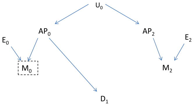
To illustrate our method concretely, we consider health effects of ambient air pollution, although results apply more generally. Thus, exposure is illustrated by air pollutant levels on a specific day (say AP0), measured confounders by meteorologic factors on a specific day (say M0), and the health outcome by asthma emergency department visits on that or a subsequent day (say D1). Figure 2 illustrates these basic relationships. The goal is to assess the effects of exposure (AP0) on disease (D1). Meteorologic factors (M0) affect air pollution levels (AP0) and also affect subsequent disease (D1). For example, M0 might affect disease, perhaps indirectly, by increasing exposure to some other factor (e.g., pollen) that subsequently affects disease. U0 represents an unmeasured factor present on or before day 1, such as an additional unrecognized meteorologic factor, that also affects the air pollutant level (AP0).
Figure 2.

A, the Unmeasured Factor (U0) affects air pollution (AP0) but not disease (D1): B, indicates the same relationships, but U0 also affects Disease.
Figure 2A includes an arrow for each assumed effect: of U0 on AP0; of M0 on AP0; and of M0 on D1. Figure 2B additionally includes an arrow from U0 to D1.
To assess whether control for M0 adequately controls confounding under the assumptions given in Figure 2, we duplicate Figure 2 (A and B) as Figure 3, but make two changes: first, we delete all arrows coming from AP0 to represent blocking the effects of AP0; second, we box in M0 to represent analytic control for it and the blocking of any path through M0. In Figure 3A it is not possible to follow an unblocked path from AP0 back to disease with exposure effects removed, implying no confounding. Without control for M0, an unblocked path from AP0 to D1 is present (through M0) and confounding would be anticipated. On the other hand, with the assumptions incorporated in Figures 2B and 3B, confounding may be present (AP0 and D1 may be associated even if AP0 has no effect on D1) because a backdoor path is present (through U0) even after control for M0.
Figure 3.

As is Figure 2, but arrow from AP0 to disease is removed. A, the unmeasured Factor (U0) affects air pollution (AP0) but not disease (D1): B, indicates the same relationships, but U0 also affects Disease.
These DAGs incorporate our causal assumptions and allow a standard way to evaluate confounding. We now consider an additional variable that, if the causal assumptions are correct, is not a cause of disease but is associated with the exposure. For our motivating example, air pollution levels on a day after the health event has already occurred should satisfy our assumptions. An important presumption is that the health event does not affect subsequent air pollutant concentrations. (This presumption could be invalid if, for example, an increase in health events were noted, thus prompting officials to limit driving or emissions from other sources. Here, we assume this scenario is incorrect.)
We now assume our basic causal structure is correct, with either an unmeasured factor U0 that is not a confounder (as in Figures 2A and 3A) or that is a confounder (Figures 2B and 3B). We also assume that air pollution (AP2) on a day after the health event (D1) is not affected by that event, but like AP0 is affected by the unmeasured factor U0. For example, U0 might be a persistent meteorologic condition that affects air pollution over several days. Figure 4A illustrates that, with our assumptions, AP2 should be (conditionally) independent of disease after control of M0—no unblocked backdoor path exists when U0 is not a confounder. On the other hand, if U0 is a confounder (Fig. 4B) we expect an association of AP2 with disease—an unblocked backdoor path exists even after control of M0. These arguments suggest that we can use a variable, such as air pollutant levels on a day after the health event, as an indicator of unmeasured confounding. Briefly stated, our central assertion is this: if unmeasured confounding is present and our basic causal assumptions reasonably approximate reality, then future air pollution (AP2) can be associated with past disease, whereas in the absence of unmeasured confounding (and given our causal assumptions), AP2 should be independent of past disease. These assertions continue to hold if AP0 is an additional cause of AP2 (i.e., if we add an arrow from AP0 to AP2 in Figures 2 and 3, AP2 is still independent of D0 conditional on AP0 and other measured covariates if confounding is absent, but not necessarily if present). This additional effect is potentially relevant when the indicator used is future exposure.
Figure 4.


A, as in Figure 3A, but also include future value of air pollution (AP2); B, as in Figure 3B, but also include future value of air pollution (AP2).
We show in Appendix 1 that under alternative, more complicated causal assumptions, inclusion of additional, future variables may be useful.
Our arguments have emphasized residual confounding, which is our focus. This might be viewed as a particular type of model misspecification, that due to omission of important factors whose effects mix with and distort the association of interest. Although the primary purpose of the proposed method is decidedly identification of residual confounding, other types of analytic errors could also lead to an association between an “indicator” variable and disease. Hernán and Cole12 note the importance of considering not only confounding but also other types of bias. This is particularly relevant here, as the indicator we propose cannot distinguish between residual confounding, measurement error and misspecification of the dose-response. Any of these biases can lead to an association of the indicator with the outcome; we illustrate this possibility for measurement error in Appendix 2.
Proposed Indicator
We now propose a quantitative indicator for residual confounding based on the presumption that the future ambient air pollutant levels should tend to be associated with disease in the presence of confounding but not associated in its absence. This presumption should be approximated provided the causal relationships discussed above and summarized in Figures 2 and 3 adequately approximate the true relationships.
To use future air pollutant levels as a quantitative indicator, we first fit a model that includes the exposure of interest (air pollutant level prior to disease occurrence, APt) and the relevant covariates, written in general form in Equation (1):
| (1) |
where E(Yt) is the expected value of the count of emergency department visits on day t; APt is a (linear) term for the air pollutant level before or on day t; covariatest is a vector of factors selected for control measured on or before day t; α, β and γ are parameters.
We also fit the same model, but additionally include the indicator (air pollution measured after disease occurrence, APt+1). If residual confounding is absent and the model correctly specified, APt+1 should be unassociated with disease after adjustment for the other variables, and the estimated rate ratio for APt should be little affected by inclusion of APt+1, except perhaps for change in precision. An observed association between APt+1 and disease suggests residual confounding or other potential bias. Although other formulations are possible, here we evaluate the following statistic as an indicator of residual confounding:
| (2) |
where β̈f is the estimated slope for the indicator (e.g. APt+1), when added to the model being assessed for possible misspecification; δ̂f is its estimated standard error. We interpret the statistic I as an approximate z-score, providing a statistical test for confounding.
Simulation Approach
We assess the ability of this approach to detect model misspecification using data from ongoing time-series studies of air pollution and daily emergency department visits. We use simulations so that the true causal relationships will be known, and we use the actual estimated parameters to calculate the “true,” expected daily number of emergency department visits to make the simulations realistic. We base expected counts on daily EDV for asthma over a recent 10-year period in Atlanta (the health event) and use 8-hour maximum ozone levels lagged 1 day as the air pollutant of interest (Table 1). To reduce heterogeneity, we restrict analyses to the warm season (May–October).
Table 1.
Description of Observed Data
| Variable | Mean (SD) | Median/Min/Max |
|---|---|---|
| Daily Asthma ED visits | 50.2 (21.2) | 46/6/144 |
| Daily 8-hour, O31 | 2.28 (0.81) | 2.27/0.28/4.91 |
| Daily Max Temp (C) | 28.4 (4.44) | 29/11/39 |
| Daily Min Temp (F) | 18.2 (4.33) | 19/1/26 |
O3 is measured in units of 25 ppb, approximately equal to its standard deviation.
Analyses use the model given in Equation 1. Covariates include: linear, quadratic and cubic terms for time ( day numbered from 1 to 185 for each 6-month period); linear, quadratic and cubic terms for the moving average of minimum temperature lagged 1–2 days; indicators for temperature on day t (1°C); indicators for day-of-week; indicators for month and year; and product terms between the year and time terms. Emergency department visits counts (Yt) are assumed to be Poisson with mean given by Equation 1. This model is similar, but not identical, to models we have used previously.13
We fit this Poisson model to the observed counts to obtain model-predicted daily counts, which we treat as the truth. For simulations with an assumed non-null air pollution effect, we include APt as a linear term in calculating the expected daily count; for simulations with no assumed air pollution effect, we omit APt+1. We next generate simulated daily counts of emergency department visits with a Poisson distribution and mean given by the model-predicted values. We then analyze each simulated data-set using models that include APt but not APt+1, and models that include both APt and APt+1. Analyses are then conducted that misspecify the analytic model in one of two ways: first, we omit one or more covariates (scenarios 2–6) and, second, we simulate independent (classical) measurement error in the exposure (scenario 7). We calculate the magnitude of confounding in our simulations as the (median) log odds ratio (β̂) estimated with the misspecified model (e.g., a covariate omitted, without the future indicator) minus the true β, where the true β is the coefficient for APt in the model used to generate the simulated data. For scenarios 1A–7A, ozone has no effect in the true model, and for 1B–7B, it does (RR ≈ 1.026 per standard deviation).
To evaluate the ability of the statistic I to detect confounding, we calculate the proportion of simulations in which its absolute value exceeds 1.96, corresponding to rejection of the null (βf=0). We also evaluate its discriminatory ability using the area under the ROC curve (AUC). We calculate the AUC using 500 simulations: we compare (pairwise) I from each generated dataset analyzed with an incorrectly specified model, with I from each generated dataset analyzed with the correctly specified model. The AUC estimate is the proportion of pairs for which I from the incorrectly specified model exceeds I from the correctly specified model, in absolute value.
Results
As shown in Table 2, a small to moderate bias in the log rate ratio was introduced in scenarios 2A – 5A by dropping: day-of-week; time; maximum temperature; and both time and month variables, respectively(column 3 of Table 2). Use of the ozone level one day after the health event discriminated at least somewhat between the correctly and the incorrectly specified model in each scenario. It had weak discriminatory ability in scenario 5A (AUC = 0.60), but the bias in this scenario was relatively small. The ability to discriminate incorrectly from correctly specified models for the other scenarios was better and for scenarios 2A and 4A excellent (AUC ≥ 0.96). The proportion of simulations in which the null (no confounding) is rejected (column 4) tended to increase in parallel with the AUC. Addition of the future meteorologic factor as another control variable tended to weaken the ability of the indicator to distinguish an incorrectly from a correctly specified model (rightmost column, Table 2).
Table 2.
Simulation Results, True Model stipulates No Effect of Exposure (Ozone, lagged 1 day) on Asthma ED visits
| Scenario | Type of Analytic Error (Misspecification) | Bias1: Median β̂-True β (SE (β̂)) | Proportion of Simulations in which Null (Ho: βf =0) is Rejected2 | AUC 3 (Future AP only) | AUC Future AP +Future Meteorological |
|---|---|---|---|---|---|
| 1A | None | 0.0006 (0.0056) | 0.052 | - | |
| 2A | Omit day of week indicators | 0.0070 (0.0071) | 0.773 | 0.96 | 0.95 |
| 3A | Omit continuous time variables (t, t2,t3) | −0.0077 (0.0071) | 0.441 | 0.86 | 0.46 |
| 4A | Omit continuous time variables and Month indicators | −0.0439 (0.0094) | 1.00 | 0.98 | 0.49 |
| 5A | Omit Maximum Temperature Indicators | 0.0112 (0.0049) | 0.136 | 0.60 | 0.51 |
| 6A | Omit Minimum and Max Temperature Variables | 0.0127 (0.0050) | 0.244 | 0.70 | 0.50 |
| 7A | Add Measurement Error | 0.0001 (0.0021) | 0.062 | 0.51 | 0.51 |
Median bias: median β̂- true β, in models without APt+1.
Proportion of simulations in which the null (βf = 0) is rejected.
The AUC is 0.5 in the absence of discriminatory ability and 1.0 for perfect discriminatory ability.
When the exposure had an effect in the “true” model (RR ≈ 1.026), results were generally similar (Table 3): the statistic I had some ability to distinguish misspecified from correctly specified models, but again this differed by scenario. In scenario 5B, omission of maximum Temperature led to little bias and discriminatory ability was weak (AUC = 0.51), likely due in part to the weak confounding.
Table 3.
Simulation Results, True Model Stipulates an Effect of Exposure (Ozone, lagged 1 day) on Asthma ED visits
| Scenario | Type of Analytic Error (Misspecification) | Bias1: Median β̂- True β̂ (SE (β̂)) | Proportion of Simulations in which Null (Ho: βf =0) is Rejected2 | AUC3 (Future AP only) | AUC Future AP + Future Meteorological Factor |
|---|---|---|---|---|---|
| 1B | None | 0.0006 (0.0056) | 0.050 | - | - |
| 2B | Omit day of week indicators | 0.0061 (0.0071) | 0.768 | 0.96 | 0.96 |
| 3B | Omit continuous time variables (t, t2,t3) | −0.0092 (0.0071) | 0.493 | 0.88 | 0.55 |
| 4B | Omit continuous time variables and Month indicators | −0.0109 (0.0073) | 1.00 | 1.00 | 0.51 |
| 5B | Omit Max Temperature Variables | 0.0047 (0.0050) | 0.060 | 0.51 | 0.91 |
| 6B | Omit Minimum and Max Temperature Variables | 0.0055 (0.0050) | 0.098 | 0.56 | 0.50 |
| 7B | Add Measurement Error | −0.0221 (0.0021) | 0.070 | 0.53 | 0.50 |
Median bias: median β̂- true β, in models without APt+1.
Proportion of simulations in which the null (βf = 0) is rejected.
The AUC is 0.5 in the absence of discriminatory ability and 1.0 for perfect discriminatory ability.
We also evaluated a formulation of the indicator based on the change in the coefficient (β) for the exposure of interest (APt) in models with and without APt+1 divided by its standard error in the model without APt+1,(β̂1 − β̂2)/δ̂1. The discriminatory ability of this alternative indicator was similar to that for I (data not shown).
We chose ozone and emergency department visits related to asthma in order to illustrate and evaluate performance of the method because we previously found13 a strong link between ozone and asthma. For completeness, we also simulated results for visits related to cardiovascular disease and lag 0 (same day) carbon monoxide (CO). The ability of the indicator to detect confounding for this disease and exposure was less, sometimes essentially absent (data not shown). This likely occurred for three reasons: first, the degree of confounding for each scenario was substantially less than the corresponding scenario for asthma-ozone; second, the correlation of the indicator with the exposure was weaker for CO than for ozone (0.33 vs. 0.51, respectively); and finally, the correlation of the future indicator (future CO) with the omitted factors also tended to be substantially less (e.g., for Maximum Temperature: −0.04 vs. 0.49 with CO and ozone, respectively).
Discussion
The proposed method can detect important, residual confounding—its primary purpose. For some types and degrees of residual confounding, the discriminatory ability was excellent, but it was weak for others. However, situations in which discriminatory ability was weakest tended to be those with less confounding, at least for the examples considered. The indicator may be most useful for comparing competing models—for choosing between models that seem reasonable based on a priori considerations of causal relationships. The model with the weakest indication of misspecification might be preferred, although sensitivity analyses would nevertheless remain useful. Models with stronger indications of misspecification might be less preferred.
As noted previously, the proposed indicator cannot distinguish among confounding, measurement error and misspecification of the dose-response, all potentially important sources of bias. However, if interest is in characterizing ambient air pollutant levels, measurement error is arguably relatively lower by definition: even if ambient pollutant levels imperfectly measure actual exposures, they can be feasibly measured with better accuracy than true exposures (e.g., for all residents of a city), and then regulated and changed. Thus, ambient levels can be conceptually valid exposures and appropriate objects of study.14 Furthermore, if measurement error estimates are available, then correction for measurement error is possible,15 although utility of the many applicable methods may be limited by the information available.
The proposed method is firmly rooted in the concepts of causality and confounding. In particular, we have assumed that the causal patterns summarized in the DAGs appropriately reflect the important relationships; if not, the approach may fail. The described application to time series also hinges on the requirement that a cause must precede its effect so that an association with a factor that occurs after the outcome cannot be its cause. If we also assume that the disease does not affect the indicator, then associations between such a factor and the outcome must reflect an association other than a direct causal effect of the indicator on disease (or the reverse). Likely explanations are residual confounding or perhaps measurement error or misspecification of form of the concentration-response. We reiterate that the primary purpose of the proposed approach is not identification of measurement error or misspecification of form because other, more direct methods are available to identify these problems.6,16 Our method provides an indicator for detecting the more elusive residual confounding, possibly due to unmeasured or unrecognized factors.
We have justified and evaluated the proposed method in the context of time-series studies of the effects of air pollution (ozone and CO) on emergency department visits (asthma and cardiovascular disease), but the method applies to other types of studies as well. If a factor is available that does not cause the outcome of interest, but that is associated with the exposure and any omitted confounder, one can evaluate applicability of the method by using DAGs. As general examples, the method may be applicable in certain other types of time-series studies and in genetic studies. In genetic studies, the indicator might be the genotype of a spouse or offspring of the subject whose disease risk is assessed in the study. If there is no confounding, say by population stratification, then neither the spouse’s nor the child’s genotype should be associated with the presence of (many types of) disease in the subject, conditional on that subject’s genotype. The presumption is that a spouse’s or child’s genotype does not affect the subject’s disease; conditional on the subject’s genotype, that of the spouse or child is irrelevant. However, if an unmeasured cultural factor is associated with the genotype under investigation and is also a risk factor, leading to residual confounding, then that factor should be associated with the spouse’s genotype—and should manifest as an association between the genotype of the child or spouse and the subject’s disease, even conditional on the subject’s genotype.
In review, Dr. Robins pointed out that our proposed approach can be justified using results of the G-computation algorithm.17 In particular, we can consider the Disease (Dt) as a treatment. In the absence of confounding, the G-formula for the effect of Dt on APt+1, conditional on covariates through time t, is the regression of APt+1 on Dt conditional on measured covariates. An association of Dt with APt+1 suggests violation of the no confounding assumptions whereas no association is consistent with that assumption. This approach provides another way to justify our conclusions. We note that we are not the first to use this future indicator. For example, some of us13 as well as others18 used it previously but without providing the theoretical justification (apart from a presentation and abstract19). After we submitted this manuscript, Lipsitch et al20 described a “negative control exposure” for detecting confounding. Their concept of a negative control exposure (it “should ideally have the same incoming arrows as [the exposure]”20) overlaps with ours of an indicator (“when the model is correctly specified [it] must be conditionally independent of the outcome given exposure and any other modeled covariate[,]… associated with the exposure of interest and, like that exposure, with the (possibly unmeasured) confounders”). But the concepts also differ, perhaps because Lipsitch and colleagues did not consider future exposure as a possible indicator. Our indicator is likely not an ideal negative control exposure, particularly if based on future exposures or the child’s genotype as in the examples above. We now explicitly note above that causes of the indicator can validly include exposure itself, implying that the restriction (negative control exposure and exposure itself have the same causes) can be relaxed. Thus, the two concepts are similar, yet nevertheless have important differences.
Although our method generalizes to other kinds of studies and situations, our simulation results may not. Other pollutants, outcomes and models would have different discriminatory ability; simulations specific to those situations should yield more directly applicable estimates of discriminatory ability. We could calculate the AUC to evaluate the predictive ability of the indicator because we specified the true model for the simulations; in analyses of actual data, the AUC would not be available because the true model is unknown. Nevertheless, the indicator can be calculated to assess and test model misspecification. Simulations could also be done to evaluate the indicator under conditions similar to those arising in actual analyses.
The method can be modified by including future values of factors other than those for the exposure, such as meteorologic factors, either as a control or as an additional indicator variable. In our simulations, however, we assessed whether additional discriminatory ability accrued by controlling for future meteorologic variables while still using future air pollutant levels as the indicator. These simulations suggested the discriminatory ability of the indicator was weakened by controlling for future meteorologic variables, but this result may be sensitive to the situation considered. On the other hand, we did not evaluate use of the future meteorologic variable itself as the indicator. The indicator used here (I = β̂f)/δ̂f ) should have an approximate Gaussian distribution for large studies. However, this distribution might not directly apply for some other indicators, such as the change in the estimated slope for the exposure of interest induced by including the indicator. Furthermore, the approach hinges on the assumed causal relationships, the validity of which is not readily captured by a P-value. Thus, we encourage full consideration of all causal relationships, available a priori information, the magnitude of the indicator I and sensitivity analyses in addition to the z-score calculated from I when assessing confounding. More evaluation remains for different outcomes, pollutants and indicators and for applications in other fields, such as genetics.
In the situations considered, the method tended to provide the strongest indication of misspecification when it was due to unmeasured confounding; discriminatory ability was weak for detecting measurement error and even weaker for misspecification of the dose-response (data not shown). In a few scenarios with a relatively large rate ratio (e.g., 1.15) and no lag for the exposure of interest, such that the correlation between the indicator and exposure was strong, the indicator had discriminatory ability for classical exposure measurement error (AUC as high as 0.9; data not shown). However, we do not view the greater discriminatory ability for unmeasured confounding as a weakness, because this situation is consistent with the primary purpose of the proposed approach. Rather, we note that, if the indicator suggests a problem, we must also consider these other sources of analytic error, because the indicator does not distinguish among them.
In summary, we have proposed and evaluated an approach for identifying residual confounding. It is justified by appeal to causal models, requiring availability of a factor that cannot plausibly cause the outcome, but that should be associated with the exposure of interest and, like it, with potential confounders as described in the causal diagrams. Simulations suggest that it can have discriminatory ability for the identification of residual confounding due to unmeasured risk factors, but the strength of this ability will vary according to the situation. It provides an additional tool for assessment of residual confounding—one that uses a priori knowledge in a novel way and that builds on the causal nature of confounding.
Acknowledgments
Funding: This work was supported by the following grants: EPA STAR RD83479901 and RD833626, NIEHS R01ES11294 and EPRI EP-P277231/C13172. The views expressed in this document are solely those of the authors and do not necessarily reflect the views of the funding agencies, and mention of any products or commercial services does not constitute endorsement.
Appendix 1 Other Causal Relationships
We now consider a slightly more complicated situation in which a second, unmeasured factor (say, Uo*) affects both disease and future meteorological factors, as shown in Figure 5. In this case, no confounding path involving Air Pollution (AP0) is present, as there is no unblocked backdoor path from AP0 to disease (D1) although a confounding path from M0 to D1 is present.
Figure 5.

The Unmeasured Factor (U0) affects air pollution (AP0) but not disease (D1), and the unmeasured factor (U0*) affects meteorology (M0), future meteorology (M2) and disease.
If we use the association of emergency department visits with AP2 as an indicator of unmeasured confounding, we would expect to find an association by the path from AP2 to M2 to U0* to D1 (dotted, curved line in Figure 6). However, if we also include the future meteorologic variable (M2) as a control variable, then this backdoor path is blocked once we control for M2, and we would expect to find no unblocked path and therefore no association between AP2 and disease, D1 (Figure 7). Thus, the “test” should correctly not indicate residual confounding involving AP0, provided we control for M2. In summary, assuming the causal situation in Figure 7 in which there is no confounding, we expect no association between the indicator (AP2) and disease, provided we also control for the future meteorologic variable (M2), but would expect an association even without confounding by Uo if we did not control for M2. On the other hand, if there is confounding as represented by an effect of Uo on D1, we would expect an association between the indicator (AP2) and disease even if we control for M2 (Figure 8). Control for the additional meteorologic variable (M2) can improve the ability to correctly distinguish absence of a confounding path involving AP0 from its presence.
Figure 6.

Indicates the association between future air pollution (AP2) and disease (D1), due to presence of the unmeasured factor U0*. The (other) unmeasured Factor (U0) affects air pollution (AP0) but not disease (D1); U0* affects meteorology (M0), future meteorology (M2) and disease.
Figure 7.

Control for the future meteorologic factor (M2) eliminates the association between future air pollution (AP2) and disease.
Figure 8.

As in Figure 7, U0 also affects disease (D1), so confounding is suspect. Control for the future meterologic factor (M2) no longer eliminates the association between future air pollution (AP2) and disease.
Appendix 2 Measurement Error
We now consider the impact on the indicator of measurement error, that is use of an exposure that is measured with error, another possible source of bias. In the presence of measurement error, exposure measured after disease has already occurred could be correlated with the underlying (but mis-measured) true exposure on previous days, even conditional on the measured exposure for previous days, and be associated with disease. This possibility is illustrated in Figure 9, which shows a backdoor path from M2, the measured value of future air pollution, to D1 even after control for the measured value (M0) of the air pollution of interest (AP0). Yet another type of misspecification would involve inclusion of the wrong form of an exposure or covariates (e.g., the exposure is included in the model as a linear term but the correct dose-response is nonlinear). Again, exposure measured after disease has already occurred could be correlated with the correct exposure term and be associated with disease. Thus, we expect that the indicator may be associated with disease, not only if an important confounder is omitted, but also if the model is misspecified or measurement errors of important causal factors are correlated with the indicator.
Figure 9.
Measurement error (E0 and E1) affects the measured air pollution levels (M0 and M1, respectively). The true air pollution level (AP0), affects disease, but the future level (AP2) does not have this effect.
References
- 1.Hastie T, Tibshirani R, Friedman J. The Elements of Statistical Learning. New York: Springer-Verlag; 2001. [Google Scholar]
- 2.Peng RD, Dominici F, Louis TA. Model choice in time series studies of air pollution and mortality. Roy Stat Soc A. 2006;169:179–203. [Google Scholar]
- 3.Greenland S, Pearl J, Robins J. Causal Diagrams for Epidemiologic Research. Epidemiol. 1999;10:37–48. [PubMed] [Google Scholar]
- 4.Robins J. Data, design, and background knowledge in etiologic inference. Epidemiology. 2001;12(3):313–20. doi: 10.1097/00001648-200105000-00011. [DOI] [PubMed] [Google Scholar]
- 5.Hernan MA, Hernandez-Diaz S, Werler MM, Mitchell AA. Causal knowledge as a prerequisite for confounding evaluation: an application to birth defects epidemiology. Am J Epidemiol. 2002;155(2):176–184. doi: 10.1093/aje/155.2.176. [DOI] [PubMed] [Google Scholar]
- 6.Rothman KJ, Greenland S, Lash TL. Modern Epidemiology. 3. Philadelphia: Lippincott Williams & Wilkins; 2008. [Google Scholar]
- 7.Granger CWJ. Testing for causality: a personal viewpoint. J Economic Dynam Control. 1980;2:329–352. [Google Scholar]
- 8.Hendry DF. The Nobel Memorial Prize for Clive WJ. Granger Scand J Econom. 2004;106:187–213. [Google Scholar]
- 9.Greenland S, Robins JM. Identifiability, exchangeability, and epidemiological confounding. Int J Epidemiol. 1986;15(3):413–9. doi: 10.1093/ije/15.3.413. [DOI] [PubMed] [Google Scholar]
- 10.Robins JM, Greenland S, Hu FC. Estimation of the causal role of a time-varying exposoure on the marginal mean of a repeated binary outcome. J Am Stat Assoc. 1999;94:687–700. [Google Scholar]
- 11.Robins J. General methodologic considerations. J Econometrics. 2003;112:89–106. [Google Scholar]
- 12.Hernan MA, Cole SR. Invited Commentary: Causal Diagrams and Measurement Bias. Am J Epidemiol. 2009;170(8):959–962. doi: 10.1093/aje/kwp293. [DOI] [PMC free article] [PubMed] [Google Scholar]
- 13.Peel JL, Tolbert PE, Klein M, Metzger KB, Flanders WD, Todd K, Mulholland JA, Ryan PB, Frumkin H. Ambient air pollution and respiratory emergency department visits. Epidemiol. 2005;16(2):164–174. doi: 10.1097/01.ede.0000152905.42113.db. [DOI] [PubMed] [Google Scholar]
- 14.Zeger SL, Thomas D, Dominici F, Samet JM, Schwartz J, Dockery D, Cohen A. Exposure measurement effort in tme-series studies of air pollution: concepts and consequences. Environ Health Perspect. 2000;108:419–426. doi: 10.1289/ehp.00108419. [DOI] [PMC free article] [PubMed] [Google Scholar]
- 15.Armstrong BG. Effect of measurement error on epidemiologic studies of environmental and occupational exposures. Occupat Environ Med. 1998;55:651–656. doi: 10.1136/oem.55.10.651. [DOI] [PMC free article] [PubMed] [Google Scholar]
- 16.Neter JWW, Kutner MH. Applied Regression Models. Boston: Irwin; 1989. [Google Scholar]
- 17.Robins J. A new approach to causal inference in mortality studies with sustained exposure periods-application to control of the health worker survivor effect. Mathematical Modeling. 1986;7:1393–1515. [Google Scholar]
- 18.Dominici F, Peng RD, Bell ML, Pham L, McDermott A, Zeger SL, Samet JM. Fine particulate air pollution and hospital admission for cardiovascular and respiratory diseases. JAMA. 2006;295:1127–1134. doi: 10.1001/jama.295.10.1127. [DOI] [PMC free article] [PubMed] [Google Scholar]
- 19.Flanders WD, Klein M, Strickland M, Darrow L, Sarnat S, Sarnat J, Waller L, Tolbert PE. A method of identifying residual confounding and other violations of model assumptions. Epidemiol. 2009:s44–s45. [Google Scholar]
- 20.Lipsitch M, Tchetgen E, Cohen T. Negative Controls: A Tool for Detecting Confounding and Bias in Observational Studies. Epidemiology. 2010;21(3):383–388. doi: 10.1097/EDE.0b013e3181d61eeb. [DOI] [PMC free article] [PubMed] [Google Scholar]