Analysis of Longitudinal Shape Variability via Subject Specific Growth Modeling

Abstract

Statistical analysis of longitudinal imaging data is crucial for understanding normal anatomical development as well as disease progression. This fundamental task is challenging due to the difficulty in modeling longitudinal changes, such as growth, and comparing changes across different populations. We propose a new approach for analyzing shape variability over time, and for quantifying spatiotemporal population differences. Our approach estimates 4D anatomical growth models for a reference population (an average model) and for individuals in different groups. We define a reference 4D space for our analysis as the average population model and measure shape variability through diffeomorphisms that map the reference to the individuals. Conducting our analysis on this 4D space enables straightforward statistical analysis of deformations as they are parameterized by momenta vectors that are located at homologous locations in space and time. We evaluate our method on a synthetic shape database and clinical data from a study that seeks to quantify brain growth differences in infants at risk for autism.

1 Introduction

Quantification of anatomical variability within a population and between populations are fundamental tasks in medical imaging studies. In many clinical applications, it is particularly crucial to quantify anatomical variability over time in order to determine disease progression and to isolate clinically important differences in both space and time. Such studies are designed around longitudinal imaging, where we acquire repeated measurements over time of the same subject, which yields rich data for analysis. Statistical analysis of longitudinal anatomical data is a problem with significant challenges due to the difficulty in modeling anatomical changes, such as growth, and comparing changes across different populations.

Many methods have been proposed for the statistical analysis of cross-sectional time-series data, which do not contain repeated measurements of the same subject. Methods include the extension of kernel regression to Riemannian manifolds [1] or piecewise geodesic regression for image time-series [6]. Others have proposed higher order regression models, such as geodesic regression [9,4], regression based on stochastic perturbations of geodesic paths [11], or regression based on twice differential flows of deformation [3].

A method for the analysis of longitudinal anatomy was proposed recently in [2], where a longitudinal atlas is constructed by considering each individual subject as a spatiotemporal deformation of a mean scenario of growth. A single spatial deformation maps the geometry of the atlas onto the observed individual geometry, while a 1D time warp accounts for pacing differences between the atlas and subjects. In this framework, statistics are naturally performed on the initial momenta that parameterize the morphological deformation to each subject. However, this single deformation best explains how the entire evolution of the mean scenario maps to each individual. The analysis of shape variability at an arbitrary time point has not been explored.

Methods for constructing a longitudinal atlas for DTI [5] and images [7] have been introduced by combining subject specific growth modeling with cross-sectional atlas construction. As a first step, a continuous evolution is estimated for each subject using the standard piecewise geodesic regression model. The continuous evolution for all subjects is then used to compute a cross sectional atlas. Lastly, subjects are registered to the atlas space by the same regression technique used to establish individual trajectories. Though subject specific growth trajectories are incorporated, the cross-sectional atlas building step is likely to smooth intra-subject variability, as only the images themselves are used for atlas construction; the trajectories are ignored.

In this paper, we propose a new approach for analyzing statistical variability of shapes over time, in the spirit of [5,7], which is based on combining cross-sectional atlas construction with subject specific growth modeling. The growth model used for shape regression naturally handles multiple shapes at each time point and does not require point correspondence between subjects, making the proposed framework both convenient and applicable to a wide range of clinical problems. We demonstrate the application of our modeling and analysis framework to a synthetic database of longitudinal shapes as well as a study that seeks to quantify growth differences in subjects at risk for autism.

2 Methods

The proposed framework consists of three steps, summarized in Fig. 1. First, a cross-sectional atlas is estimated by shape regression, which can be thought of as normative, reference evolution. Second, subject specific growth trajectories are estimated independently for each individual, accounting for intra-subject variability. Third, a homologous space for statistical analysis is obtained by warping the atlas to each individual at any time point of interest. The first two steps require the estimation of a growth model, the specifics of which are discussed in the next section.

Fig. 1.

Flowchart depicting the proposed method.

2.1 Growth Model

The goal is to infer a continuous evolution of shape from a discrete set of shapes S_ti observed at time t_i. Here we use the acceleration controlled growth model of [3], where shape evolution is modeled as a continuous flow of deformation. A baseline shape S₀, assumed to be observed at time t₀, is continuously deformed over time to match the target shapes. The estimation is posed as a variational problem balancing fidelity to data with regularity, described by the generic regression criterion

$$E=\sum _{t_i}d{({\phi }_{t_i}(S_0),S_{t_i})}^2+\gamma \text{Reg}({\phi }_t)$$ (1)

where φ_t is the time-varying deformation we wish to estimate, d is a measure of shape similarity, Reg is a regularity constraint on the flow of deformation, and γ is the trade-off parameter. The time-varying deformation φ_t is determined by integration of the 2nd-order ODE φ̈_t(x_i(t)) = a(x_i(t), t), where a is a time-varying acceleration field, and x_i(t) are the location of shape points over time.

The parameterization by acceleration guarantees that the estimated evolution is temporally smooth. Furthermore, the acceleration controlled growth model is generic, with no constraint that the flow of deformation must follow a geodesic path, or close to a geodesic path.

For measuring shape similarity, we use the metric on currents [10]. This way, shapes are modeled as distributions, alleviating the need for explicit point correspondence between shapes. Regularity is enforced via a Hilbert space norm on acceleration, ${\left|\right|\mathit{a}\left|\right|}_V^2$ defined by the interpolating kernel.

The choice of metric and regularization leads to two intuitive parameters to control the estimation. First, λ_V controls the rigidity of the deformation. It is the scale that points in space move in a correlated manner. Small values of λ_V lead to highly non-linear deformations, while large values result in mostly rigid transformations. The second parameter, λ_W is the scale at which geometric shape differences are considered noise. Shape variations smaller than λ_W are ignored in computing shape similarity.

2.2 Matching Atlas to Individuals

We extract shape features, which are diffeomorphisms that map the reference atlas to each subject at a specific time point. This is accomplished by warping the atlas to each subject at the time point of interest using the registration framework of [10]. Due to regression, we can construct a shape from the atlas and from any individual at any time of interest. The warping from atlas space to each individual establishes homologous points between every subject. The flow of diffeomorphisms that match the atlas shape A(t) to subject shape S^s(t) at time t is found as the minimizer of

$$F(t)=d{({\phi }_t^s(A(t)),S^s(t))}^2+\gamma \text{Reg}({\phi }_t^s)$$ (2)

where d is the norm on currents, and regularity enforces smoothness on the time-varying velocity field, which is used to build the diffeomorphism.

2.3 Statistical Analysis

The flow of diffeomorphisms that warp the template shape to each individual subject shape are geodesic [8]. As a result, the initial momenta completely determine the entire deformation. Since the atlas is warped to each subject, every diffeomorphism ${\phi }_t^s$ starts from the same reference space. We can leverage this common vector space to compute intrinsic statistics. For example, a mean can be computed by simply taking the arithmetic mean of a collection of momenta fields. The mean momenta can then be applied to a shape via geodesic shooting.

3 Experiments

Synthetic Data

We first evaluate our framework with a database of synthetic longitudinal shape data. In this simple database, normative growth is modeled by a sphere which grows isotropically over time. We further consider two groups, A and B, with different patterns of growth. Group A starts as a small sphere, develops a protuberance in the negative x direction, and eventually evolves into a large sphere. Group B also starts from a small sphere, but develops a protuberance in the positive x direction, before evolving into a large sphere. Subjects from both groups contain 5 time points corresponding to 6, 10, 12, 18, and 24 months. We construct 12 subjects in each group by randomizing the amount of protuberance and also the amount of global scaling. A typical subject from group A and group B as well as the normative reference growth are summarized in Fig 2.

Fig. 2.

The synthetic shape database with observations at 6, 10, 12, 18, and 24 months. Top: Typical shape observations for a subject from group A. Middle: The normative growth scenario. Bottom: Typical shape observations for a subject from group B.

The normative reference atlas is estimated from a collection of spheres of increasing radius using parameter values λ_V = 0.5 mm, λ_W = 0.5 mm, and γ_R = 0.0001. We further estimate individual growth models for all 24 subjects using the same parameter values as for normative growth. The continuous evolution for both the normative group and all individuals provides temporal correspondence, as we can now generate shapes at any instant in time. The atlas shapes at time points 7, 9, 12, 18, and 24 months are then warped to each individual via a diffeomorphic mapping.

First, we perform PCA on the momenta that warp the normative atlas to each individual in group A. The first major mode of variation is summarized in Fig 3 for several time points. This mode explains the variability in group A with respect to the reference shapes. The bulge on the left side of the shape is clearly identified along with variability in scale. A PCA on group B produces similar results, however it captures the bulge on the right side of the shape.

Fig. 3.

The first major mode of deformation from PCA (mean plus one standard deviation) at selected time points for group A. Color indicates the displacement from the mean shape. The variability in the protuberance is clearly captured.

We also conduct hypothesis testing to determine if there are significant differences between group A and B. For each shape point, an independent t-test is performed on the magnitude of initial momenta which parameterize the mapping from reference atlas to individuals. We are testing if the distribution of momenta magnitude at each shape point is different between each group. Fig 4 shows the Bonferroni corrected p-values shown on the reference atlas at selected time points. We observe significance on the left and right side of the shapes at 9, 12, and 16 months, corresponding to the bulge growing in opposite directions in group A and B. It is also important to note that we observe no significant differences at 20 months, where the shapes of each group are nearly identical.

Fig. 4.

Significant differences in magnitude of momenta between group A and B at several time points, with p-values displayed on the surface of the reference atlas.

Clinical Data

We also evaluate our method using a longitudinal database from an Autism Center of Excellence, part of the Infant Brain Imaging Study (IBIS). The study consists of high-risk infants as well as controls, scanned at approximately 6, 12, and 24 months. At 24 months, symptoms of autism spectrum disorder (ASD) were measured using the Autism Diagnostic Observation Schedule (ADOS). A positive ADOS score indicates the child has a high probability of later being diagnosed with autism. Finally, we have three groups: 15 high-risk subjects with positive ADOS (HR+), 40 high-risk subjects with negative ADOS (HR−), and 14 low-risk subjects with negative ADOS (LR−).

We perform a hierarchical, multi-scale rigid alignment to establish a common reference frame that preserves the relationship between anatomical structures in space and time. First, left/right hemisphere and cerebellum are segmented from rigidly aligned images. Next, for each individual, shape complexes are aligned across time. Finally, individual shapes are aligned across time for each subject.

First, we estimate a cross-sectional atlas of normative growth using all the data from the LR− group with parameters values λ_V = 30 mm, λ_W = 10 mm for each hemisphere and λ_W = 8 mm for the cerebellum, and λ_R = 0.01. Individual trajectories are estimated independently for each subject using the same parameter values. Finally, we investigate the shape variability at 7, 9, 12, 18, and 24 months by registering the atlas to every subject at the time points of interest, resulting in diffeomorphic mappings parameterized by initial momenta.

We investigate the shape variability in the HR+ and HR− groups by performing PCA on the initial momenta for each group. Recall that PCA is conducted using the momenta vectors that parameterize the mapping from atlas to subject at each selected time point. Therefore, the major modes of variability describe how each group varies from the normative growth scenario, shown in Fig. 5 for several time points of interest. There appears to be a difference in how each group deviates from the normative growth scenario, particularly in the cerebellum. This could be an interesting avenue to pursue for future research.

Fig. 5.

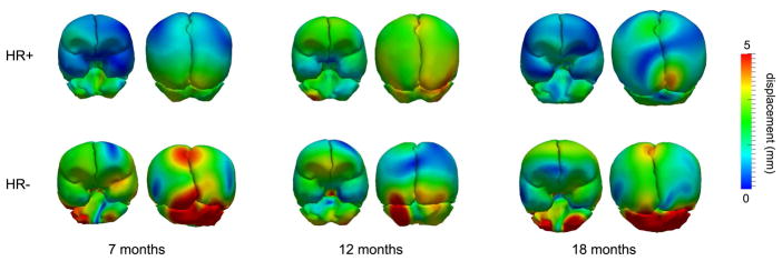
The first mode from PCA (mean plus one standard deviation) at selected time points for the autism database. Color indicates displacement from the mean shape.

Hypothesis testing is conducted on the magnitude of initial momenta between groups. For each shape point, we perform a t-test on the distribution of momenta magnitude between each population. After correcting the p-value for multiple comparisons, using Bonferroni correction, we find no significant locations on the surfaces of the left/right hemisphere or cerebellum. This may be due to relatively small sample size. However, it may be the case that smaller scale anatomical surfaces, such as subcortical structures might lead to group discrimination due to hypothesized differences in brain growth.

It is important to stress that these results are intended to illustrate a potential application of our methodology. The results here are too preliminary to draw meaningful conclusions with respect to autism, due to the small sample size and the need to incorporate biostatistical modeling, that combines patient variables with our computational analysis.

4 Conclusions

We propose a new approach for analyzing shape variability over time, and for quantifying spatiotemporal population differences. Our approach estimates anatomical growth models over time for a reference population (an average model) and for individuals in different groups. We define a reference 4D space for our analysis as the average population model and measure shape variability through diffeomorphisms that map the average to the individuals. Conducting our analysis on this 4D space enables straightforward statistical analysis of deformations as they are parameterized by momenta vectors that are located at homologous locations in space and time.

We validated our approach on synthetic data, demonstrating that we can detect significant differences between two groups with different growth trajectories. Experiments on anatomical data from an autism study show that there is no significant difference in the brain development of high risk children with positive and negative ADOS scores, as compared to the development of controls. In the future, we plan to extend the framework by modeling the intra-subject variability in the reference population.

References

- 1.Davis B, Fletcher P, Bullitt E, Joshi S. ICCV. IEEE; 2007. Population shape regression from random design data; pp. 1–7. [Google Scholar]
- 2.Durrleman S, Pennec X, Trouvé A, Gerig G, Ayache N. Spatiotemporal atlas estimation for developmental delay detection in longitudinal datasets. In: Yang GZ, Hawkes D, Rueckert D, Noble A, Taylor C, editors. MICCAI. LNCS. Vol. 5761. Springer; 2009. pp. 297–304. [DOI] [PMC free article] [PubMed] [Google Scholar]
- 3.Fishbaugh J, Durrleman S, Gerig G. Estimation of smooth growth trajectories with controlled acceleration from time series shape data. In: Fichtinger G, Peters T, editors. MICCAI. LNCS. Vol. 6892. Springer; 2011. pp. 401–408. [DOI] [PMC free article] [PubMed] [Google Scholar]
- 4.Fletcher P. Geodesic Regression on Riemannian Manifolds. In: Pennec X, Joshi S, Nielsen M, editors. MICCAI Workshop on Mathematical Foundations of Computational Anatomy. 2011. pp. 75–86. [Google Scholar]
- 5.Hart G, Shi Y, Zhu H, Sanchez M, Styner M, Niethammer M. DTI longitudinal atlas construction as an average of growth models. In: Gerig G, Fletcher P, Pennec X, editors. MICCAI Workshop on Spatiotemporal Image Analysis for Longitudinal and Time-Series Image Data. 2010. [Google Scholar]
- 6.Khan A, Beg M. ISBI. IEEE; 2008. Representation of time-varying shapes in the large deformation diffeomorphic framework; pp. 1521–1524. [Google Scholar]
- 7.Liao S, Jia H, Wu G, Shen D. A novel longitudinal atlas construction framework by groupwise registration of subject image sequences. NeuroImage. 2012;59(2):1275–1289. doi: 10.1016/j.neuroimage.2011.07.095. [DOI] [PMC free article] [PubMed] [Google Scholar]
- 8.Miller MI, Trouvé A, Younes L. On the metrics and Euler-Lagrange equations of Computational Anatomy. Annual Review of Biomedical Engineering. 2002;4:375–405. doi: 10.1146/annurev.bioeng.4.092101.125733. [DOI] [PubMed] [Google Scholar]
- 9.Niethammer M, Huang Y, Vialard FX. Geodesic regression for image time-series. In: Fichtinger G, Peters T, editors. MICCAI. LNCS. Vol. 6982. Springer; 2011. pp. 655–662. [DOI] [PMC free article] [PubMed] [Google Scholar]
- 10.Vaillant M, Glaunès J. IPMI. LNCS. Vol. 3565. Springer; 2005. Surface matching via currents; pp. 381–392. [DOI] [PubMed] [Google Scholar]
- 11.Vialard F, Trouvé A. Shape splines and stochastic shape evolutions: A second-order point of view. Quarterly of Applied Mathematics. 2012;70:219–251. [Google Scholar]