The multivariate beta process and an extension of the Polya tree model

Summary

We introduce a novel stochastic process that we term the multivariate beta process. The process is defined for modelling-dependent random probabilities and has beta marginal distributions. We use this process to define a probability model for a family of unknown distributions indexed by covariates. The marginal model for each distribution is a Polya tree prior. An important feature of the proposed prior is the easy centring of the nonparametric model around any parametric regression model. We use the model to implement nonparametric inference for survival distributions. The nonparametric model that we introduce can be adopted to extend the support of prior distributions for parametric regression models.

1. Introduction

We introduce a stochastic process that we call the multivariate beta process; this is not related to the process introduced in Hjort (1990). The multivariate beta process {Y_x}_x∈X is defined on a Euclidean space X ⊂ 𝕉^k, for every x in X, the random variable Y_x has a beta distribution and, for every pair of points (x₁, x₂) in X, the random variables Y_x1 and Y_x2 are positively dependent. Moreover, the degree of dependence becomes stronger as x₁ approches x₂. In the first part of this article, the multivariate beta process is studied and a relation with the Dirichlet process (Ferguson, 1974) is illustrated. In the second part, a Bayesian model for a family 𝒫 = {𝒫_x; x ∈ X} of dependent random probability measures 𝒫_x indexed by covariates x is defined by using the multivariate beta process. The model is an extension of the Polya tree model (Lavine, 1992).

Many important applications naturally lead to statistical inference based on dependent random distributions. Typical examples are MacEachern (1999), De Iorio et. al. (2004) and Dunson & Park (2008). We use the proposed model to implement a nonparametric extension of a parametric proportional hazards model.

The stochastic process 𝒫 is indexed by the points of the set {X × 𝒝}, where X is the covariate space and 𝒝 is the usual Borel σ-field of the real line. It is assumed that X ⊂ 𝕉^k, for a given positive integer k: covariates can be continuous or discrete. We summarize a few salient properties of the model. For any x ∈ X, the marginal process {𝒫_x (B)}_B∈𝒝 is a random probability measure with a Polya tree distribution. The process can a priori be centred around a given regression model {F_x}_x∈X. The model {F_x}_x∈X can include unknown hyperparameters θ. For example, in an application to survival data, we use a Weibull model with unknown regression parameters θ for prior centring. Another relevant property of the model is that for every measurable subset B ∈ 𝒝, point x ∈ X and sequence {x_i ∈ X}_i⩾1 such that the Euclidean distances {‖ x_i − x ‖}_i⩾1 vanish, the random sequence {𝒫_xi (B)}_i⩾1 converges in probability to 𝒫_x (B). We also illustrate that, for every finite subset of the covariate space {x₁, …, x_m}, the law of the random probability measures (𝒫_x1, …, 𝒫_xm) has full support with respect to the weak convergence topology. We call the outlined extension of the Polya tree model 𝒫 the multivariate Polya tree.

2. The multivariate beta process

2.1. Definition

We define a random process {Y_x}_x∈X with beta marginal distributions, Y_x ∼ Be(α₀, α₁) for every x ∈ X. Constructions of dependent beta random variables have been studied in Olkin & Liu (2003), Nadarajah & Kotz (2005) and Nieto-Barajas & Walker (2007). Olkin & Liu (2003) define a bivariate beta distribution by ratios of gamma random variables. We build on a similar construction; the definition of the process {Y_x}_x∈X is a natural extension of the following specification of a bivariate random vector (Y₁, Y₂) with beta marginal distributions:

$$(Y_1,Y_2)=\left(\frac{G_1+G_2}{G_1+G_2+G_4+G_5},\frac{G_2+G_3}{G_2+G_3+G_5+G_6}\right),$$ (1)

where the equality is in distribution and G₁, …, G₆ are independent gamma random variables with a fixed common scale parameter. Consider the kernels centred at x₁ and x₂ in Fig. 1(a). The kernels create six non-overlapping regions A₁, …, A₆. Let X denote the covariate space, represented as the horizontal axis in Fig. 1(a). We define the gamma random variables G₁, …, G₆ as the random weights assigned to A₁ through A₆ by a gamma process on X × 𝕉. The kernels centred at x₁ and x₂ are used to specify the distribution of the random vector (Y₁, Y₂). We extend the construction to {Y_x}_x∈X by expanding from kernels centred at x₁ and x₂ to a family of kernels with location parameters in X. The extension exploits the fact that a beta random variable can be represented as the ratio of two gamma distributed random variables and the infinite divisibility property of the gamma distribution.

Fig. 1.

Construction of a multivariate beta process. (a) Kernels α₀q_x1(·), α₀q_x2(·), −α₁q_x1(·) and −α₁q_x2(·), centred at two covariate values, x₁ and x₂. The areas indicated by A₁ through A₆ are used to define the dependent random variables Y₁ and Y₂ in (1). (b) Correlation corr(Y_x, Y_x+d) as a function of d. Here X = 𝕉, {Y_x}_x∈X ∼ mbp(α₀, α₁, Q), α₀ = α₁ = 1, μ is the Lebesgue measure and {q_x}_x∈𝕉 are Gaussian kernels with mean x and variance equal to 1.

Let X be endowed with a σ-field 𝒳 and a σ-finite measure μ. Lebesgue measure and counting measure are natural candidates for μ in continuous and discrete covariate cases, respectively. Let Q = {Q_x}_x∈X be a location family of probability measures, absolutely continuous with respect to μ and with derivatives {q_x}_x∈X. Throughout the article such derivatives will be assumed to be unimodal; for example Gaussian, q_x (·) = N(·; x, σ). Let {G(A)}_{A∈{𝒳×𝒝}} be a gamma process indexed by the sets of the product σ-field 𝒳 × 𝒝. For every m ⩾ 1 and non-overlapping A₁, …, A_m, the random variables G(A₁), …, G(A_m) are independently gamma distributed with a fixed-scale parameter and shape parameters ν(A_j), where ν is the product measure on X × 𝕉 of μ and Lebesgue measure. Note that {G(A)}_{A∈{𝒳×𝒝}} is a positive random measure on X × 𝕉. Finally, for every x, let $S_x^0$ = {(z, y) ∈ X × 𝕉 : 0 < y < α₀q_x (z)} and symmetrically $S_x^1$ = {(z, y) ∈ X × 𝕉 : −α₁q_x (z) < y < 0}, where α₀ and α₁ are positive parameters. The sets $S_x^0$ and $S_x^1$ are the regions bounded by the kernels α₀q_x (·) and −α₁q_x (·). We will use the notation $S_x=S_x^0\cup S_x^1$. In Fig. 1 we illustrate the case X = 𝕉, with q_x (·) = N(· ; x, σ). The regions $S_{x_i}^0$ and $S_{x_i}^1$, for i ∈ {1, 2}, are bordered by the two kernels centred at x_i. We can now define, for every x ∈ X, the beta random variable Y_x as a function of the gamma process {G(A)}_{A∈{𝒳×𝒝}}:

$$Y_x=\frac{G(S_x^0)}{G(S_x^0)+G(S_x^1)}.$$

We call the constructed process {Y_x}_x∈X the multivariate beta process with parameters (α₀, α₁, Q) and use the notation {Y_x}_x∈X ∼ mbp(α₀, α₁, Q).

For later reference, we note an alternative construction for the finite-dimensional distributions of {Y_x}_x∈X. Consider a set of covariate values x₁, …x_n. Define ν_x1,…,xn as the ν measure restricted to

$$\left[(z,y)\in X\times 𝕉:\underset{i}{\text{min}}\{-{\alpha }_1{q}_{x_i}(z)\}<y<\underset{i}{\text{max}}\{{\alpha }_0{q}_{x_i}(z)\}\right].$$

If D_x1,…,xn is a Dirichlet process parameterized by the positive measure ν_x1,…,xn, then

$$(Y_{x_1},\dots ,Y_{x_n})=\left\{\frac{D_{x_1,\dots ,x_n}(S_{x_1}^0)}{D_{x_1,\dots ,x_n}(S_{x_1}^0\cup S_{x_1}^1)},\dots ,\frac{D_{x_1,\dots ,x_n}(S_{x_n}^0)}{D_{x_1,\dots ,x_n}(S_{x_n}^0\cup S_{x_n}^1)}\right\},$$ (2)

where the equality is in distribution. The identity between the two definitions of the process {Y_x}_x∈X follows from the fact that a Dirichlet process can be represented as a normalized gamma process.

2.2. Sampling from a multivariate beta process prior

We exploit (2) for sampling binary variables when their joint distribution is specified by means of a multivariate beta process. Consider a vector of binary random variables Z = (Z₁, …, Z_N), with covariates x_i (i = 1, …, N), and assume

$$p(Z_1,\dots ,Z_N|Y_{x_1},\dots ,Y_{x_N})=\prod _{i=1}^N{Y}_{x_i}^{Z_i}{(1-Y_{x_i})}^{1-Z_i},\hspace{0.17em}\hspace{0.17em}\hspace{0.17em}\hspace{0.17em}\hspace{0.17em}{\{Y_x\}}_{x\in X}\sim \text{MBP}({\alpha }_0,{\alpha }_1,Q).$$ (3)

The urn scheme in Blackwell & MacQueen (1973) can be used to sample Z, marginalizing over {Y_x}_x∈X. Let {(l_ij, h_ij) ∈ X × 𝕉; i = 1, …, N, j ⩾ 1} be an array of exchangeable random vectors with random distribution D_x1,…,xN. Let (j₁, …, j_N) be a vector of integers defined as j_i = inf{j : (l_ij, h_ij) ∈ S_xi}. The vector (j_i; i = 1, …, N) selects N pairs {(l_ij, h_ij); (i, j) = (1, j₁), …, (N, j_N)} that belong to the areas contoured by the curves α₀q_xi and −α₁q_xi. The set of variables {(l_ij, h_ij); i = 1, …, N, j = 1, …, j_i} can be generated by the Polya urn. The binary random vector {I (h_ij > 0); (i, j) = (1, j₁), …, (N, j_N)} has the same distribution as Z. The equality in distribution follows from the fact that the random probabilities of the binary vector {I (h_ij > 0); (i, j) = (1, j₁), …, (N, j_N)} are exactly the right-hand side of (2) and have the same distribution as the random variables (Y_xi; i = 1, …, N) that define the probability distribution of Z.

We will use this construction for the implementation of posterior simulation in §4. The augmented model with the latent variables {(l_ij, h_ij); i = 1, …, N + 1, j ⩾ 1} can be used to sample from the predictive distribution for a future Z_N+1 with covariate x_N+1 and, more generally, to implement posterior inference.

2.3. Assessing the correlation function of a multivariate beta process

The correlation function of the process {Y_x}_x∈X ∼ mbp(α₀, α₁, Q) can be computed using a result in Olkin & Liu (2003), who studied the bivariate beta distribution of a random vector (Y₁, Y₂) defined by the equality

$$(Y_1,Y_2)=\left(\frac{G_1}{G_1+G_3},\frac{G_2}{G_2+G_3}\right),$$

where G₁, G₂ and G₃ are independent gamma random variables with shape parameters a, b and c. Olkin & Liu (2003) show that

$$\begin{array}{lll}E(Y_1{Y}_2)\hfill & =\hfill & \frac{ab\mathrm{\Gamma }(a+b)\mathrm{\Gamma }(b+c)\mathrm{\Gamma }(a+b+c+1)}{\mathrm{\Gamma }(c)\mathrm{\Gamma }(a+1)\mathrm{\Gamma }(b+1)}\hfill \\ \hfill & \hfill & \times \sum _{j=0}^{\infty }\frac{\mathrm{\Gamma }(a+j+1)}{\mathrm{\Gamma }(a+b+c+j+1)}\frac{\mathrm{\Gamma }(b+j+1)}{\mathrm{\Gamma }(a+b+c+j+1)}\frac{1}{j!}.\hfill \end{array}$$ (4)

Consider {Y_x}_x∈X ∼ mbp(α₀, α₁, Q) and two points x₁ and x₂ in X. For i ∈ {1, 2} and j ∈ {0, 1}, let $S_i^j=S_{x_i}^j$, $S_i=S_i^0\cup S_i^1$, $S_{12}^j=S_1^j\cap S_2^j$, $S_{12}=S_{12}^1\cup S_{12}^0$ and D = _x1,x2. We note that

$$\begin{array}{lll}E(Y_{x_1},Y_{x_2})\hfill & =\hfill & E\hspace{0.17em}\left[\left\{\frac{D(S_{12}^0)}{D(S_1)}+\frac{D(S_1^0\backslash S_2^0)}{D(S_1)}\right\}\left\{\frac{D(S_{12}^0)}{D(S_2)}+\frac{D(S_2^0\backslash S_1^0)}{D(S_2)}\right\}\right]\hfill \\ \hfill & =\hfill & E\hspace{0.17em}\left\{\frac{D(S_{12})}{D(S_1)}\frac{D(S_{12})}{D(S_2)}\right\}E\hspace{0.17em}\left[{\left\{\frac{D(S_{12}^0)}{D(S_{12})}\right\}}^2\right]+E\hspace{0.17em}\left\{\frac{D(S_{12})}{D(S_1)}\frac{D(S_2\backslash S_1)}{D(S_2)}\right\}\hfill \\ \hfill & \hfill & \times {\left(\frac{{\alpha }_0}{{\alpha }_0+{\alpha }_1}\right)}^2+E\hspace{0.17em}\left\{\frac{D(S_1\backslash S_2)}{D(S_1)}\frac{D(S_{12})}{D(S_2)}\right\}\hspace{0.17em}{\left(\frac{{\alpha }_0}{{\alpha }_0+{\alpha }_1}\right)}^2\hfill \\ \hfill & \hfill & +E\hspace{0.17em}\left\{\frac{D(S_1\backslash S_2)}{D(S_1)}\frac{D(S_2\backslash S_1)}{D(S_2)}\right\}\hspace{0.17em}{\left(\frac{{\alpha }_0}{{\alpha }_0+{\alpha }_1}\right)}^2.\hfill \end{array}$$ (5)

The equalities follow from representation (2) and from the tail-free property of the Dirichlet process (Doksum, 1974). The right-hand side of the equation allows us to compute E(Y_x1 Y_x2) using the identity (4). This is possible since the law of the random vector

$$\left\{\frac{D(S_1\backslash S_2)}{D(S_1)},\frac{D(S_2\backslash S_1)}{D(S_2)}\right\}$$

belongs to the family studied in Olkin & Liu (2003). Figure 1(b) illustrates the correlation function of a specific multivariate beta process.

The parameters have a clear interpretation: α₀ and α₁ characterize the univariate marginal distributions while the correlation function can be flexibly chosen through a suitable specification of Q. A simple example helps to clarify the relationship between Q and the correlation function. Let Q be the location family of normal distributions on the real line with common variance σ². The correlation function of the process {Y_x}_x∈𝕉 depends on the choice of σ²; the larger the variance the larger the correlations of the bivariate marginal distributions. The triple α₀, α₁, ν (S_x1 ∩ S_x2) parameterizes the joint distribution of (Y_x1, Y_x2). For fixed values of α₀ and α₁, the correlation between Y_x1 and Y_x2 is an increasing function of ν (S_x1 ∩ S_x2). See Proposition A1 in the Appendix. It follows that, in the example, the map (σ, x₁, x₂) ↦ corr_σ² (Y_x1, Y_x2) is decreasing with respect to |x₁ − x₂|/σ. The elicitation of the multivariate beta process includes the choice of the parameter Q; this family of distributions defines the positive definite function

$$(x_1,x_2)\mapsto \nu [(z,y)\in X\times 𝕉:0<y<\text{min}\{q_{x_1}(z),q_{x_2}(z)\}].$$ (6)

The right-hand of (6) is identical to the correlations corr{G( $S_{x_1}^0$), G( $S_{x_2}^0$)} and corr{G( $S_{x_1}^1$), G( $S_{x_2}^1$)}. The mapping in (6) provides an easily interpretable representation of the dependence between the random variables Y_x1 and Y_x2. Moreover, for fixed values of α₁ and α₂, expression (5) allows us to evaluate the correlation function (x₁, x₂) ↦ corr(Y_x1, Y_x2) corresponding to any specific choice of the map (6). Positive definite functions as in (6) arise from integrating suitably chosen indicator functions with respect to infinitely divisible processes and have been studied in the literature (Mittal, 1976; Berman, 1978; Gneiting, 1999).

We conclude this section with a proposition on the distribution of (Y_x1, Y_x2) when the distance between x₁ and x₂ becomes infinitesimal.

Proposition 1. For every x ∈ X, if {x_i ∈ X}_i⩾1 is a sequence such that sup_B∈𝒝 |Q_xi(B) − (Q_x (B)| → 0, then the random variables {Y_xi}_i⩾1 converge in probability to Y_x.

The proofs of this and subsequent propositions are given in the Appendix.

3. Multivariate Polya trees

3.1. The Polya tree model

For later reference, we recall the definition of the Polya tree prior (Lavine, 1992, 1994). Let Π = (B_⊘ = Ω; B₀, B₁; B₀₀, B₀₁, …) be a binary tree of nested partitions of a separable measurable space Ω such that (B_⊘; B₀, B₁; B₀₀, …) generate the measurable sets. Let 𝒜 = (α₀, α₁, α₀₀, …) be a sequence of nonnegative numbers. Finally, let $𝒠={\cup }_{m=1}^{\infty }{\{0,1\}}^m$ denote the index set of 𝒜.

Definition 1. A random probability measure 𝒫 on Ω is said to have a Polya tree distribution, with parameter (Π, 𝒜), written 𝒫 ∼ PT (Π, 𝒜), if there exist independent random variables 𝒴 = (Y_ε; ε ∈ 𝒠 ∪ ⊘) such that, for every ε ∈ 𝒠 ∪ ⊘, Y_ε ∼ Be(α_ε1, α_ε0) and 𝒫(B_ε1)/𝒫(B_ε) = Y_ε.

For extensive discussion of the properties of the Polya tree model, we refer to Mauldin et al. (1992).

3.2. The multivariate Polya tree

We introduce the multivariate Polya tree distribution. The idea formalized in the following definition is to replace the beta random variables that characterize the Polya tree model with random processes indexed by the points of a covariate space. We will use multivariate beta processes {Y_ε,x}_x∈X, independent across ε, to generate beta-distributed random variables that define Polya tree random measures 𝒫_x for each x.

In the sequel (B₀, B₁; B₀₀, …) = {(0, 1/2], (1/2, 1]; (0, 1/4], …} is fixed as the standard dyadic tree of partitions of the unit interval. The proposed model is parameterized by (𝒜, Q, F) defined as follows. Let 𝒜 = (α_ε; ε ∈ 𝒠 ∪ ⊘) denote a sequence of positive numbers. For a σ-finite measure μ on (X, 𝒳), let Q = {Q_x}_x∈X denote a location family of probability measures absolutely continuous with respect to μ. Finally, F = {F_x}_x∈X is a class of continuous distribution functions.

Definition 2. A class of random probability measures on the real line {𝒫_x}_x∈X has a multivariate Polya tree distribution, with parameters (𝒜, Q, F), if there exist random processes 𝒴 = {{Y_ε,x}_x∈X; ε ∈ 𝒠 ∪ ⊘} such that the following hold: the random processes in 𝒴 are independent across ε; for every ε ∈ 𝒠 ∪ ⊘, {Y_ε,x}_x∈X ∼ mbp(α_ε, α_ε, Q); for every m = 1, 2, …and every ε ∈ {0, 1}^m

$${𝒫}_x\hspace{0.17em}\left\{F_x^{-1}(B_{{\epsilon }_1,\dots {\epsilon }_m})\right\}=\prod _{j=1;{\epsilon }_j=1}^m{Y}_{{\epsilon }_1\dots {\epsilon }_{j-1,}x}\prod _{j=1;{\epsilon }_j=0}^m(1-Y_{{\epsilon }_1\dots {\epsilon }_{j-1,}x})$$ (7)

where the first factor in the products is interpreted as Y_⊘,x or as 1 − Y_⊘,x and, for every a ∈ (0, 1], F⁻¹(a) = inf{b ∈ 𝕉 : F(b) > a}.

We write {𝒫_x} ∼ mpt(𝒜, Q, F). The parameter F defines the prior mean, 𝒜 specifies the variability, and Q defines the strength of dependence.

The following proposition asserts that the defined class of random probability measures {P_x}_x∈X can be centred on an arbitrary model {F_x}_x∈X.

Proposition 2. For every x ∈ X and every Borel subset B, if {𝒫_x}_x∈X ∼ mpt(𝒜, Q, F), then the expected value of the random variable 𝒫_x (B) is equal to F_x (B).

For data analysis, it is important that the prior can be centred on a prior guess and that the degree of variability of the random probability measure can be controlled to reflect the strength of the available prior information. The Polya tree prior is a flexible probability model that can achieve both of these objectives. See for example Lavine (1992).

In the multivariate Polya tree model, a third aspect enters the prior elicitation. The investigator can specify the degree of dependence between the jointly modelled random probability measures {𝒫_x}_x∈X. For example, consider a covariate space X = {x₁, x₂} consisting of two points. The higher the degree of dependence between the two random probability measures, the more borrowing of strength will occur between the two groups defined by the two covariates. In the extreme cases, if the random measures are independent, the observations with covariate x₂ are not used to estimate the unknown distribution 𝒫_x1, while if the random measures are almost surely identical, then all data are pooled to carry out inference about the one common random probability measure.

The degree of dependence between jointly modelled random distributions is most easily characterized by the correlations of the random probabilities. For an exhaustive motivation of this approach, we refer to Walker & Muliere (2003). They study the joint law of two Dirichlet processes, D₁ and D₂, such that the quantity corr{D₁(B), D₂(B)} is a fixed positive constant independent of the specific Borel subset B. In our case, the correlations of interest can easily be evaluated for a rich class of Borel subsets. Given the covariate points x₁ and x₂, for every ordered pair of integers (i₁, i₂), consider

$$\text{corr}\left\{{𝒫}_{x_1}(F_{x_1}^{-1}\left(\frac{i_1}{2^j}\right),F_{x_1}^{-1}\left(\frac{i_1}{2^j}\right)],{𝒫}_{x_2}(F_{x_2}^{-1}\left(\frac{i_1}{2^j}\right),F_{x_2}^{-1}\left(\frac{i_2}{2^j}\right)]\right\}.$$

Using (7), the computation of the correlation coefficients can be reduced to the previously discussed problem of evaluating second-order moments of bivariate marginal distributions of independent multivariate beta processes. Figure 2 illustrates, for a specific multivariate Polya tree parametrization, some of the correlations that can be computed following the outlined procedure. As desired, the closer the two covariates, the stronger the dependence between the corresponding random measures. The parameters (𝒜, F) characterize the marginal distribution of a single random measure 𝒫_x. If (𝒜, F) is fixed, then the choice of Q allows flexible modelling of the strength of dependence between the random measures. Consider, for example, the parametrization adopted in Fig. 2. Following the same arguments used earlier to discuss the relationship between Q and the correlation function of {Y_x}_x∈X ∼ mbp(α₀, α₁, Q), it can be shown that the ratio |x₁ − x₂|/σ determines the degree of dependence between 𝒫_x1 and 𝒫_x2.

Fig. 2.

Correlation between 𝒫_x1(0, t] and 𝒫_x2(0, t]. Here{𝒫_x}_x∈X ∼ mpt(𝒜, Q, F), X = 𝕉, α_ε = 2 for every ε, F_x is the uniform distribution function on [0, 1] for every x and (q_x; x ∈ X) is the family of Gaussian kernels with variance σ² = 2.

The next proposition asserts that, for a sequence of covariate points {x_i}_i⩾1 converging to x, the differences between the associated random distributions, 𝒫_xi and 𝒫x, become negligible.

Proposition 3. For every x ∈ X, if {x_i ∈ X}_i⩾1 is a sequence such that sup_B∈𝒝 | Q_xi(B) − Q_x (B)|→ 0 and sup_B∈𝒝 | F_xi(B) − F_x (B)| → 0, then, for every Borel subset B of the real line, the random variables {𝒫_xiB)}_i⩾1 converge in probability to 𝒫_x (B).

Proposition 4 describes the support of the prior {𝒫_x}_x∈X. For every x ∈ X, the support of the random probability measure 𝒫_x includes all probability distributions that are absolutely continuous with respect to F_x. If the support of F_x is the real line, then the law has full weak support, which remains the same even under restrictions on neighbouring random probability measures. Specifically, let x₁, …, x_m denote distinct covariate points. The random probability measure 𝒫_x still has full support, even conditional on 𝒫_x1, …, 𝒫_xm belonging to m, arbitrarily chosen, open sets (Δ₁, …, Δ_m) with respect to the weak convergence topology.

This property distinguishes the multivariate Polya tree from many other Bayesian models for heterogeneous populations. Consider, for example, a Bayesian proportional hazards model F. If the covariate space X is a subset of the real line, then, for any monotone bounded continuous function f, the map x ↦ ∫ f d F_x is monotone. In contrast, assume that a multivariate Polya tree 𝒫 is centred on a proportional hazards model; if x₁ < x₂ < x₃ belong to the covariate space, then the probability of the event ∫ f d𝒫_x2 > max(∫ f d𝒫_x1, ∫ f d𝒫_x3) is strictly positive.

Proposition 4. For every strictly positive δ, for every m = 1, 2, …, distinct x₁, …, x_m ∈ X, and for any family of probability measures 𝒮₁, …, 𝒮_m such that the absolute-continuity relations 𝒮₁ ≪ F_x1, …, 𝒮_m ≪ F_xm are satisfied, the following holds. If {V₁, …, V_k} is a partition of the real line into intervals V_j, then the event

$$\left\{|{𝒫}_{x_i}(V_j)-{𝒮}_i(V_j)|<\delta ;i=1,\dots ,m,j=1,\dots ,k\right\}$$

has strictly positive probability.

The proposition guarantees that for any finite sequence of continuous and bounded real functions {f₁, …, f_l}, and for every positive ξ, the event

$$\left\{\underset{i=1}{\overset{m}{\cap }}\underset{j=1}{\overset{l}{\cap }}\left|\int f_{j}d{𝒫}_{x_i}-\int f_{j}d{𝒮}_i\right|<\xi \right\}$$

has a priori strictly positive probability.

3.3. Mixtures of multivariate Polya trees

We introduce to hierarchical extension to the multivariate Polya tree model. The extension is similar to mixtures of Polya tree models. Mixtures of Polya trees have been studied by authors including Hanson (2006), Hanson & Johnson (2002) and Berger & Guglielmi (2001). An important advantage of the mixture of Polya tree models compared with the Polya tree prior is discussed in Lavine (1994). The awkward sensitivity of the inference with respect to the choice of the partitions is mitigated, and predictive distributions are smoother than under a Polya tree prior; see Hanson (2006) and Hanson & Johnson (2002).

A mixture of multivariate Polya trees is a natural extension to the mixture of Polya tree models. We consider a class of random probability measures {𝒫_x}_x∈X indexed by covariates x such that conditionally on a random parameter θ the process {𝒫_x}_x∈X is a multivariate Polya tree centred on F_θ,

$${\left\{{𝒫}_x\right\}}_{x\in X}|\theta \sim \text{MPT}(𝒜,Q,F_{\theta }),\hspace{0.17em}\hspace{0.17em}\hspace{0.17em}\hspace{0.17em}\theta \sim \lambda .$$ (8)

The parameter θ indexes a regression model F_θ. For example, in the following discussion, {𝒫_x}_x∈X will be centred on a parametric survival regression model. Simple modifications allow one to adapt the framework to other regression problems.

In §5 we will use the following nonparametric Bayesian model for event time data. Let ${\{W_i\}}_{i=1}^n$ denote survival times, possibly censored from the right, of a sample of subjects with covariates ${\{x_i\}}_{i=1}^n$. We assume that the censoring times are independently distributed with respect to the survival times. Let H_θ1 (·) be a continuous cumulative hazard function with parameter θ₁ ∈ Θ₁. Let L_θ2(·) denote a link function with parameter θ₂ ∈ Θ₂. Define the cumulative distribution functions F_θ1,θ2,x(·) = 1 − exp{−H_θ1(·) L_θ2(x)} and F_θ = {F_θ1,θ2,x (·)}_x∈X. We use the prior (8) with θ = (θ₁, θ₂) and conditionally independent survival times, W_i | {𝒫_x}_x∈X ∼ 𝒫_xi for i = 1, …, n. We will specify F_θ in the hierarchical prior as a Weibull proportional hazards model: θ₁ = (θ₁₁, θ₁₂) and L_θ2(x)H_θ1(t) = exp(θ₂x) θ₁₁θ₁₂t^θ₁₂. A vague prior is adopted for the regression parameter θ₂, which is normally distributed with zero mean and large variance, while θ₁₁ and θ₁₂ are exponentially distributed.

4. Posterior inference

4.1. Posterior inference with multivariate Polya trees

Posterior inference in the proposed model can be implemented by Markov chain Monte Carlo simulation.

Consider posterior inference conditional on data $W={\{W_{i,}{x}_i\}}_{i=1}^n$, under the sampling model W_i ∼ 𝒫_xi and {𝒫_x}_x∈X ∼ mpt(𝒜, Q, F). We explain two key concepts that allow the construction of posterior Markov chain Monte Carlo simulation, the independence of the processes {Y_ε,x}_x∈X across ε, both a priori and a posteriori, and the Polya urn scheme with latent variables {(l_ij, h_ij); i = 1, …, N, j ⩾ 1} introduced in §2.2. Throughout the sequel, we use finite Polya trees as approximations. Let m be a positive integer, M = 2^m and let ε₁, …, ε_M denote the indices of the partitioning subsets B_ε at level m of the multivariate Polya tree construction. Posterior inference on 𝒫_x { $F_x^{-1}$ (B_εj)}, j = 1, …, M, provides an approximation of the conditional law of the random probability measure 𝒫_x. Let 𝒴_m = {Y_ε,x ; $\epsilon \in {\cup }_{𝓁=0}^{m-1}{\{0,1\}}^{𝓁}$, x ∈ X} denote all random branching probabilities up to level (m − 1). Given the data W, a sufficient statistic for updating 𝒴_m consists of the array of indicators

$$I_m=\left[I\hspace{0.17em}\left\{F_{x_i}^{-1}\hspace{0.17em}\left(\frac{j}{M}\right)<W_i⩽F_{x_i}^{-1}\hspace{0.17em}\left(\frac{j+1}{M}\right)\right\};i=1,\dots ,n,\hspace{0.17em}j=1,\dots ,M-1\right].$$

The sampling model for I_m, conditionally on 𝒴_m, can be conveniently factored using (7). We rearrange the likelihood such that all factors related to a single multivariate beta process {Y_ε,x}_x∈X are grouped together and observe that the multivariate beta processes that define the multivariate Polya tree are both a priori and a posteriori independent. It thus suffices to discuss posterior inference of {Y_ε,x}_x∈X for a fixed ε. Let $N={\sum }_{i=1}^{n}I\{F_{x_i}(W_i)\in B_{\epsilon }\}$ and, without loss of generality, assume that F_xi(W_i) ∈ B_ε for i = 1, …, N. The next paragraph describes a Gibbs sampler algorithm that allows posterior inference for {Y_ε,x}_x∈X given a sample Z = (Z₁, …, Z_N) of binary variables with covariates x₁, …, x_N, characterized as in (3). The variables Z_i, for i = 1, …, N, coincide with the indicator functions I {F_xi(W_i) ∈ B_ε1}.

Recall the definitions of D_x1…xN, {(l_ij, h_ij); i = 1, …N, j ⩾ 1} and {j₁, …, j_N} in the sampling algorithm described in §2.2. The posterior distribution of the truncated sequences {(l_ij, h_ij); i = 1, …, N, j = 1, …, j_i}, conditionally on the binary random variables Z = {I (h_1j1 > 0), …, I (h_NjN > 0)}, with regression function {Y_x}_x∈X ∼ mbp(α₀, α₁, Q), can be approximated by iteratively sampling from the full conditionals

$${\{l_{uj},h_{uj}\}}_{j=1}^{j_u}|\{(l_{ij},h_{ij});i=1,\dots ,u-1,u+1,\dots ,N,j=1,\dots ,j_i\},Z.$$ (9)

Without loss of generality we assume that u = N. A minor modification to the algorithm in §2.2 can be used for sampling from (9). We sample {(l_Nj, h_Nj); j = 1, …, j_N} from D_x1…xN conditional on {(l_ij, h_ij); i = 1, …, N − 1, j = 1, …, j_i} using the updated Polya urn. So far we are following the sampling scheme illustrated in §2.2. An additional accept–reject step is introduced. If h_jN >0 and Z_N = 1 or, symmetrically, h_iN < 0 and Z_N = 0, then the realization is saved. Otherwise, sampling is repeated until the condition is satisfied. Using the latent random variables {(l_ij, h_ij); i = 1, …, N, j = 1, …, j_i}, we can generate a predictive sample for Z_N+1. It suffices to exploit the conjugacy property of the Dirichlet process in (2) with respect to the random variables {(l_ij, h_ij); i = 1, …, N, j = 1, …, j_i} and, if x_N+1 does not belong to {x₁, …, x_N}, the tail free property of the Dirichlet process.

4.2. Posterior inference with mixtures of multivariate Polya trees

In this subsection we consider mixtures of truncated multivariate Polya trees: $Y_{{\epsilon }_1,\dots ,{\epsilon }_j,x}=\frac{1}{2}$ for j ⩾ m. We write {𝒫_x}_x∈X ∼ mpt_m(𝒜, Q, F) to denote a truncated multivariate Polya tree, truncated at level m. Consider the model

$$\theta \sim \lambda ,\hspace{0.17em}\hspace{0.17em}\hspace{0.17em}\hspace{0.17em}\hspace{0.17em}{\{{𝒫}_x\}}_{x\in X}|\theta \sim {\text{MPT}}_m(𝒜,Q,F_{\theta }),\hspace{0.17em}\hspace{0.17em}\hspace{0.17em}\hspace{0.17em}\hspace{0.17em}{W}_i|{\{{𝒫}_x\}}_{x\in X}\sim {𝒫}_{x_i}\hspace{0.17em}\hspace{0.17em}\hspace{0.17em}\hspace{0.17em}(i=1,\dots n).$$

Below we give Markov chain transition probabilities that can be used to define Markov chain Monte Carlo posterior simulation for the model.

Consider again the array {(l_ij, h_ij); i = 1, …, n, j ⩾ 1} defined in §2, (j₁, …, j_n), D_x1,…,xn and the binary vector (Z₁, …, Z_n) with Z_i = I (h_iji > 0). Let k be an arbitrarily chosen positive integer, say k = 30. We define two more latent quantities, k_i and H_i. Let k_i = max(k, j_i). We will later condition on {(l_ij, h_ij); j = 1, …, k_i}. Also, we define the unsorted set H_i = {(l_ij, h_ij), j = 1, …, k_i}. It will be important that H_i is an unsorted set rather than a sequence. We repeat this construction for each of the {Y_ε,x}_x∈X in the construction of {𝒫_x}_x∈X ; we define arrays {(l_ijε, h_ijε); i = 1, …, n, j ⩾ 1}, vectors (j_1ε, …, j_nε), binary variables (Z_1ε, …, Z_nε) and sets (H_iε, …, H_nε). The use of the random sets H_iε is motivated by the following fact: if the parameter θ and the arrays {(l_ijε, h_ijε); i = 1, …, n, j ⩾ 1} are iteratively sampled from the full conditional distributions, then we only obtain a random sequence of θ values that preserve the classes B_ε to which {F_θ,x1(W₁), …, F_θ,xn(W_n)} belong. That is, the random sets H_iε are introduced in order to define an irreducible Markov chain. The Markov chain Monte Carlo algorithm exploits the identities

$$\begin{array}{l}\hspace{0.17em}\hspace{0.17em}\hspace{0.17em}\hspace{0.17em}\hspace{0.17em}\hspace{0.17em}\hspace{0.17em}\hspace{0.17em}\hspace{0.17em}\hspace{0.17em}\hspace{0.17em}\text{pr}\{F_{\theta ,x_i}(W_i)\in B_{{\epsilon }_1,\dots ,{\epsilon }_m}\}=\text{pr}(Z_{i{\epsilon }_1\dots {\epsilon }_j}={\epsilon }_{j+1};\hspace{0.17em}j=0,\dots ,m-1),\\ F_{\theta ,x_i}(W_i)|F_{\theta ,x_i}(W_i)\in B_{{\epsilon }_1,\dots ,{\epsilon }_m}\sim \text{Un}(B_{{\epsilon }_1,\dots ,{\epsilon }_m}).\end{array}$$

We use three transition probabilities and adopt the notation (x | y, z) to indicate that the random quantity x is updated conditional on currently imputed values for y and z. In the following description L_iε is the ith row of L_ε = {(l_ijε, h_ijε); i = 1, …, n, j = 1, …, j_iε} and H denotes the random sets H_iε.

The first transition is (L_iε | θ, W, H). This step is carried out separately for all i and all ε, exploiting independence across i and ε, conditional on θ, W and H. Conditioning on (θ, W) could determine Z_iε and the indicator I (h_jiε ⩾ 0). A simple example clarifies that sampling from the conditional distribution reduces to a combinatorial exercise. Consider A₁,…, A₆ and D_x1,x2, as in Fig. 1(a). Let k = 3, ε = ⊘ and i = 1. Assume H_1⊘ is constituted by three points, respectively, in A₁, A₅ and A₆. If F_θ,x1(W₁) > 0.5 and Z_1⊘ = 1, then, simply counting the permutations of the elements in H_1⊘ that satisfy h_j1 > 1 we find pr(L_1⊘∈ A₆ × A₁ | θ, W, H) = 1/3. By similar arguments, we generate L_iε.

The second transition is (H | L_ε, θ, W). This step is carried out separately for each ε, exploiting conditional independence. It is implemented by sampling, from the updated Polya urn, the random variables {(l_ijε, h_ijε); i = 1, …, n, j = j_iε + 1, …, k_iε} conditional on L_ε.

Finally, the third transition is (θ | H, θ, W). We include θ also in the conditioning subset since the proposed Metropolis–Hastings transition probability also depends on the currently imputed value of θ. Propose a transition θ → θ′ and accept or reject the proposed value on the basis of the standard Metropolis–Hastings rule. The acceptance probability requires the evaluation of

$$p(\theta |W,H)\propto p(\theta ,W|H)\propto p(\theta )\prod _{i=1}^{n}p\{F_{\theta ,x_i}(W_i)|H\}\prod _{i=1}^n{F^{\prime }}_{\theta ,x_i}(W_i),$$ (10)

where p{F_θ,xi(W_i) | H} denotes the conditional density function of F_θ,xi(W_i) and F′_θ,xi is the derivative of F_θ,xi. The right-hand side of (10) is evaluated using a simple combinatorial argument, which is best explained with an example. For simplicity, assume m = 1 and focus on i = 1. Consider A₁, …, A₆ and D_x1,x2 as in Fig. 1(a), k =3 and H_1⊘ constituted by three points, respectively, in A₁, A₂ and A₅. Then

$$p\{F_{\theta ,x_i}(W_i)|H\}=\{\begin{array}{ll}2/3,\hfill & 0<F_{\theta ,x_1}(W_1)<0.5,\hfill \\ 4/3,\hfill & 0.5⩽F_{\theta ,x_1}(W_1)<1.\hfill \end{array}$$

Only two out of the six possible permutations of A₁, A₂, A₅ imply (l_j1, h_j1) ∈ A₅ and Z₁ = 0.

Censored data are handled by imputing the missing event times and sampling them conditionally on θ and H; a similar approach is discussed in Walker & Mallick (1999).

5. Examples

5.1. Simulation example

The first example illustrates the flexibility of the multivariate Polya tree model. We consider a simulated dataset generated from the following model:

$$\begin{array}{c}X=[0,1],\hspace{0.17em}\hspace{0.17em}\hspace{0.17em}\hspace{0.17em}\hspace{0.17em}\hspace{0.17em}\hspace{0.17em}p(W_i|x_i)\propto \text{exp}\left\{-\frac{{(W_i-{\mu }_{x_i})}^2}{2{\sigma }_{x_i}^2}\right\}\hspace{0.17em}I(W_i⩾0),\\ {\mu }_{x_i}=0.5x_i+0.5,\hspace{0.17em}\hspace{0.17em}\hspace{0.17em}\hspace{0.17em}\hspace{0.17em}\hspace{0.17em}\hspace{0.17em}\hspace{0.17em}\hspace{0.17em}\hspace{0.17em}\hspace{0.17em}\hspace{0.17em}\hspace{0.17em}\hspace{0.17em}\hspace{0.17em}{\sigma }_{x_i}=-1.08x_i+\mathrm{1.2.}\end{array}$$

The density p(W_i ∈ dw | x_i) is a truncated normal density. The covariates x_i are uniformly sampled from the unit interval. The simulation model includes censoring times {C_i}_i⩾1 that are independent of {W_i}_i⩾1. The censoring times are exponentially distributed with mean equal to 5.7; the resulting censoring probability pr(C_i < W_i) is approximately equal to 0.15. We generated a sample of n = 300 observations and estimated the underlying distributions. We use a mixture of multivariate Polya trees truncated at m = 5. The hierarchical prior (8) is centred on a Weibull model. The dashed lines in Fig. 3 show the simulation truth for two covariate values x₁ = 0.25 and x₂ = 0.75. The distribution functions associated with x₁ and x₂ cross. The sampling model violates the proportional hazards assumption. The simulation results show how the dependent branching probabilities allow posterior inference to adapt to the data when the assumptions of the centring model are violated. Figure 3 shows the corresponding posterior estimates and point-wise credibility intervals. Posterior inference appears to achieve a balance between borrowing strength across covariate levels versus reporting meaningful covariate effects. These two goals are in conflict with each other. Excessive prior dependence diminishes the flexibility of the posterior inference to adapt to the model structure. On the other hand, in the absence of prior dependence we would not borrow any strength across x.

Fig. 3.

Simulation example. The dashed lines represent the true survival functions, pr(W_i > w_i | x_i), for x_i = 0.25 and x_i = 0.75. The solid lines illustrate the posterior estimates of the two survival functions. The shaded bands show 90% credible intervals.

The estimates are based on 30 000 iterations of the Markov chain Monte Carlo algorithm described in §4.2 after a burn in of 10 000 iterations. Convergence of the Markov chain Monte Carlo simulations has been validated by simulating six independent Markov chains starting from distinct values of the hyperparameter θ. We also evaluated the convergence diagnostic proposed by Raftery & Lewis (1992). This method requires a single Markov chain realization, which is used to verify the accuracy of the computed predictive probabilities of the events {W_n+1 > w} for a grid of values of w. We found no evidence of lack of convergence. The computational time required for computing the estimates in Fig. 3 with a laptop computer was less than 9 minutes.

We compare the proposed mixture of multivariate Polya trees with a recent proposal for modelling dependent random distributions (Dunson & Park, 2008). This approach extends the Dirich-let mixture model by introducing a kernel stick breaking process which defines dependent discrete random distributions. The random distributions are then used for specifying dependent mixtures indexed by covariates. In our comparison we used mixtures of lognormal densities. This modelling approach extends the density regression method introduced in Dunson et al. (2007). We add a simple imputation step for censored data to the algorithm discussed in Dunson & Park (2008). We carried out 100 simulations of the inferential procedure described in the previous paragraphs. In Table 1 we summarize the simulation results by reporting mean absolute errors of the posterior estimates of pr(W_n+1 > w | x_n+1) for several values of w and x_n+1. The results show the overall comparable errors under the two models.

Table 1.

Monte Carlo approximations of mean absolute errors for point estimates of pr(W_n+1 > w | x_n+1) for some values of x_n+1 and w: a comparison between mixtures of multivariate Polya trees and dependent mixtures of log-normal densities specified with kernel stick breaking processes (Dunson, 2008). Covariate values are 0.25, 0.50 and 0.75. For each value of x_n+1 we consider w equal to the 25th, 50th and 75th percentile of the corresponding truncated normal distribution.

	Mean absolute errors
	xn+1	w = 25th percentile	w = 50th percentile	w = 75th percentile
mmpt	0.25	0.044	0.049	0.041
	0.50	0.042	0.046	0.040
	0.75	0.047	0.049	0.042
ksbp	0.25	0.042	0.050	0.045
	0.50	0.043	0.051	0.042
	0.75	0.045	0.047	0.046

mmpt, mixtures of multivariate Polya trees; ksbp, kernel stick breaking process.

5.2. A lung cancer trial

We apply the proposed mixture of multivariate Polya tree models to the analysis of survival data from a clinical trial performed by the Lung Cancer Study Group (Lad et. al., 1980). The objective of the trial was to determine the potential benefit of adjuvant chemotherapy for patients with incompletely resected non-small-cell lung cancer. Patients were randomly assigned to either radiotherapy, or radiotherapy plus chemotherapy. The trial demonstrated the benefit of adjuvant chemotherapy in addition to the radiotherapy. The survival data are published in Piantadosi (1997); 164 patients were enrolled in the trial and 28 were alive at the end of the follow-up period.

The most relevant prognostic factors are cancer histology and performance status at enrollment. Histology is coded as X₁ = 0 for squamous and X₁ = 1 for non squamous. Performance status is coded as X₂ = 0 for Karnofsky indicator ⩾ 7 and X₂ = 1 otherwise; we use the dichotomized Karnofsky measurements provided in Piantadosi (1997). The third covariate is the treatment assignment; we use X₀ = 1 for treatment and X₀ = 0 for control.

Observed survival times in the treatment and control arms are shown in Fig. 4(a). The Kaplan–Meier survival functions for treatment and control cross at around w = 1000 days. For a while after the crossing, the differences are negligible. At the end of the third year, the Kaplan–Meier estimate of the survival function for the treatment group is above the corresponding curve for controls.

Fig. 4.

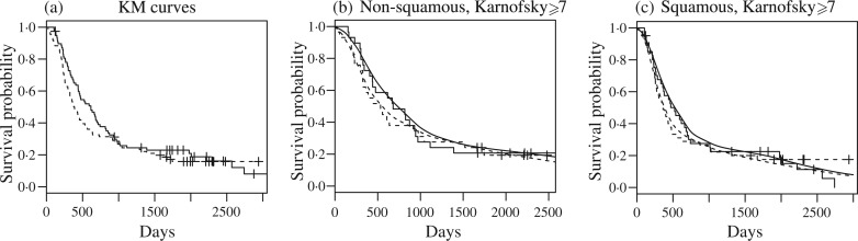
Lung cancer trial. (a) Kaplan–Meier estimates of survival functions. Solid lines refer to treatment and dashed lines refer to the control group. (b) and (c) The model-based estimates of survival curves arranged by cancer histology. For comparison, the corresponding Kaplan–Meier estimates are also included.

The prior is parameterized by α_ε = 4 for every ε. The kernels q_x in this case are multivariate normal densities with diagonal covariance matrix and the three standard deviations equal to 3.

As this example demonstrates the proposed multivariate Polya tree can easily be implemented for a moderate number of covariates. In fact, the computational effort of posterior inference scales only with the sample size, not with the number of covariates. Here the estimates of the survival curves have been obtained on the basis of 25 000 iterations of the proposed algorithm, after a burn in of 7000 iterations. The only concern limiting the number of covariates is the ability to define meaningful kernels to induce the desired correlation. For practical implementations, we see no problem with using the model with up to ten or so covariates.

Figure 4 summarizes some aspects of posterior inference under the proposed model. The model-based estimates identify crossing survival functions. The corresponding Kaplan–Meier curves are shown for comparison. Despite prior centring around the proportional hazards structure, posterior inference correctly identifies the intersecting curves. In contrast to the proportional hazards model, the proposed mpt model allows posterior inference to violate the structure of the prior centring family if the data so indicate.

6. Discussion

The construction of probability models for dependent random measures has been studied by several authors in recent years. Among these, MacEachern (1999) and De Iorio et. al. (2004) explore the idea of defining dependent random probability measures by means of an extension of the Dirichlet process mixture model while Dunson & Park (2008) discuss an extension of the stick-breaking representation.

The two main guiding principles in the proposed construction of dependent random probability measures are the need to specify prior distributions with a clear interpretation and the aim of constructing a probability model with large support.

One of the main strengths of the proposed approach is the use of marginal Polya tree priors, which allows one to restrict the model to continuous random distributions. Posterior inference under the finite multivariate Polya tree model allows easy interpretation as essentially a random histogram method. Some of the remaining limitations are computational challenges of higher dimensional extensions, requiring the manipulation of higher dimensional partitioning subsets, and the sensitivity of posterior inference on partitioning boundaries. The latter is greatly mitigated by the hierarchical extension of the multivariate Polya tree model to a mixture of multivariate Polya trees with a hyperprior for the centring model.

The multivariate beta process has interesting applications beyond the multivariate Polya tree model. The multivariate beta process provides a flexible construction to define dependent random probabilities indexed by covariates; the proposed approach can be generalized for defining dependent random vectors on a finite-dimensional simplex or dependent discrete random distributions. For example, it could be used to define priors for finite mixtures by formalizing a regression of mixture weights on covariates.

A natural continuation to the above line of research is the study of the asymptotic properties of Bayesian inferential procedures based on the proposed class of dependent random probability measures. We hope that the strict similarities of the multivariate Polya tree model with the tail free prior distributions could prove helpful in future research for exploring its asymptotic behaviour.

Appendix.

Proposition A1. Let α₀ and α₁ be two strictly positive real values. If

$$r_2^0=r_1^0={\alpha }_0(1-a),\hspace{0.17em}\hspace{0.17em}{r}_c^0={\alpha }_{0}a,\hspace{0.17em}\hspace{0.17em}{r}_2^1=r_1^1={\alpha }_1(1-a),\hspace{0.17em}\hspace{0.17em}{r}_c^1={\alpha }_{1}a,$$

where a ∈ (0, 1), and ( $G_1^0$, $G_2^0$, $G_1^1$, $G_2^1$, $G_c^0$, $G_c^1$) are independent gamma random variables with same scale parameter and shape parameters ( $r_1^0$, $r_2^0$, $r_1^1$, $r_2^1$, $r_c^0$, $r_c^1$), then the function

$$\rho (a)=\text{corr}\hspace{0.17em}\left(\frac{G_1^0+G_c^0}{G_1^0+G_c^0+G_1^1+G_c^1},\frac{G_2^0+G_c^0}{G_2^0+G_c^0+G_2^1+G_c^1}\right)$$

is monotone increasing.

Proof. The vector

$$\left(\frac{G_1^0}{G_1^0+G_2^0+G_1^1+G_2^1+G_c^0+G_c^1},\dots ,\frac{G_c^0}{G_1^0+G_2^0+G_1^1+G_2^1+G_c^0+G_c^1}\right)$$

is Dirichlet distributed with parameter ( $r_1^0$, $r_2^0$, $r_1^1$, $r_2^1$, $r_c^0$, $r_c^1$). Consider a Blackwell–McQueen random sequence {l_k}_k⩾1 from an urn with initial weights ( $r_1^0$, $r_2^0$, $r_1^1$, $r_2^1$, $r_c^0$, $r_c^1$) and colours ( $C_1^0$, $C_2^0$, $C_1^1$, $C_2^1$, $C_c^0$, $C_c^1$). Let S be the first ball from the Blackwell–McQeen urn whose colour belongs to the set ( $C_1^0$, $C_1^1$, $C_c^0$, $C_c^1$) and let V be the first ball, subsequent to S, whose colour belongs to the set ( $C_2^0$, $C_2^1$, $C_c^0$, $C_c^1$). Then

$$\begin{array}{ll}E\hfill & \left(\frac{G_1^0+G_c^0}{G_1^0+G_c^0+G_1^1+G_c^1}\frac{G_2^0+G_c^0}{G_2^0+G_c^0+G_2^1+G_c^1}\right)\hfill \\ \hfill & =\text{pr}\{S\in (C_1^0\cup C_c^0),V\in (C_2^0\cup C_c^0)\}\hfill \\ \hfill & =\sum _{m=1}^{\infty }\text{pr}\hspace{0.17em}\left\{\underset{k=1}{\overset{m-1}{\cap }}{l}_k\in (C_2^0\cup C_2^1),l_m\in (C_1^0\cup C_c^0)\right\}\hfill \\ \hfill & \hspace{0.17em}\hspace{0.17em}\hspace{0.17em}\hspace{0.17em}\times \text{pr}\hspace{0.17em}\left\{V\in (C_2^0\cup C_c^0)|\underset{k=1}{\overset{m-1}{\cap }}{l}_k\in (C_2^0\cup C_2^1),l_m\in (C_1^0\cup C_c^0)\right\}.\hfill \end{array}$$ (A1)

For each component of the sum, the first product term equals

$$p^{\prime }(a,m)=\frac{{\alpha }_0}{(2-a)({\alpha }_0+{\alpha }_1)+m-1}\prod _{k=1}^{m-1}\frac{(1-a)({\alpha }_0+{\alpha }_1)+k-1}{(2-a)({\alpha }_0+{\alpha }_1)+k-1}$$

and the second equals

$$p^{″}(a,m)=\left(\frac{{\alpha }_0}{{\alpha }_0+{\alpha }_1}\right)\hspace{0.17em}\left\{1-a\frac{a({\alpha }_0+{\alpha }_1)+1}{({\alpha }_0+{\alpha }_1)+m}\right\}+\left\{a\frac{{a\alpha }_0+1}{({\alpha }_0+{\alpha }_1)+m}\right\}.$$

The following inequalities can be verified with simple algebra. If a, a^* and a^** belong to the interval (0, 1) and a^** > a^*, then ∑_m⩾j p′(a^**, m) ⩽ ∑_m⩾j p′(a^*, m) for every j and, for every m, p″(a^**, m) > p″(a^*, m) and p″(a, m) > p″(a, m + 1). These inequalities and the equality ∑_m⩾1 p′(a^**, m) = ∑_m⩾j p′(a^*, m) imply that

$$\sum _{m=1}^{\infty }{p}^{\prime }(a**,m)p^{″}(a**,m)>\sum _{m=1}^{\infty }{p}^{\prime }(a*,m){p^{\prime }}^{\prime }(a*,m).$$

The last inequality completes the proof, indeed the two terms are equivalent to the expected value in (A1) under different parameterizations of $G_1^0$, …, $G_c^1$.

Proof of Proposition 1. For every i, let

$$\begin{array}{l}{G}_{x,x_i}^0=G[(z,y)\in X\times 𝕉:0<y<{\alpha }_0\text{min}\{q_{x_i}(z),q_x(z)\}],\\ G_{x\backslash x_i}^0=G\{(z,y)\in X\times 𝕉:0<y<{\alpha }_0{q}_x(z),y⩾{\alpha }_0{q}_{x_i}(z)\},\\ G_{x_i\backslash x}^0=G\{(z,y)\in X\times 𝕉:0<y<{\alpha }_0{q}_{x_i}(z),y⩾{\alpha }_0{q}_x(z)\}.\end{array}$$

We observe that $G(S_x^0)=G_{x,x_i}^0+G_{x\backslash x_i}^0$, $G(S_{x_i}^0)=G_{x,x_i}^0+G_{x_i\backslash x}^0$ and

$$E[{\{G(S_x^0)-G(S_{x_i}^0)\}}^2]=E\{{(G_{x\backslash x_i}^0-G_{x_i\backslash x}^0)}^2\}=2\text{var}(G_{x_i\backslash x}^0).$$

The hypotheses imply that ν{(z, y) ∈ X × 𝕉 : 0 < y < q_xi(z), q_x (z) > y} → 0, and it follows that var( $G_{x_i\backslash x}^0$) → 0. We can similarly define $G_{x,x_i}^1$, $G_{x\backslash x_i}^1$ and $G_{x_i\backslash x}^1$, and verify that $E[{\{G(S_x^1)-G(S_{x_i}^1)\}}^2]\to 0$. Finally, the convergences in mean square of {G( $S_{x_i}^0$)}_i⩾1 and {G( $S_{x_i}^1$)}_i⩾1 imply that, for every ε > 0, pr(| Y_xi − Y_x |> ε) → 0.

Proof of Proposition 2. For every $\epsilon \in {\cup }_{i=1}^{\infty }{\{0,1\}}^i$, E[𝒫_x{ $F_x^{-1}$(B_ε)}] = λ (B_ε), where λ denotes the Lebesgue measure. The same equality holds for the elements of the algebra of finite unions of B_ε sets. The class (B ⊆ (0, 1] : λ(B) = E[𝒫_x{ $F_x^{-1}$(B)}]) is monotone. The monotone class theorem implies that for every Borel subset B of (0, 1], E[𝒫_x{ $F_x^{-1}$(B)}] = λ(B). Finally, if a distribution p satisfies the equality p{ $F_x^{-1}$(B)} = λ(B) for every Borel subset B of (0, 1] then p = F_x.

Proof of Proposition 3. Proposition 1 implies that, for every $\epsilon \in {\cup }_{i=1}^{\infty }{\{0,1\}}^i$, the sequence 𝒫_xi{ $F_{x_i}^{-1}$ (B_ε)} (i = 1, 2 …) converges in probability to 𝒫_x{ $F_x^{-1}$(B_ε)}. Similarly, if a measurable set B belongs to the algebra generated by {B_ε; $\epsilon \in {\cup }_{i=1}^{\infty }{\{0,1\}}^i$}, then the random variables 𝒫_xi{ $F_{x_i}^{-1}$ (B)} converge in probability to 𝒫_x{ $F_x^{-1}$ (B)}. Let B ⊂ [0, 1] be a measurable set. Let B₁, B₂, …be an increasing sequence such that ∪_j⩾1 B_j = B and assume that, for every j ⩾ 1, the random variables 𝒫_xi{ $F_{x_i}^{-1}$ (B_j)} converge in probability to 𝒫_x{ $F_x^{-1}$ (B_j)}. We observe that, for every pair (i, j), 𝒫_xi{ $F_{x_i}^{-1}$ (B)} − 𝒫_xi{ $F_{x_i}^{-1}$ (B_j)} ⩾ 0 almost surely. We also observe that E[𝒫_xi{ $F_{x_i}^{-1}$ (B)} − 𝒫_xi{ $F_{x_i}^{-1}$ (B_j)}] = λ (B\B_j), where λ denotes the Lebesgue measure. It follows, using the Markov inequality, that, for every δ > 0 and ξ > 0, there exists m such that

$$\begin{array}{c}\text{pr}\hspace{0.17em}\left[|{𝒫}_x\{F_x^{-1}(B_m)\}-{𝒫}_x\{F_x^{-1}(B)\}|>\frac{\xi }{3}\right]<\frac{\delta }{3},\\ \text{pr}\left[|{𝒫}_{x_i}\{F_{x_i}^{-1}(B_m)\}-{𝒫}_{x_i}\{F_{x_i}^{-1}(B)\}|>\frac{\xi }{3}\right]<\frac{\delta }{3},\hspace{0.17em}\hspace{0.17em}\hspace{0.17em}\hspace{0.17em}\hspace{0.17em}\hspace{0.17em}\hspace{0.17em}i⩾1.\end{array}$$

Moreover, there exists k ⩾ 1 such that, for every j > k,

$$\text{pr}\hspace{0.17em}\left[|{𝒫}_{x_j}\{F_{x_j}^{-1}(B_m)\}-{𝒫}_x\{F_x^{-1}(B_m)\}|>\frac{\xi }{3}\right]<\frac{\delta }{3}.$$

For every j > k, pr[|𝒫_xj{ $F_{x_j}^{-1}$ (B)} − 𝒫_x{ $F_x^{-1}$ (B)}| > ξ] < δ. Similarly, if the sequence B₁, B₂, …decreases to B and, for every j ⩾1, the random variables 𝒫_xi{ $F_{x_i}^{-1}$ (B_j)} converge in probability to 𝒫_x{ $F_x^{-1}$ (B_j)}, then the sequence 𝒫_xi{ $F_{x_i}^{-1}$ (B)} converges in probability to 𝒫_x{ $F_x^{-1}$ (B)}. It follows, using the monotone class theorem, that for every Borel subset B ⊂ [0, 1] the sequence 𝒫_xi{ $F_{x_i}^{-1}$ (B)} converges in probability to 𝒫_x{ $F_x^{-1}$ (B)}.

Assume that the pair (a, b) satisfies c = F_x (a). The cumulative distribution functions F_xi and F_x are continuous. Therefore, the variables |𝒫_xi{(−∞, $F_{x_i}^{-1}$ (c)]} − 𝒫_x{(−∞, a]}| and |𝒫_xi{ $F_{x_i}^{-1}$ (0, c]} − 𝒫_x{ $F_{x_i}^{-1}$ (0, c]}| are almost surely identical. The random sequence |𝒫_xi{ $F_{x_i}^{-1}$ (0, c]} − 𝒫_x{ $F_x^{-1}$ (0, c]}| converges in probability to zero. Note that E[|𝒫_xi{(− ∞, $F_{x_i}^{-1}$ (c)]} − 𝒫_xi{−∞, a]}|] =|c − F_xi(a)| and |c − F_xi (a)|→ 0. It follows that the random sequences |𝒫_xi{(−∞, $F_{x_i}^{-1}$(c)]} − 𝒫_xi{(−∞, a]}| and |𝒫_xi{(−∞, a]} − 𝒫_x{(−∞, a]}| converge in probability to zero. Finally, through monotone class arguments and exploiting the convergence in total variation of {F_xi}_i⩾1 to F_x, we verify that, for every Borel subset B, the sequence 𝒫_xi(B) converges in probability to 𝒫_x(B).

Proof of Proposition 4. Assume that {Y_x}_x∈X ∼ mbp(α₀, α₁, Q). We prove that for every ξ > 0, for every m = 1, 2, …, for every distinct x₁, …, x_m ∈ X and a₁, …, a_m ∈ [0, 1] the event {|Y_xi − a_i | < ξ; i =1, …m} has strictly positive probability.

There exist strictly positive numbers ( $g_1^0$, $g_1^1$) such that | $\{g_1^0/(g_1^0+g_1^1)\}$ − a₁| < ξ/2. Given $G(S_{x_1}^0)=g_1^0$ and $G(S_{x_1}^1)=g_1^1$, there exist strictly positive numbers ( $g_2^0$, $g_2^1$) such that, if $G(S_{x_2}^0\backslash S_{x_1}^0)=g_2^0$ and $G(S_{x_2}^1\backslash S_{x_1}^1)=g_2^1$, then $|[G(S_{x_2}^1)/\{G(S_{x_2}^0)+G(S_{x_2}^1)\}]$ − a₂| < ξ/2. Similarly, for any fixed value of $G(S_{x_1}^1\cup S_{x_2}^1\cup \dots \cup S_{x_i}^1)$ and $G(S_{x_1}^0\cup S_{x_2}^0\cup \dots \cup S_{x_i}^0)$, there exist positive numbers ( $g_{i+1}^0$, $g_{i+1}^1$) such that, if $G\{S_{x_{i+1}}^0\backslash (S_{x_1}^0\cup \dots \cup S_{x_i}^0)\}=g_{i+1}^0$ and $G\{S_{x_{i+1}}^1\backslash (S_{x_1}^1\cup \dots \cup S_{x_i}^1)\}=g_{i+1}^1$, then $|[G(S_{xi+1}^1)/\{G(S_{x_{i+1}}^0)+G(S_{x_{i+1}}^1)\}]$ − a_i+1|< ξ/2. The quantities $\nu (S_{x_1}^0)$, $\nu (S_{x_1}^1)$, $\nu (S_{x_2}^0\backslash S_{x_1}^0),\dots ,\nu \{S_{x_m}^1\backslash (S_{x_1}^1\cup \dots \cup S_{x_{m-1}}^1)\}$ are strictly positive, indeed {q_x}_x∈X is a location family of unimodal densities. It follows that the density function of [ $G(S_{x_1}^0)$, $G(S_{x_1}^1)$, $G(S_{x_2}^0\backslash S_{x_1}^0),\dots ,G\{S_{x_m}^1\backslash (S_{x_1}^1\cup \dots \cup S_{x_{m-1}}^1)\}$] in an adequate neighbourhood of ( $g_1^0$, $g_1^1,\dots ,g_m^1)$ is strictly positive. This fact proves our assertion.

For every positive ξ and every integer j the event

$$\left\{|{𝒮}_i\left(F_{x_i}^{-1}\hspace{0.17em}(\frac{l}{2^j},\frac{l+1}{2^j}\right])-{𝒫}_{x_i}\hspace{0.17em}\left(F_{x_i}^{-1}\hspace{0.17em}(\frac{l}{2^j},\frac{l+1}{2^j}]\right)|<\xi ;l⩽(2^j-1),i=1,\dots ,m\right\}$$

has strictly positive probability. Finally, for any positive δ and partition (V₁, …, V_k) constituted of intervals, the absolute continuity hypothesis S_i ≪ F_xi ≪ λ, where λ denotes the Lebesgue measure, implies that, if j and ξ are suitably chosen, then this event becomes a subset of {|𝒮_i (V_l) − 𝒫_xiV_l)| < δ; l = 1, …, k, i = 1, …, m}.

References

- Berger JO, Guglielmi A. Bayesian testing of a parametric model versus nonparametric alternatives. J Am Statist Assoc. 2001;96:174–84. [Google Scholar]
- Berman M. A class of isotropic distributions in Rn and their characteristic functions. Pac J Math. 1978;78:1–9. [Google Scholar]
- Blackwell D, MacQueen JB. Ferguson distributions via Polya urn schemes. Ann Statist. 1973;1:353–5. [Google Scholar]
- De Iorio M, Muller P, Rosner GL, MacEachern S. An ANOVA model for dependent random measures. J Am Statist Assoc. 2004;99:205–15. [Google Scholar]
- Doksum K. Tailfree and neutral random probabilities and their posterior distributions. Ann Prob. 1974;2:183–201. [Google Scholar]
- Dunson DB, Park BK. Kernel stick-breaking processes. Biometrika. 2008;95:307–23. doi: 10.1093/biomet/asn012. [DOI] [PMC free article] [PubMed] [Google Scholar]
- Dunson DB, Pillai N, Park BK. Bayesian density regression. J. R. Statist. Soc. B. 2007;69:163–83. [Google Scholar]
- Ferguson TS. Prior distributions on spaces of probability measures. Ann Statist. 1974;4:615–29. [Google Scholar]
- Gneiting T. Radial positive definite functions generated by Euclid’s hat. J Mult Anal. 1999;69:88–19. [Google Scholar]
- Hanson T. Inference for mixtures of finite Polya tree models. J Am Statist Assoc. 2006;101:1548–65. [Google Scholar]
- Hanson T, Johnson W. Modeling regression error with a mixture of Polya trees. J Am Statist Assoc. 2002;97:1020–33. [Google Scholar]
- Hjort NL. Nonparametric Bayes estimators based on Beta processes in models for life history data. Ann Statist. 1990;18:1259–94. [Google Scholar]
- Lad T, Rubinstein L, Sadeghi A. The benefit of adjuvant treatment for resected locally advanced non-small-cell lung cancer. J Clin Oncol. 1988;6:9–17. doi: 10.1200/JCO.1988.6.1.9. [DOI] [PubMed] [Google Scholar]
- Lavine M. Some aspects of Polya tree distributions for statistical modelling. Ann Statist. 1992;20:1222–35. [Google Scholar]
- Lavine M. More aspects of Polya tree distributions for statistical modelling. Ann Statist. 1994;22:1161–76. [Google Scholar]
- MacEachern S. ASA Proc Sec Bayesian Statist Sci. Alexandria, VA: American Statistical Association; 1999. Dependent nonparametric processes; pp. 50–5. [Google Scholar]
- Mauldin RD, Sudderth WD, Williams SC. Polya trees and random distributions. Ann Statist. 1992;20:1203–21. [Google Scholar]
- Mittal Y. A class of isotropic covariance functions. Pac. J. Math. 1976;64:517–38. [Google Scholar]
- Nadarajah S, Kotz S. Some bivariate beta distributions. Statistics. 2005;39:457–66. [Google Scholar]
- Nieto-Barajas LE, Walker SG. Gibbs and autoregressive processes. Statist Prob Lett. 2007;77:1479–85. [Google Scholar]
- Olkin I, Liu R. A bivariate beta distribution. Statist Prob Lett. 2003;62:407–12. [Google Scholar]
- Piantadosi S. Clinical Trials: A Methodologic Perspective. New York: Wiley; 1997. [Google Scholar]
- Raftery AE, Lewis SM. How many iterations in the Gibbs sampler? In: Bernardo JM, Berger JO, Dawid AP, Smith AFM, editors. Bayesian Statist 4. Oxford: Oxford University Press; 1992. pp. 763–73. [Google Scholar]
- Walker S, Mallick BK. A Bayesian semiparametric accelerated failure time model. Biometrics. 1999;55:477–83. doi: 10.1111/j.0006-341x.1999.00477.x. [DOI] [PubMed] [Google Scholar]
- Walker S, Muliere P. A bivariate Dirichlet process. Statist Prob Lett. 2003;64:1–7. [Google Scholar]