DataHigh: Graphical user interface for visualizing and interacting with high-dimensional neural activity

Abstract

The activity of tens to hundreds of neurons can be succinctly summarized by a smaller number of latent variables extracted using dimensionality reduction methods. These latent variables define a reduced-dimensional space in which we can study how population activity varies over time, across trials, and across experimental conditions. Ideally, we would like to visualize the population activity directly in the reduced-dimensional space, whose optimal dimensionality (as determined from the data) is typically greater than 3. However, direct plotting can only provide a 2D or 3D view. To address this limitation, we developed a Matlab graphical user interface (GUI) that allows the user to quickly navigate through a continuum of different 2D projections of the reduced-dimensional space. To demonstrate the utility and versatility of this GUI, we applied it to visualize population activity recorded in premotor and motor cortices during reaching tasks. Examples include single-trial population activity recorded using a multi-electrode array, as well as trial-averaged population activity recorded sequentially using single electrodes. Because any single 2D projection may provide a misleading impression of the data, being able to see a large number of 2D projections is critical for intuition- and hypothesis-building during exploratory data analysis. The GUI includes a suite of additional interactive tools, including playing out population activity timecourses as a movie and displaying summary statistics, such as covariance ellipses and average timecourses. The use of visualization tools like the GUI developed here, in tandem with dimensionality reduction methods, has the potential to further our understanding of neural population activity.

I. Introduction

A major challenge in systems neuroscience is to interpret the activity of large populations of neurons, which may be recorded either simultaneously or sequentially [1]. One approach for characterizing the activity of tens to hundreds of neurons is to extract a smaller number of latent variables that can succinctly summarize the population activity. This approach has been applied to study the motor system [2], olfactory system [3], visual system [2], working memory in prefrontal cortex [4], and rule learning in prefrontal cortex [5]. Dimensionality reduction methods to extract these latent variables include principal component analysis (PCA) [3], [4], factor analysis (FA) [6], Gaussian-process factor analysis (GPFA) [7], and locally-linear embedding (LLE) [3].

The basic setup is to first define an n-dimensional space, where each axis represents the firing rate of one of the n neurons in the population. A dimensionality reduction method is then applied to the n-dimensional population activity to determine the optimal number, r, of latent variables needed to adequately capture the population activity (r < n), as well as the relationship between the latent variables and the population activity. These latent variables define a reduced r-dimensional space in which we can study how the population activity varies over time, across trials, and across experimental conditions. Ideally, we would like to visualize the latent variables directly in the r-dimensional space. However, the optimal number r of latent variables, as determined from the data, is typically greater than three [4], [6], [7] and direct plotting can only provide a 2D or 3D view. A common approach is to visualize a small number of 2D projections, obtained by specifying some cost function, which may give a misleading impression of the data.

To address this limitation, we developed an interactive graphical user interface (GUI), called DataHigh, in Matlab for visualizing a continuum of 2D projections. The user first applies a dimensionality reduction method of their choice to the neural activity, then passes the reduced-dimensional data to DataHigh for visualization. We found DataHigh to be a valuable tool for building intuition about the population activity and for hypothesis generation. Although high-dimensional visualization is a challenge across many scientific fields, we designed DataHigh explicitly for neural data analysis. DataHigh is versatile and can be used to study population activity recorded either simultaneously (using multi-electrode arrays) or sequentially (using conventional single electrodes). It can be applied to visualize i) the trial-to-trial variability of population activity taken in a single, predefined time bin (termed neural state), ii) single-trial population activity timecourses (termed neural trajectories), or iii) trial-averaged neural trajectories. Sections II and III describe the design and features of DataHigh. Section IV shows examples of using DataHigh to analyze neural population activity.

II. Rotating a 2D projection plane

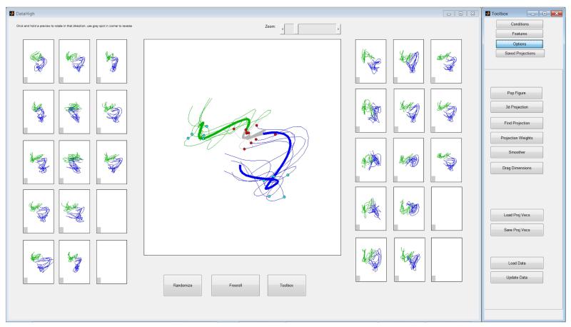
The main interface of DataHigh (Fig. 1) allows the user to smoothly rotate a 2D projection plane in the r-dimensional space. The goal is to provide the minimum set of “knobs” that allow the user to achieve all possible rotations within the r-dimensional space. We first describe the idea of our approach, then the mathematical implementation. We begin with two arbitrary orthonormal r-dimensional vectors, v₁ and v₂, which define the horizontal and vertical axes, respectively, of a 2D projection plane. To rotate the projection plane, we fix one vector v₁, while rotating the other vector v₂. To maintain orthogonality, v₂ must rotate in the (r−1) dimensional orthogonal space of v₁. In this space, any rotation of v₂ can be fully specified by (r−2) angles. Thus, we provide the user with (r−2) knobs (right panels in Fig. 1) to rotate v₂ while keeping v₁ fixed. Each panel shows a preview of the resulting 2D projection if v₂ were rotated by 180° in a particular rotation plane. The user can click and hold on a particular preview panel, which continuously updates the central panel as v₂ is smoothly rotated in that plane. Similarly, we can fix v₂ and rotate v₁, which yields an additional (r−2) preview panels (left panels in Fig. 1). Note that the r-dimensional data are centered before projection.

Fig. 1.

Main interface for DataHigh. Central panel: 2D projection of 15D single-trial neural trajectories extracted using GPFA from population activity recorded in premotor cortex during a standard delayed-reaching task for two different reach targets (blue and green) [7]. Dots indicate time of target onset (red) and go cue (cyan). Gray indicates baseline activity. Preview panels (left and right of central panel): clicking and holding on a preview panel rotates one of the two projection vectors for the central panel. Toolbar (far right) accesses features described in Section III.

Mathematically, we first use the Gram-Schmidt process to find a set of (r−1) orthonormal vectors spanning the orthogonal space of v₁; these vectors define the columns of $𝘘\in {ℝ}^{r\times (r-1)}$. We also define a rotation matrix $R_i\left(\theta \right)\in {ℝ}^{(r-1)\times (r-1)}$, which rotates an (r−1) dimensional vector by θ degrees in the ith rotation plane.

$$R_i\left(\theta \right)=\left[\begin{array}{cccc}\hfill I_{i-1}\hfill & \hfill \hfill & \hfill \hfill & \hfill \hfill \\ \hfill \hfill & \hfill \cos \left(\theta \right)\hfill & \hfill -\sin \left(\theta \right)\hfill & \hfill \hfill \\ \hfill \hfill & \hfill \sin \left(\theta \right)\hfill & \hfill \cos \left(\theta \right)\hfill & \hfill \hfill \\ \hfill \hfill & \hfill \hfill & \hfill \hfill & \hfill I_{r-i-2}\hfill \end{array}\right],$$ (1)

where I_p is a p × p identity matrix and i = 1, …, r−2. To rotate v₂ by θ degrees in the ith rotation plane, we compute

$${\mathbf{v}}_2^{\mathrm{new}}=𝘘R_i\left(\theta \right){𝘘}^T{\mathbf{v}}_2^{\mathrm{old}}.$$ (2)

The neural trajectories shown in Fig. 1 are 15-dimensional, leading to the use of 2 · (r−2) = 26 preview panels. At present, DataHigh can support dimensionalities up to r = 17 (30 preview panels), which we found to be large enough for most current analyses, yet small enough to have all preview panels displayed simultaneously on a standard monitor. For r > 17, DataHigh applies PCA to the data and retains the top 17 PCA dimensions for visualization. Alternatively, DataHigh can be easily extended to have a larger number of preview panels.

III. DataHigh features

In addition to the continuous rotation of a 2D projection plane, DataHigh offers a suite of additional features that are useful for exploratory data analysis:

• Freeroll continuously rotates the 2D projection plane in a random fashion without user intervention. The GUI repeatedly “clicks and holds” on a random preview panel for a random period of time.

• Conditions allows the user to selectively display any subset of the experimental conditions in the dataset. The user is given the option to recenter the data based on the updated set of experimental conditions.

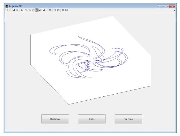
• 3D projection uses the current 2D projection, along with a randomly-chosen third projection vector, to allow visualization in Matlab’s built-in 3D viewer (Fig. 2).

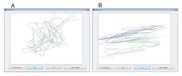
• Find projection displays the static 2D projections found by PCA or linear discriminant anaysis (LDA) (Fig. 3).

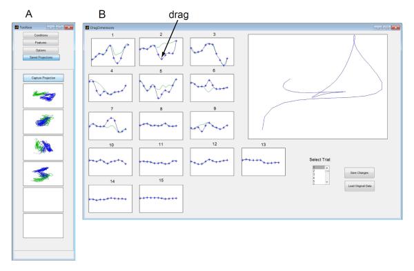
• Capture saves the current 2D projection by adding its thumbnail image to the list of saved projections (Fig. 4A). A projection can be loaded simply by clicking on its thumbnail image. The user can also manually specify and save the values of v₁ and v₂, as well as save a 2D projection as a Matlab figure.

• Weights displays the elements of v₁ and v₂ as bar graphs.

• Evolve displays a movie of the neural trajectories playing out together over time. The movie may be saved for external viewing.

• Drag trajectory plots each of the r dimensions of a neural trajectory versus time (Fig. 4B). The user can “perturb” the trajectory by dragging any of the points in the dimension versus time plots and see its effect in the 2D projection. The perturbed trajectory can then be sent to the central panel (Fig. 1) for further inspection.

• Smoother convolves the input data with a Gaussian kernel for temporal smoothing. It is intended for use with input data that have not already been smoothed (e.g., raw spike counts or trial-averaged spike counts). The smoothing kernel width is chosen by a scroll bar, and the plots are updated immediately.

• Additional features for neural trajectories: display trial-averaged trajectories for each experimental condition and plot task epoch boundaries with colored dots (Fig. 1).

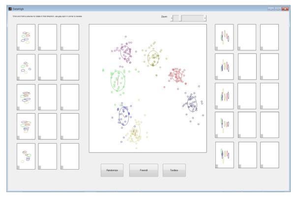
• Additional features for neural states: for each experimental condition, plot cluster mean, covariance ellipse, and first principal component direction (Fig. 5).

Fig. 2.

A 3D projection of trial-averaged neural trajectories during reaching movements. Each trajectory corresponds to one reach condition.

Fig. 3.

Static 2D projections found by standard methods, A: PCA and B: LDA, when applied to the data shown in Fig. 1. In contrast, DataHigh (Fig. 1) can find a dynamic 2D projection in which the trajectories splay out over time and are largely non-overlapping for different reach conditions.

Fig. 4.

DataHigh features. A: Capture projection, B: Drag trajectory.

Fig. 5.

Trial-to-trial variability of neural state during reach planning. Each dot corresponds to one trial and is colored according to reach target. For each cluster, the user can choose to display the one standard deviation ellipse and/or the direction of greatest trial-to-trial variability (red lines).

IV. Data analysis examples

We demonstrate here a few examples of the utility of DataHigh for exploratory data analysis.

Trial-to-trial variability of neural state

For each trial, we first took the spike counts across n = 61 simultaneously-recorded neurons in a single, predefined time bin during the delay period in a standard delayed-reaching task [6]. FA was then applied to reduce the dimensionality of each 61D vector of spike counts to a 7D vector of latent factors (a neural state). The FA parameters were fit using trials of all reach targets together, and the optimal latent dimensionality (r = 7) was determined using cross-validation. We used DataHigh to visualize the 7D latent factors (Fig. 5). By rotating the 2D projection plane, we can study the relative placement of the clusters, as well as the trial-to-trial variability. For each cluster, a red line represents the 2D projection of a unit vector pointing in the direction of greatest trial-to-trial variability in the 7D latent space. The length of the red line indicates the extent to which the direction of greatest variability in the 7D space aligns with the 2D projection plane. Note that the red lines need not align with the direction of greatest variability as seen in the 2D projection (i.e., each red line need not align with the major axis of the corresponding ellipse). This underscores the danger of drawing conclusions from any individual 2D projection, as well as the need for looking at many 2D projections using DataHigh.

Single-trial neural trajectories

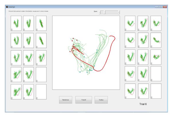
It is often difficult to find an informative 2D projection of high-dimensional data. Two common approaches are PCA (Fig. 3A) and LDA (Fig. 3B), which yield projections in which the trajectories look like “spaghetti”. Using DataHigh, we can quickly search a large number of 2D projections to find projections in which the trajectories splay out over time and are mostly non-overlapping for different experimental conditions (Fig. 1). We also find DataHigh to be useful for identifying outlying trials and studying their relationship with the non-outlying trials (Fig. 6). The DataHigh interface allows the user to highlight any trajectory by clicking on it, change the color of the trajectory on the fly, and save this change to the Matlab data structure.

Fig. 6.

An outlying trial (red trace) can be easily identified by rotating the 2D projection plane.

Trial-averaged neural trajectories

DataHigh can also be used to study trial-averaged neural trajectories obtained from sequentially-recorded neurons. Fig. 2 shows rotational structure in the movement-related neural activity during arm reaches [8]. Each trajectory corresponds to the trial-averaged activity of 118 neurons recorded in motor cortex for one reach condition. DataHigh can be used to find the planes in which rotational structure is present in the data, as well as provide insight about the population activity in non-rotational planes.

V. Discussion

To date, the visualization of high-dimensional neural population activity has largely relied on a small number of 2D projections. If the features of interest of the neural activity are known in advance, one can specify a cost function to find a 2D projection that illustrates those features. However, in exploratory data analysis, the key features may not be known in advance, and it is easy to miss such features by looking at a small number of 2D projections. DataHigh allows for an “unbiased” exploration of neural population activity by displaying a large number of 2D projections in a short amount of time. This can be useful not only for triaging large datasets and identifying outlying trials, but also for developing scientific hypotheses about the data, which can then be tested quantitatively. In addition to visualizing latent variables extracted by a dimensionality reduction method (r-dimensional), DataHigh can also be used to visualize raw population spike counts (n-dimensional). We have put substantial effort into minimizing DataHigh’s response latency to enhance the user’s interactive experience. We plan to extend DataHigh to incorporate built-in dimensionality reduction methods for neural data. The software can be downloaded from http://users.ece.cmu.edu/~byronyu/software.

References

- [1].Stevenson IH, Kording KP. How advances in neural recording affect data analysis. Nat Neurosci. 2011 Feb;14(2):139–42. doi: 10.1038/nn.2731. [DOI] [PMC free article] [PubMed] [Google Scholar]
- [2].Churchland MM, Yu BM, Cunningham JP, Sugrue LP, Cohen MR, Corrado GS, Newsome WT, Clark AM, Hosseini P, Scott BB, Bradley DC, Smith MA, Kohn A, Movshon JA, Armstrong KM, Moore T, Chang SW, Snyder LH, Lisberger SG, Priebe NJ, Finn IM, Ferster D, Ryu SI, Santhanam G, Sahani M, Shenoy KV. Stimulus onset quenches neural variability: a widespread cortical phenomenon. Nat Neurosci. 2010 Mar;13(3):369–78. doi: 10.1038/nn.2501. [DOI] [PMC free article] [PubMed] [Google Scholar]
- [3].Stopfer M, Jayaraman V, Laurent G. Intensity versus identity coding in an olfactory system. Neuron. 2003 Sep;39(6):991–1004. doi: 10.1016/j.neuron.2003.08.011. [DOI] [PubMed] [Google Scholar]
- [4].Machens CK, Romo R, Brody CD. Functional, but not anatomical, separation of “what” and “when” in prefrontal cortex. J Neurosci. 2010 Jan;30(1):350–60. doi: 10.1523/JNEUROSCI.3276-09.2010. [DOI] [PMC free article] [PubMed] [Google Scholar]
- [5].Durstewitz D, Vittoz NM, Floresco SB, Seamans JK. Abrupt transitions between prefrontal neural ensemble states accompany behavioral transitions during rule learning. Neuron. 2010 May;66(3):438–48. doi: 10.1016/j.neuron.2010.03.029. [DOI] [PubMed] [Google Scholar]
- [6].Santhanam G, Yu BM, Gilja V, Ryu SI, Afshar A, Sahani M, Shenoy KV. Factor-analysis methods for higher-performance neural prostheses. J Neurophysiol. 2009 Aug;102(2):1315–30. doi: 10.1152/jn.00097.2009. [DOI] [PMC free article] [PubMed] [Google Scholar]
- [7].Yu BM, Cunningham JP, Santhanam G, Ryu SI, Shenoy KV, Sahani M. Gaussian-process factor analysis for low-dimensional single-trial analysis of neural population activity. J Neurophysiol. 2009 Jul;102(1):614–35. doi: 10.1152/jn.90941.2008. [DOI] [PMC free article] [PubMed] [Google Scholar]
- [8].Churchland MM, Cunningham JP, Kaufman MT, Ryu SI, Shenoy KV. Cortical preparatory activity: representation of movement or first cog in a dynamical machine? Neuron. 2010 Nov;68(3):387–400. doi: 10.1016/j.neuron.2010.09.015. [DOI] [PMC free article] [PubMed] [Google Scholar]