

Abstract
In optical coherence tomography (OCT) and ultrasound, unbiased Doppler frequency estimators with low variance are desirable for blood velocity estimation. Hardware improvements in OCT mean that ever higher acquisition rates are possible, which should also, in principle, improve estimation performance. Paradoxically, however, the widely used Kasai autocorrelation estimator’s performance worsens with increasing acquisition rate. We propose that parametric estimators based on accurate models of noise statistics can offer better performance. We derive a maximum likelihood estimator (MLE) based on a simple additive white Gaussian noise model, and show that it can outperform the Kasai autocorrelation estimator. In addition, we also derive the Cramer Rao lower bound (CRLB), and show that the variance of the MLE approaches the CRLB for moderate data lengths and noise levels. We note that the MLE performance improves with longer acquisition time, and remains constant or improves with higher acquisition rates. These qualities may make it a preferred technique as OCT imaging speed continues to improve. Finally, our work motivates the development of more general parametric estimators based on statistical models of decorrelation noise.
Index Terms: Cramer–Rao bound (CRB), Doppler optical coherence tomography, Doppler ultrasound, frequency estimation, maximum likelihood estimation (MLE)
I. Introduction
IN RECENT years, Doppler optical coherence tomography (OCT) has become an invaluable tool in blood velocity estimation [1], [2] and promises to be important for absolute blood flow quantification [3]. Many authors have provided valuable insight into Doppler frequency estimation in OCT [4]–[6], sonar [7], and ultrasound [8]–[11], including work that applied estimation theory to this problem [12]. One commonly used estimator, an autocorrelation method, was derived by Kasai [8] in 1985, during the era of analog electronics for use in continuous wave and pulse-echo Doppler ultrasound [13]–[15]. The Kasai estimator [8] has been widely used in Doppler frequency estimation [16] and has been ported for use in Doppler OCT. It is a fast and simple algorithm, with wide applicability due to its nonparametric nature.
On the other hand, it is known that the Kasai estimator is not statistically optimal in the sense of estimator mean squared error (MSE) and variance [17]. Since it was derived and first implemented with analog electronics, with most signal processing becoming digital nowadays, it is worthwhile to reevaluate the suitability of this technique in the discrete domain. In addition, Schmoll et al.[18] have noticed an undesirable feature of the discretized Kasai estimator: that increasing the acquisition rate decreases the estimator performance. In practice, the time between samples is sometimes increased in order to lower the estimator variance [18]. However, this clearly represents an undesirable feature, as this necessarily reduces the maximum measurable frequency. Discarding data in this manner negates the advantages of hardware advances towards higher acquisition rates [19].
In this paper, we first present a theoretical analysis and experimental verification to evaluate the performance of the Kasai estimator compared with the maximum likelihood estimator (MLE). We compare these estimators against the Cramer–Rao lower bound (CRLB), which indicates the theoretical best performance of an unbiased estimator. While ad hoc estimators may provide reasonable performance under practical situations, they may not be optimal. Maximum likelihood estimation (a parametric method) has the advantages of asymptotic efficiency, consistency and unbiasedness [17]. MLEs can closely match the CRLB, for moderate data lengths and signal-to-noise ratios (SNRs). Hence we propose MLEs as better alternatives to the Kasai estimator. The tradeoff, however, is that parametric estimators are more susceptible to outliers and violations of model assumptions [20], [21]. Parametric estimators may also be more computationally complex. Despite these limitations, they are better suited to take advantage of advances in computational power and improvements in OCT acquisition speed.
After a detailed discussion on the Kasai estimator, we describe a simple additive white Gaussian noise model for the Doppler OCT signal. By providing mathematical derivations of the MLE under these assumptions, we prove that the position of the peak of the power spectral density is the MLE for the Doppler frequency. From our model, we also derive the CRLB via an appropriate Fisher information matrix, and discuss the MLE’s limitations. This is done in the spirit of discrete-time signal processing, in contrast to the continuous-time analysis of [12]. Moreover, we show, through simulations, that the Kasai estimator is statistically suboptimal as determined by the standard performance metrics of estimator bias, variance, and efficiency. In addition, we examine the scaling properties of the Kasai autocorrelation estimator and the MLE with acquisition rate. We demonstrate that the MLE performance improves with acquisition time and remains constant or improves with acquisition rate. We conclude by highlighting the relative advantages of these estimators and point the direction for further improvements in algorithm development, with a brief discussion on the effects of multiplicative decorrelation noise on these estimators.
II. Kasai Estimator
Kasai derived an estimator [8] to calculate Doppler shifts of continuous wave ultrasound signals. The motivation was to deduce the Doppler frequency from the autocorrelation function. The most intuitive and direct way to measure the rate of rotation of a complex phasor is to measure the change over a small known time interval. One can integrate repeated measurements of the change to obtain a more precise estimate. The Kasai estimator essentially performs an integral of the phase changes to obtain an autocorrelation function, from which the average Doppler frequency is obtained. It can be seen, by the Wiener–Khinchin Theorem [22]–[24], that the Kasai autocorrelation estimate is analogous to the mean of the power spectrum. It is a nonparametric estimator in the sense that no assumption is made on the noise statistics.
A. Expression
Kasai [8] derived an estimator for the Doppler shift by finding the mean value of the angular frequency, Ω (see Table I), from the power spectrum P (Ω)
| (1) |
However, this form is not conducive to easy computation. From the Wiener–Khinchin Theorem, one can determine this in the time domain
| (2) |
While Kasai proposed this estimator for analog signals, it is now often utilized in its discrete form. To compute this, one would estimate the one-step autocorrelation function by
| (3) |
where sn is the signal acquired at the nth time instance. If its phase is given by ϕ(Δt) = ∠[R̂(Δt)] then one can estimate the mean angular frequency in (2) by dividing the phase subtended (indicated by the wedge signal, ∠) by the time elapsed Δt. This is the same as the rate of change in phase, ϕ̇(0), at time zero
| (4) |
| (5) |
This is a two-step estimation process. First, one estimates the autocorrelation function. Second, from the autocorrelation function at unit lag, one estimates the phase velocity. As the effects of noise were not considered in the derivation, and the autocorrelation function was assumed to be equal to its estimate, the Kasai autocorrelation estimate of frequency is ad hoc, and optimality was not considered.
Table I.
Some Frequently Used Symbols
| Symbol | Meaning |
|---|---|
| Ω | Analog Doppler frequency |
| R | Discrete/continuous autocorrelation function |
| T | Total acquisition time |
| N | Total number of data points |
| Δt | T/N |
| ∠ | Complex argument |
| r | Reflectance |
| ϕr | Phase of reflectance |
B. Advantages and Drawbacks
The Kasai estimator is computationally simple, with few operations: addition, multiplication and an arctangent. It can therefore be implemented in real-time easily and cheaply with very simple analog or digital electronics. However, these benefits are now largely secondary with the present state of computational capabilities.
As no assumptions are made about the noise statistics, the Kasai estimator also has a wider applicability than a parametric method such as the MLE. As it is nonparametric, a priori knowledge of the noise statistics is not utilized, which means the estimator will probably be nonoptimal. We show in our simulations (Section V) that the Kasai estimator does not achieve the CRLB for realistic SNRs.
III. Maximum Likelihood Estimator
The MLE is consistent, asymptotically unbiased, and asymptotically efficient [17]. Here, we show that the MLE for frequency is equal to the position of peak of the power spectral density. As the MLE is a parametric estimation technique, a full derivation requires a statistical noise model.
A. Model
Consider a stationary OCT beam focused at a single location. We are interested in the time evolution of the complex reflectance of this region of interest. We represent the signal as the sum of a rotating phasor and an additive white Gaussian noise (AWGN) component. The magnitude of the phasor is determined by the amplitude of backscattering, and in our discussion, is given by |r|. Red blood cells are the major backscatterer in blood, although platelets and white blood cells may also be present. In reality, so-called “decorrelation noise” will always be present, as one red blood cell is replaced by another with a different scattering amplitude and phase. Vakoc et al.[25] have shown that signal decorrelation is related to the Gaussian profile of an OCT beam. Accounting for decorrelation would lead to a more complicated noise model and MLE, but could potentially lead to more accurate estimates.
As a parametric method, the MLE is asymptotically optimal for the assumed noise model. Here, we examine the simplest noise model (additive, white Gaussian noise) for the OCT signal for the purposes of estimator comparison. This model is commonly used for the OCT signal, although more accurate decorrelation noise models are available [25], [26]. If the model is incorrect, the performance and accuracy of the estimator are uncertain [20], [21].
If sn is a single data point at time instance n, we represent the Doppler OCT data for measuring flow velocity as
| (6) |
Here, |r| exp(jϕr) is the unknown complex constant reflectance, and . All phase accumulated from backscattering and propagation are incorporated into ϕr. We wish to estimate the Doppler frequency, Ω, from the signal. The time between measurements is Δt = T/N, where T is the total acquisition time and N is the total number of samples. The discrete time instances are indexed by n. The additive noise is given by zn, which is circularly symmetric complex Gaussian, and independent identically distributed (i.i.d.). This means that each of the real and imaginary parts of zn are Gaussian and independent with variance σ2.
B. Derivation of Maximum Likelihood Estimator—Peak of Spectrum
From this model, as expressed in (6), we can calculate the likelihood of obtaining a measured signal. If s1 is a single measured datum, then each of the real and imaginary parts of the complex residual, s1 − |r| exp[j(ΩΔt + ϕr)], will have a Gaussian distribution with zero mean and variance σ2. Hence, the likelihood is given by
| (7) |
where x1 = Re [s1] is the real part of the signal and y1 = Im [s1] is the imaginary part. By grouping the N datum together, the log-likelihood function for the data can then be written in the form
| (8) |
The first term is a constant, and the second term can be written as
the last term of which is the real part of inverse discrete Fourier transform of { }. Given our estimated parameter vector θ̂ = (Ω̂, ϕ̂R)T
| (9) |
When performing maximum likelihood estimation, the data {s1,s2, …,sN }, the number of data points, N, and the total acquisition time, T, are known. We wish to find the values of Ω and ϕr that give the largest value for the likelihood function, derived assuming the noise model in (6). The MLE Ω̂MLE is obtained by choosing the values of the Doppler frequency, Ω, and reflectance phase, ϕr, that maximizes the real part of the inverse DFT of the complex conjugate of the signal. To maximize the expression in (9), ϕr is chosen so that the expression in curly brackets is real. Hence one may proceed to estimate the Doppler frequency Ω without estimating ϕr by finding the value of Ω that maximizes the absolute value of the DFT of the signal. This is the location of the peak of the power spectral density (PSD), as shown in Fig. 1, and can be found with established nonlinear search algorithms [27].
Fig. 1.
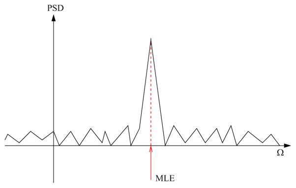
MLE for Doppler frequency is the location of the peak of the power spectral density.
C. Advantages and Drawbacks
The advantages of the MLE include asymptotic efficiency, consistency and asymptotic unbiasedness. However, its drawbacks include general problems with tractability, complexity, uniqueness [20], [21], and that optimality properties and unbiasedness may not apply for small samples. Tractability is not a problem here as we can perform a simple one-dimensional nonlinear search to locate the peak in our spectra. The computational complexity is low for a simple noise model, but may not be so for decorrelation noise. For a spectrum with a single peak, uniqueness does not pose a problem, but if static scattering is present, either clutter rejection [28]–[30] should be performed or a static clutter component should directly be incorporated into the parametric estimation. In our earlier work, we performed high-pass filtering [3] to remove the static scattering component of the OCT signal. For our simulation and flow phantom experiments in this paper, this was not required as the dynamic scattering components dominated.
Though MLE techniques can deliver asymptotically accurate and precise Doppler frequency estimates, they require more computation. The Kasai estimator only uses arithmetic operations and an arctangent operation. The MLE, as implemented in this paper, requires an FFT, which is
 (N log N). More generally, the MLE can be implemented with nonlinear search algorithms. In our experiments, shown in Fig. 8, the MLE took roughly five times longer than the Kasai estimate. The computation of color Doppler maps took less than a few seconds on a modern desktop computer using parallelized Matlab. Hence we believe that the MLE, with optimization or use of GPUs, can be used in real-time imaging.
Fig. 8.
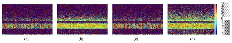
Color Doppler maps, with dimensions of 512 by 100, generated using the Kasai [(a), (b)] and AWGN ML [(c), (d)] estimators. The flow rate was 0.1 ml.hr−1, using intralipid-10% at a 16° incline, with a 10 dB SNR. Scanning was done at a fixed location. The x-axis is a time axis. The line scan rate was 47 kHz, and estimates were made with 4 [(a), (c)] and 16 [(b), (d)] data points, respectively, corresponding to acquisition times of 0.09 and 0.34 ms. These represent two of the conditions shown in Fig. 7(c) and (d). The variances of the Kasai estimator were 4.02 × 10⁷ rad2.s−2 (76.0 dB) and 3.12 × 10⁶ rad2.s−2 (64.9 dB), respectively. For the MLE, zero padding was used to increase the FFT lengths by 256. For acquisition times of roughly 0.17 ms and below the MLE outperforms the Kasai estimator. The variances of the ML estimates were 2.83 × 10⁷ rad2.s−2 (74.5 dB) and 7.63 × 10⁶ rad2.s−2 (68.8 dB), respectively.
IV. Cramer–Rao Lower Bound
A. Derivation
From the model in Section III-A, we can also derive the CRLB. This gives the theoretical lower bound on the variance of an unbiased estimator. For an unbiased estimator, the variance is equal to the MSE. For convenience, we present the Fisher Information matrix as a tensor. This matrix is computed from the log-likelihood function, which is a function of the data observed, represented by the vector S = (s1,s2, …, sN)T, and the parameters to be estimated θ = (Ω, ϕr)T. If we define J(θ) as the Fisher Information matrix, then its elements are defined by
| (10) |
The CRLB for the estimator vector θ̂ is then given by
| (11) |
where Σθ̂ is the covariance matrix of the estimator vector θ̂. As the left-hand side is positive semidefinite, the CRLB for the variance of each individual estimator is given by
| (12) |
From our model, (6), the log-likelihood L is given by
| (13) |
where N is the number of measurements, xn = Re(sn) is the real part of the measured signal and yn = Im(sn) is the imaginary part of the measured signal. The sums in (13) arise because the noise from each sample is independent.
The expectations of the random variables are given by
| (14) |
| (15) |
From the log-likelihood, (13), we can compute the elements of the Fisher information matrix as
| (16) |
Similarly
| (17) |
and
| (18) |
Hence, we arrive at the result, using (10) and (12)
| (19) |
B. Asymptotic Shot-Noise Limited Behavior
For large N, the CRLB can be approximated as
| (20) |
Here, the CRLB, for large N, is inversely proportional to the total number of samples, N. It is also inversely proportional to the SNR, |r|2/2σ2, and inversely proportional to the square of the total acquisition time T. Further insight can be achieved by assuming a constant rate of detected photons (power). With this assumption the shot-noise limited SNR is proportional to Δt = T/N. Under these conditions
| (21) |
Thus, if the number of samples is sufficiently large, the SNR is shot noise limited, and the rate of detected photons (power) is constant, the CRLB has the intuitive property of being inversely proportional to the cube of the total acquisition time. This can be understood intuitively, as the total number of photons detected is proportional to T, while an additional factor of 1/T2 arises because the variance of the spectrum is proportional to 1/T2. More importantly for large N, the CRLB becomes independent of N. As the MLE variance approaches the CRLB asymptotically, we can infer that for sufficiently large N, the MLE variance also becomes independent of sampling rate. This behavior contrasts with the Kasai estimator, whose variance increases with increasing sampling rate.
C. “Mutual” Fisher Information
A key aspect of our derivation in Section IV-A is that we correctly accounted for the fact that the “mutual” Fisher information between ϕr and Ω, shown by (18), is nonzero. This means that knowledge of one improves the estimate of the other. Also, this means that if both are unknown, the CRLB is increased compared with the case when one is known. This can be understood intuitively by considering a simple method of estimating the Doppler shift. If one takes two measurements of the phase at times t1 and t2, there would be an uncertainty in the value of phase measured at each time instance. The larger the uncertainty of each, the larger the uncertainty of the difference ϕ(t2) − ϕ(t1), and hence the larger the uncertainty of the Doppler shift estimate, [ϕ(t2) − ϕ(t1)]/[t2 − t1].
It can also be shown that E[∂Ω∂|r|L] = 0, so the presence or absence of knowledge of the strength of the reflectance does not affect the performance of the estimation of Ω.
If one assumed that the phase ϕr was known, one would obtain, from the reciprocal of (16), a lower CRLB of (6Nσ2)/[(N + 1)(2N + 1)|r|2T2], which is roughly smaller than the expression in (19) by a factor of four.
D. Performance Metrics
Statistical efficiency, e(θ̂i) of an estimator is a measure of its optimality [17]. It is defined as the ratio of the CRLB to the estimator variance, . Therefore 0 ≤ e(θ̂i) ≤ 1.
Another measure of the “goodness” of an estimator is bias [17]. Mathematically, it is defined by
| (22) |
In our simulations the expectation of an estimator is computed by taking the mean value of the estimator over the number of simulation instances. The actual value, θ, is known when setting up the simulation.
E. Minimum Measurable Doppler Frequency
It is commonly argued that the spectral resolution (∼ 1/T) determines the minimum resolvable frequency, Ωmin. While it is true that improving the spectral resolution by increasing the observation time should reduce the minimum resolvable frequency, this simple heuristic argument neglects the effects of noise and sampling rate on the estimation. Our derivation of the CRLB correctly incorporates the effects of SNR, observation time, and sampling rate into the expression for estimator variance. The minimum measurable frequency is then given by the estimator standard deviation as shown below
| (23) |
V. Simulations
We ran simulations, based on the model as described in (6), to estimate the variances and biases of the estimators. To generate simulated data of length N, the values of |r|, Ω, Δt were predetermined, and the Gaussian noise component zn was generated by a random number generator. We generated 2000 instances of the data vectors of various lengths N, making Kasai and ML estimates for each. The analog frequency was set to be Ω = 6 π × 103 rad.s−1 for the simulations. When low acquisition rates were used, an analog frequency of Ω = 200 π rad.s−1 was used: low enough so that aliasing would not occur. By using several frequencies, we confirmed that the estimator variance and bias (and our results) are not sensitive to analog frequency. The variances of the estimators were calculated from the 2000 data vectors. The biases were estimated by taking the difference of the average estimated value and our preset value in the simulation. We define the SNR to be |r|2/2σ2. The factor of two arises because we are dealing with circularly symmetric complex noise. As sampling was performed well above the Nyquist limit, there were no issues with aliasing.
We can conceive of two approaches to numerically determine the MLE in (9). First, it is possible to perform an iterative nonlinear search, and second it is possible to directly compute a discrete Fourier transform (DFT) and determine the position of the maximum amplitude. The DFT approach can take advantage of fast FFT algorithms. However, since the DFT approach requires discretization of the continuous frequency variable, the DFT approach may not enable accurate estimation if the spectral resolution is insufficient. In our simulations, zero padding was used to increase the length of the data vectors by a factor of at least 256. Zero padding does not increase spectral resolution [31] in the sense of being able to resolve two closely spaced frequency components. However, it does improve sampling. This is important so that the calculated estimator variance is not artifactually rounded to zero, due to it being less than the DFT spectral interval. As a rule of thumb, one should zero pad to ensure that the spectral interval is at least one order of magnitude smaller than the estimator standard deviation expected from the CRLB, as computed from (19).
A. Varying SNR
Fig. 2(a) shows that under correct model assumptions, the MLE achieves the CRLB at an SNR of roughly −2 dB. The Kasai estimator slowly approaches the CRLB but is worse than the CRLB by more than 7 dB at 30 dB SNR. Hence at typical SNRs its efficiency is less than 0.20. In all of our simulations, the biases of the estimators are too small to be significant, hence the values of the estimator variance and MSE are practically the same.
Fig. 2.
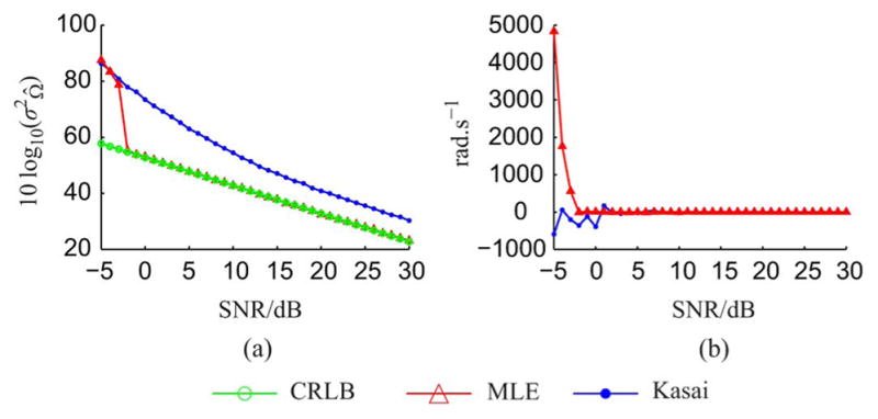
(a) The sample variance of estimates (simulated) compared with the CRLB, for N = 32, T = 0.001 s. The y-axis is the estimator variance in decibels. The variance of the MLE can be seen to rapidly approach the bound even at low SNRs. The Kasai estimator is more than 7 dB worse than the MLE, even at high SNRs. (b) Estimator bias in radians per second with SNR. For moderate SNRs, these values are too small to be significant, hence the estimator variance and the MSE can be considered to be the same.
B. Varying Acquisition Rate
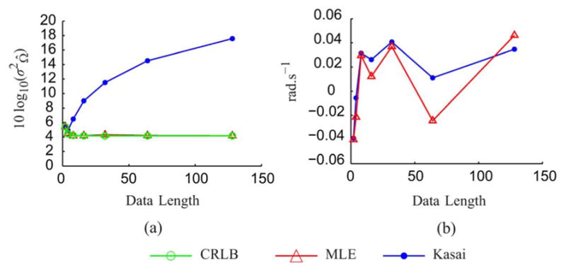
The scaling of estimator performance with acquisition rate is an important consideration, especially as high-speed Doppler OCT imaging in the range of kHz to a few MHz becomes possible. Ordinarily, when the acquisition rate is increased, the number of photons collected from the sample per time step is reduced, and hence SNR scales as Δt = T/N. In some applications it is possible to compensate the increase in acquisition rate with an increase in power on the sample, such that the SNR remains unchanged. Fig. 3 shows that, at an SNR of 36.5 dB, the MLE closely matches the CRLB for data lengths of eight and higher. The performance of the MLE and the CRLB improves with data length. The Kasai estimator variance, on the other hand, either remains roughly constant or increases as the data length is increased. Note that, theoretically, one can make a frequency estimate with either the Kasai estimator or MLE with as few as two data points. However, the Nyquist sampling theorem still applies. In our simulations, a data length of two corresponds to an acquisition rate of 1 kHz and a Nyquist frequency of 500 Hz.
Fig. 3.
(a) Variance of Kasai and ML estimators (simulated) against data length (varying acquisition rate), for T = 0.002 s at a constant SNR of 36.5 dB. In practice, holding the SNR constant would require increasing the detected photon rate (power) with increasing acquisition rate. The acquisition rates used were 20, 21, …, 26 kHz. The Kasai estimator performance does not improve significantly with data length. The MLE performance improves with data length and closely matches the CRLB. (b) Bias estimates for Kasai estimator and MLE suggest that at 36.5 dB SNR, both are unbiased.
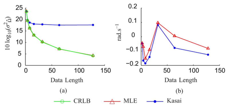
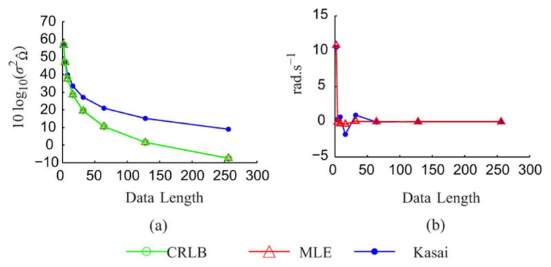
In other applications, such as retinal imaging, the total power on the sample is limited; thus the SNR will be reduced as the acquisition rate is increased. In such cases, the total number of photons collected from the sample remains the same even if the acquisition rate is increased. When we incorporate this type of noise scaling, as shown in Fig. 4, we see that there is little or no improvement of estimator performance with data length for the CRLB and the MLE. This behavior is intuitive, as the total number of photons detected during the acquisition time, T, remains the same, hence the estimator performance is not expected to improve appreciably. Furthermore, this behavior agrees with the limit derived in (21). The Kasai estimator, on the other hand, increases its variance and becomes more inefficient as the data length (acquisition rate) is increased.
Fig. 4.
(a) Variance of Kasai and ML estimators (simulated) with shot noise SNR scaling for T = 0.002 s against data length (varying acquisition rate). This corresponds to maintaining a constant detected photon rate (power) with increasing acquisition rate. The SNRs for N = 2, 4, …, 128 were 54.6, 51.6, 48.6, 45.6, 42.6, 39.5, and 36.5, respectively, approximating the experimental values encountered in Fig. 6 and Table II. The acquisition rates were 20,21, …, 26 kHz. The SNR scales as T/N, hence the CRLB is constant with data length, as shown in (21). The Kasai estimator performance deteriorates with increasing sampling rate. (b) Bias estimates for Kasai estimator and MLE suggest that, both are unbiased.
C. Varying Acquisition Time
Fig. 5 shows that the performance of the estimators improves with increasing acquisition time, as predicted by (19). In particular for N sufficiently large, the scaling of the MLE variance as 1/T3 predicted from (21) is demonstrated. The MLE performance improves at a greater rate than the Kasai estimator with increasing acquisition times.
Fig. 5.
(a) Variance of Kasai and ML estimators against data length (varying acquisition time), for a constant acquisition rate of 47 kHz at an SNR of 36.5 dB. Compare these simulated data with Fig. 7. As the acquisition time is increased, both estimator variances and the CRLB are reduced. The MLE performance closely matches that of the CRLB. (b) Bias estimates for Kasai estimator and MLE suggest that both are unbiased.
VI. Experimental Verification
A. System Description
A 1310 nm spectral/Fourier domain OCT microscope was used for the imaging of a flow phantom. The light source consisted of two superluminescent diodes combined by using a 50/50 fiber coupler to yield a spectral bandwidth of 170 nm. The axial (depth) resolution was 3.6 μm, full-width at half-maximum, and the transverse resolution was 7.2 μm (full-width at half-maximum), and the highest imaging speed was 47 000 axial scans per second, achieved by an InGaAs line scan camera (Goodrich–Sensors Unlimited, Inc.). The camera sensitivity was typically set to “medium” to obtain the widest dynamic range. The high sensitivity setting typically resulted in a signal saturating the camera pixels. A 5× objective, Mitsutoyu, was used and either the coverglass or the center of tubing was placed in focus.
B. Stationary Cover-Glass
We tested the variance of the Kasai and ML estimators by using our OCT system to image a slightly defocused region of the top of a cover-glass slip. The estimated SNR increased with acquisition rate (see Table II). We took an M-scan of a single location. As the cover-glass was stationary, there should be a zero Doppler shift. Hence the bias of the Doppler frequency estimators can be estimated as the difference from zero. To normalize the signal, we divided the signal value of the upper layer of the cover glass by that of the lower layer. We tested the data for normality by running a one sample two-sided Kolmogorov-Smirnov test on the real part of the data. We tested 51 200 data points for four acquisition rates, using the test statistic (x − x̄)/σ. The p-values obtained were 0.0024, 0.9219, 0.0473, and 3 × 10⁻⁷ for 17.3 μs, 34.6 μs, 69.2 μs, and 138.4 μs sampling times, respectively. We do not reject the null hypothesis that the noise is normal for 34.6 μs. However, for the other acquisition rates, we would reject the null hypothesis at a 5% significance level. Still, this may be within the 10% level of contamination typically accepted for an AWGN model [20], [21]. We confirmed that the noise was Gaussian using quartile–quartile plots. For the rates where the null hypothesis was rejected, distribution had slightly fatter tails than in a Gaussian distribution.
Table II.
SNRs at Various Acquisition Rates for Cover-Glass Experiment. We Took the Ratio of the Average of the Absolute Value of the Measured Signal, |sn|2, and the Variance of the Signal, Var (sn), as an Estimate of the SNR. As There is Some Periodicity in the Signal, the Estimate Will be Data Length Dependent. Each Acquisition Cycle has an Inactive Period of Around 4.0 μs
| Integration time/μs | Acquisition Rate/kHz | Data length | SNR/dB |
|---|---|---|---|
| 553.6 | 1.8 | 4 | 53.8 |
| 276.8 | 3.6 | 8 | 53.0 |
| 138.4 | 7.0 | 16 | 49.2 |
| 69.2 | 13.7 | 32 | 44.5 |
| 34.6 | 25.9 | 64 | 40.0 |
| 17.3 | 47.0 | 128 | 36.5 |
Fig. 6(a) shows that for a constant acquisition time of approximately 0.0025 s, the performance of the MLE follows that of the CRLB. The performance of the Kasai estimator was worse, and deteriorated with higher acquisition rates. The experimental results are consistent with simulation, as shown in Fig. 4(a). The CRLB remains roughly constant with acquisition rate, as predicted by theory and simulation. The estimators performed as predicted by simulation and theory, though they appear to have a slightly worse performance than Fig. 4(a), as a slightly longer acquisition time was used. A 3 dB estimator improvement can be attributed to a 25% increase in acquisition time, due to the relationship, CRLB ∝1/T3(21).
Fig. 6.
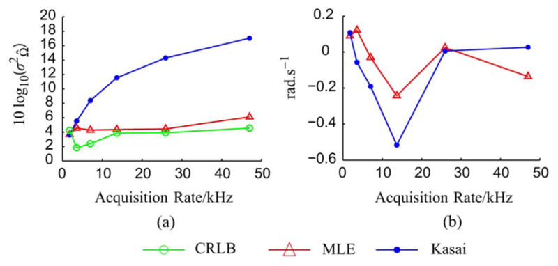
(a) Plot of experimentally determined estimator performance against acquisition rate from a fixed M-scan of a nonmoving cover-glass, estimated from 100 samples, with T ≈ 0.0025 s. The SNRs (see Table II) were estimated from data and used to determine the CRLB. The experimentally measured SNR was 36.5 dB for an acquisition rate of 47 kHz. These results are in agreement with Fig. 4, taking into account a longer acquisition time. (b) The bias estimates are on the order of tenths of rad.s−1, which is negligible and the estimators can be assumed to be unbiased.
However, with increasing acquisition time, the MLE performance deviates from the CRLB, as shown in Fig. 7(a). This is due to the increased effect of other sources of noise such as galvanometer noise and phase instabilities of the acquisition system.
Fig. 7.
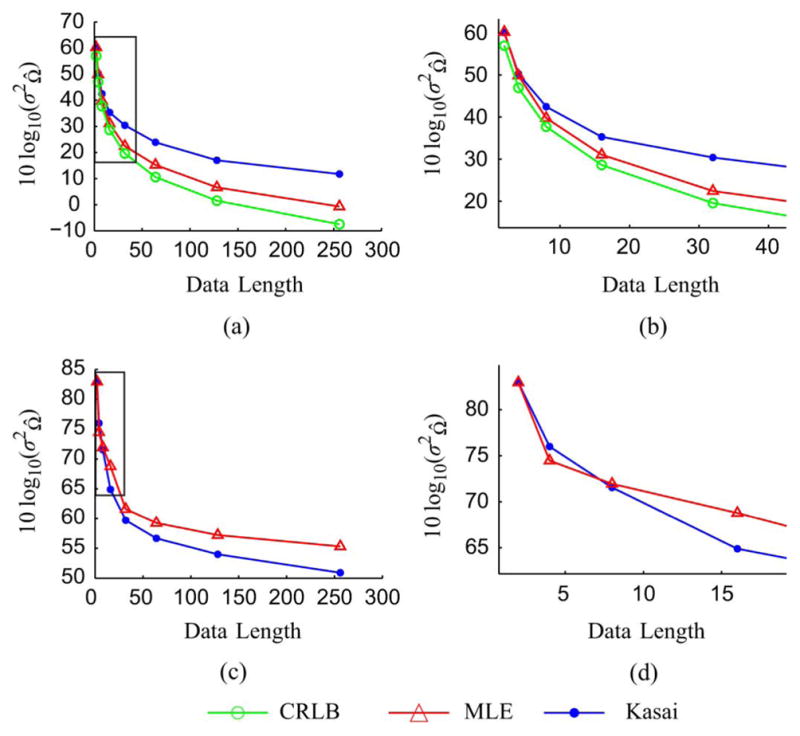
(a), (b) Experimental verification of the Kasai and ML estimator variances against data length (acquisition time), for constant acquisition rate of 47 kHz measured on the surface of a cover-glass. The CRLB was plotted assuming a 36.5 dB SNR. Compare this figure with Fig. 5(a). The MLE slowly diverges from the CRLB as acquisition times increase, contrary to the prediction from simulation, due to other sources of noise. (c), (d) Verification using a 0.1 ml.hr−1 intralipid flow phantom, at about one quarter in from the edge of the tubing. The SNR was approximately 10.0 dB. The MLE performs better than the Kasai estimator for data lengths of up to 8 or acquisition times of up to 0.17 ms. For data lengths longer than this, decorrelation noise becomes significant and the MLE performance becomes worse.
C. Intralipid Flow Phantom
We used Intralipid-10% [32] and a syringe pump with 0.58-mm-diameter tubing. Intralipid globules have an average diameter of 100 nm. The pipe was placed at a 16° incline, so that there was an axial velocity which could be measured by calculating the shift in the position of the peak of the PSD. Fluid flow in a tube has a Poiseuille profile, hence measurements of the Doppler shift were taken at 0.16 mm from the inner edge of the tubing. Fig. 7 shows that for a 0.1 ml.hr−1 flow rate, our MLE performs better than the Kasai estimator for short acquisition times. For data lengths above 8 (acquisition times longer than 0.17 ms) decorrelation noise becomes dominant and the MLE performance becomes worse than the Kasai performance. The effects of decorrelation, are negligible if acquisition time is less than the coherence time of the signal, but increase as acquisition times increase. Other sources of noise, including galvanometer jitter, thermal drift, and other phase instabilities could also contribute to a worse performance, as these effects are also amplified with increasing acquisition time. As the actual value of the Doppler frequency is not known with sufficient precision in the flow phantom experiments, one cannot estimate the bias.
VII. Model Limitations
A. Decorrelation Noise
“Decorrelation noise” [25] is caused by random deviations of the signal. This is primarily due to the entry and exit of different red blood cells (RBCs) into and out of a voxel. The random distribution of RBC position, speed, orientation or shape are also contributing factors. In addition, the translation of the probe beam due to transverse scanning contributes to decorrelation. Decorrelation is typically characterized by a time scale, known as the coherence time, after which the complex amplitude is randomized. The value of the complex OCT signal at any given time would have much less predictive value after the coherence time has passed.
Our results show that good estimation performance can be achieved by the MLE with a simple AWGN model, under restricted conditions that obey the model assumptions. However, for many in vivo applications, decorrelation noise [25] is present, as shown in our flow phantom experiments. This would broaden the peak of the power spectral density (PSD), and lower its height. The MLE derived here, which takes the frequency estimate as the position of the peak of the power spectral density, assumes AWGN and would be suboptimal in the presence of a significant amount of decorrelation noise. For our experimental verification of the MLE, we chose conditions where decorrelation is minimized, such as scanning a stationary glass coverslip or very slow flow. Fig. 8 shows experimental verification of these estimators, at an acquisition time where decorrelation noise begins to become significant. Beyond roughly 0.2 ms, the MLE performance is no longer superior to that of the Kasai estimator. We thus propose that further estimation accuracy under a broader range of conditions may be achieved by incorporating decorrelation noise into the noise model.
Another important limitation of this model, especially for Doppler ultrasound, is the assumption of ergodicity [33]. In reality, blood flow is pulsatile and velocities would have some periodicity. In our phantom experiments, a syringe pump does not produce a constant pressure differential. In this work, however, our acquisition times in both simulation and experiment were in the order of milliseconds, and for normal human heart rates, this time is sufficiently short to estimate an instantaneous velocity. To apply our analysis to the slower acquisition rates of pulse-echo ultrasound would require modifications to the analysis in this paper to account for the pulsatile flow.
B. Performance With Multiplicative Noise
The effects of decorrelation noise can be modelled with multiplicative noise [34]. To achieve this we modified the signal from (6) to include a multiplicative term qn and assumed negligible additive noise
| (24) |
where qn is a correlated complex Gaussian random variable, with each of the real and imaginary parts having variance σ2 = 1/2, hence Var (qn) = 1. The variance was chosen without loss of generality. We predetermined the auto-covariance matrix of qn to be real Toeplitz, with the first row (the auto-covariance function) being the values of a Gaussian profile from the non-negative domain. Its 1/e full-width is determined by the coherence time of the signal, and was set to be 4Δt = 0.125 ms for these simulations. The continuous parameter m is used to vary the relative amount of multiplicative noise compared with the static reflectivity, or noiseless signal.
Fig. 9 shows that the AWGN MLE performance deteriorates more rapidly than the Kasai estimator with an increasing proportion of multiplicative noise. This suggests the Kasai estimator’s greater robustness against decorrelation noise. In the signal dominant regime, the AWGN MLE performs better. In the multiplicative decorrelation noise dominant regime, the Kasai estimator performs better.
Fig. 9.
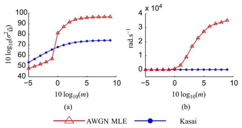
(a) The sample variance of estimates for varying degrees of multiplicative noise with no additive noise for, N = 32, T = 0.001 s. The x-axis shows the ratio of multiplicative noise components to signal components in decibels. At roughly −0.5 dB the estimators have equal performance. (b) Estimator bias in radians per second with SNR.
VIII. Conclusion
Estimator efficiency and performance scaling with data acquisition rate are important properties to consider as Doppler OCT imaging speeds continue to improve. Using a simple additive white Gaussian noise model, we have shown that MLEs are preferable to the more computationally simple Kasai estimator. We confirmed that the variance of the commonly-used Kasai estimator increases with increasing acquisition rate, and the Kasai estimator becomes less efficient. The performance of the Kasai estimator deteriorates with higher acquisition rates while the detected photon rate (power) is kept constant, and this makes it unsuitable as a Doppler frequency estimator as OCT acquisition speeds increase. This is nonintuitive and paradoxical behavior, since increasing the sampling rate (while keeping the total number of detected photons the same) should provide more information about parameters to be estimated.
By contrast, we have shown that the CRLB for estimator variance, for a sufficiently high number of samples, is proportional to 1/T3(21), and is independent of the sampling rate. As the CRLB gives us the theoretical best performance, this suggests that there are better alternatives to the Kasai estimator. Since the MLE variance approaches the CRLB asymptotically, the MLE also asymptotically possesses this desirable and intuitive property. Therefore, our results suggest that the MLE may be the estimator of choice for high Doppler OCT imaging rates. Contrary to the results of [12], we have shown that the MLE asymptotically outperforms the Kasai estimator under assumptions of additive white Gaussian noise.
Several caveats and limitations must also be discussed. First, the desirable asymptotic properties of the MLE may not hold for smaller numbers of samples. Second, decorrelation noise reduces estimator performance, especially at longer acquisition times. However, we anticipate that it should be possible to define a more general MLE that incorporates the effects of decorrelation with an appropriate statistical model [26]. Third, as performance of parametric estimators can be sensitive to deviations from the assumed noise model, there is room for further development of robust [20] estimation techniques. Finally, one may also formulate efficient linear estimators that achieve MLE-like performance [35], [36].
Acknowledgments
This work was supported in part by the University Research Committee of the University of Hong Kong under Project 10401797, in part by in part by the National Institutes of Health (R00NS067050, EB001954 R01), in part by the American Heart Association (11IRG5440002), and in part by the Glaucoma Research Foundation Catalyst for a Cure.
The authors would like to thank Dr. M. A. Franceschini for permission to use the OCT system.
Footnotes
Color versions of one or more of the figures in this paper are available online at http://ieeexplore.ieee.org.
Contributor Information
Aaron C. Chan, Email: cwachan@eee.hku.hk, Department of Electrical and Electronic Engineering, University of Hong Kong, Pokfulam, Hong Kong.
Edmund Y. Lam, Email: elam@eee.hku.hk, Department of Electrical and Electronic Engineering, University of Hong Kong, Pokfulam, Hong Kong.
Vivek J. Srinivasan, Email: vjsriniv@ucdavis.edu, vjsriniv@nmr.mgh.harvard.edu, Biomedical Engineering Department, University of California–Davis, Davis, CA 95616 USA, and also with MGH/MIT/HMS Athinoula A. Martinos Center for Biomedical Imaging, Massachusetts General Hospital/Harvard Medical School, Charlestown, MA 02129 USA
References
- 1.Izatt JA, Kulkarni MD, Yazdanfar S, Barton JK, Welch AJ. In vivo bidirectional color Doppler flow imaging of picoliter blood volumes using optical coherence tomography. Opt Lett. 1997 Sep;22(18):1439–1441. doi: 10.1364/ol.22.001439. [DOI] [PubMed] [Google Scholar]
- 2.Chen Z, Milner TE, Dave D, Nelson JS. Optical Doppler tomographic imaging of fluid flow velocity in highly scattering media. Opt Lett. 1997 Jan;22(1):64–66. doi: 10.1364/ol.22.000064. [DOI] [PubMed] [Google Scholar]
- 3.Srinivasan VJ, Sakadzic S, Gorczynska I, Ruvinskaya S, Wu W, Fujimoto JG, Boas DA. Quantitative cerebral blood flow with optical coherence tomography. Opt Exp. 2010 Feb;18(3):2477–2494. doi: 10.1364/OE.18.002477. [DOI] [PMC free article] [PubMed] [Google Scholar]
- 4.Nezam SMM, Joo C, Tearney GJ, de Boer JF. Application of maximum likelihood estimator in nano-scale optical path length measurement using spectral-domain optical coherence phase microscopy. Opt Exp. 2008 Oct;16(22):17186–17195. doi: 10.1364/oe.16.17186. [DOI] [PMC free article] [PubMed] [Google Scholar]
- 5.Szkulmowski M, Szkulmowska A, Bajraszewski T, Kowalczyk A, Wojtkowski M. Flow velocity estimation using joint spectral and time domain optical coherence tomography. Opt Exp. 2008 Apr;16(9):6008–6025. doi: 10.1364/oe.16.006008. [DOI] [PubMed] [Google Scholar]
- 6.Szkulmowska A, Szkulmowski M, Kowalczyk A, Wojtkowski M. Phase-resolved Doppler optical coherence tomography-limitations and improvements. Opt Lett. 2008 Jul;33(13):1425–1427. doi: 10.1364/ol.33.001425. [DOI] [PubMed] [Google Scholar]
- 7.Doisy Y. Theoretical accuracy of Doppler navigation sonars and acoustic Doppler current profilers. IEEE J Ocean Eng. 2004 Apr;29(2):430–441. [Google Scholar]
- 8.Kasai C, Namekawa K, Koyano A, Omoto R. Real-time two-dimensional blood flow imaging using an autocorrelation technique. IEEE Trans Sonics Ultrason. 1985 May;32(3):458–464. [Google Scholar]
- 9.Yeh CK, Ferrara K, Kruse D. High-resolution functional vascular assessment with ultrasound. IEEE Trans Med Imag. 2004 Oct;23(10):1263–1275. doi: 10.1109/TMI.2004.834614. [DOI] [PubMed] [Google Scholar]
- 10.Arigovindan M, Suhling M, Jansen C, Hunziker P, Unser M. Full motion and flow field recovery from echo Doppler data. IEEE Trans Med Imag. 2007 Jan;26(1):31–45. doi: 10.1109/TMI.2006.884201. [DOI] [PubMed] [Google Scholar]
- 11.Pinter S, Lacefield J. Objective selection of high-frequency power Doppler wall filter cutoff velocity for regions of interest containing multiple small vessels. IEEE Trans Med Imag. 2010 May;29(5):1124–1139. doi: 10.1109/TMI.2010.2041246. [DOI] [PubMed] [Google Scholar]
- 12.Yazdanfar S, Yang C, Sarunic M, Izatt J. Frequency estimation precision in Doppler optical coherence tomography using the Cramer-Rao lower bound. Opt Exp. 2005 Jan;13(2):410–416. doi: 10.1364/opex.13.000410. [DOI] [PubMed] [Google Scholar]
- 13.Loupas T, Powers J, Gill R. An axial velocity estimator for ultrasound blood flow imagingbased on a full evaluation of the Doppler equation by means of a two-dimensional autocorrelation approach. IEEE Trans Ultrason Ferroelectr Freq Control. 1995 Jul;42(4):672–688. [Google Scholar]
- 14.Hoeks APG, Peeters HHPM, Ruissen CJ, Reneman RS. A novel frequency estimator for sampled Doppler signals. IEEE Trans Biomed Eng. 1984 Feb;31(2):212–220. doi: 10.1109/TBME.1984.325331. [DOI] [PubMed] [Google Scholar]
- 15.Tschirren J, Lauer RM, Sonka M. Automated analysis of Doppler ultrasound velocity flow diagrams. IEEE Trans Med Imag. 2001 Dec;20(12):1422–1425. doi: 10.1109/42.974936. [DOI] [PubMed] [Google Scholar]
- 16.Hardesty R. Performance of a discrete spectral peak frequency estimator for Doppler wind velocity measurements. IEEE Trans Geosci Remote Sens. 1986 Sep;24(5):777–783. [Google Scholar]
- 17.Lehmann EL, Casella G. Theory of Point Estimation. 2. New York: Springer-Verlag; 1998. [Google Scholar]
- 18.Schmoll T, Kolbitsch C, Leitgeb RA. Ultra-high-speed volumetric tomography of human retinal blood flow. Opt Exp. 2009 Mar;17(5):4166–4176. doi: 10.1364/oe.17.004166. [DOI] [PubMed] [Google Scholar]
- 19.Wojtkowski M, Srinivasan V, Ko T, Fujimoto J, Kowalczyk A, Duker J. Ultrahigh-resolutionhigh-speedFourier domain optical coherence tomography and methods for dispersion compensation. Opt Exp. 2004 May;12(11):2404–2422. doi: 10.1364/opex.12.002404. [DOI] [PubMed] [Google Scholar]
- 20.Hampel FR. Robust Statistics: The Approach Based on Influence Functions. 18. New York: Wiley; 1986. [Google Scholar]
- 21.Huber PJ. Robust Statistical Procedures. 2. Philadelphia: SIAM; 1996. [Google Scholar]
- 22.Stark H, Woods JW. Probability and Random Processes with Applications to Signal Processing. 3. New York: Prentice Hall; 2001. [Google Scholar]
- 23.Papoulis A, Pillai SU. Probability, Random Variables and Stochastic Processes. 4. New York: McGraw-Hill; 2001. [Google Scholar]
- 24.Kay SM. Fundamentals of Statistical Signal Processing: Estimation Theory. Vol. 1 New York: Prentice Hall; 1993. [Google Scholar]
- 25.Vakoc B, Tearney G, Bouma B. Statistical properties of phase-decorrelation in phase-resolved Doppler optical coherence tomography. IEEE Trans Med Imag. 2009 Jun;28(6):814–821. doi: 10.1109/TMI.2009.2012891. [DOI] [PMC free article] [PubMed] [Google Scholar]
- 26.Chan AC, Lam EY, Srinivasan VJ. Doppler frequency estimators under additive and multiplicative noise. Proc SPIE. 2013 Feb;8571 [Google Scholar]
- 27.Forsythe GE, Malcolm MA, Moler CB. Computer Methods for Mathematical Computations. New York: Prentice-Hall; 1976. [Google Scholar]
- 28.Ahn YB, Park SB. Estimation of mean frequency and variance of ultrasonic Doppler signal by using second-order autoregressive model. IEEE Trans Ultrason Ferroelectr Freq Control. 1991 May;38(3):172–182. doi: 10.1109/58.79600. [DOI] [PubMed] [Google Scholar]
- 29.Herment A, Demoment G, Dumee P. Improved estimation of low velocities in color Doppler imaging by adapting the mean frequency estimator to the clutter rejection filter. IEEE Trans Biomed Eng. 1996 Sep;43(9):919–927. doi: 10.1109/10.532126. [DOI] [PubMed] [Google Scholar]
- 30.Cloutier G, Chen D, Durand LG. A new clutter rejection algorithm for Doppler ultrasound. IEEE Trans Med Imag. 2003 Apr;22(4):530–538. doi: 10.1109/TMI.2003.809059. [DOI] [PubMed] [Google Scholar]
- 31.Oppenheim AV, Schafer RW, Buck JR. Discrete-Time Signal Processing. 2. New York: Prentice Hall; 1989. [Google Scholar]
- 32.Staveren Hv, Moes C, Marle Jv, Prahl S, Gemert Mv. Light-scattering in intralipid-10-Percent in the wavelength range of 400–1100 nm. Appl Opt. 1991 Nov;30(31):4507–4514. doi: 10.1364/AO.30.004507. [DOI] [PubMed] [Google Scholar]
- 33.Goodman JW. Statistical Optics. New York: Wiley; 1985. [Google Scholar]
- 34.Chan AC, Lam EY, Srinivasan VJ. Optimal Doppler frequency estimators for ultrasound and optical coherence tomography. IEEE Biomed Circuits Syst Conf. 2012 Nov;:264–267. [Google Scholar]
- 35.Tufts D, Kumaresan R. Estimation of frequencies of multiple sinusoidsMaking linear prediction perform like maximum likelihood. Proc IEEE. 1982 Sep;70(9):975–989. [Google Scholar]
- 36.Wang H, Kay S. Maximum likelihood angle-Doppler estimator using importance sampling. IEEE Trans Aerosp Electron Syst. 2010 Apr;46(2):610–622. [Google Scholar]