

Abstract
This paper examines the relationship between neighborhood disorder and anxiety symptoms. It draws on data from the Monitoring Mt. Laurel Study, a new survey-based study that enables us to compare residents living in an affordable housing project in a middle-class New Jersey suburb to a comparable group of non-residents. Using these new data, we test the hypothesis that living in an affordable housing project in a middle class suburb reduces a poor person’s exposure to disorder and violence compared to what they would have experienced in the absence of access to such housing, and that this lesser exposure to disorder and violence yields improvements in anxiety that can be attributed to residents’ reduced stress burden. We find that residents of the project are less likely to be exposed to disorder and violence and have lower stress levels and slightly fewer anxiety symptoms. Differences in exposure to disorder explain differences in stress burden, and, hence, anxiety symptoms between the two groups.
Keywords: Neighborhood effects, Mental health, Anxiety, Poverty, Disorder, Stress
The publication of William Julius Wilson’s landmark book, The Truly Disadvantaged (1987), repositioned neighborhood ecology as an important factor in explaining individual-level disparities. That economic, social, and even physical well-being were products not only of individual- and family-level attributes but also neighborhood processes was an idea that was consistent with the Chicago School’s early emphasis on ecology and community context, but had lost traction in the 1970 s and 1980 s as sociologists shifted their attention toward using large-scale surveys to study individual-level outcomes (Massey, 2001; Clampet-Lundquist and Massey, 2008).
Wilson made a convincing case for the concentration of poverty and its importance as a determinant of human behavior and his work acted as a stimulus to further empirical study of the processes governing these relationships. Much of the early research on “neighborhood effects” simply merged survey and census data to look for relationships between neighborhood poverty and individual-level outcomes. This work was important for establishing that poverty rates vary dramatically across neighborhoods; that there is considerable variation in violence, poor health, joblessness, and other undesirable conditions across neighborhoods; and that there is a statistical correlation between neighborhood disadvantage and various individual-level outcomes (Sampson et al., 2002; Sampson, 2003).
The last 20 years have witnessed improvements in both the theorization and measurement of the social processes underlying the relationship between neighborhood conditions and individual well-being (Sampson et al., 1997, 1999; Raudenbush and Sampson, 1999), and in the types of statistical models applied to the study of these processes (see, e.g., Garner and Raudenbush, 1991; Bryk and Raudenbush, 1992; Harding, 2003). Yet, while these observational studies were able to demonstrate strong statistical associations between neighborhood ecology and a range of economic, social, and health outcomes, they told us little about whether neighborhood conditions have any causal impact on behavior and well-being or whether individuals with certain traits simply select into certain neighborhoods (Jencks and Mayer, 1990; Tienda, 1991).
The application of experimental and quasi-experimental research designs to the study of neighborhood effects has enabled researchers to make some progress on this issue. The Gautreaux studies followed poor Chicago residents who were given vouchers to relocate out of segregated communities and offered some evidence that participants who moved into low-minority, suburban neighborhoods experienced higher employment, while their children showed improved educational and employment outcomes relative to those who stayed in Chicago (Rubinowitz and Rosenbaum, 2000; Popkin et al., 1993), though there is some evidence that these gains did not persist in the long run (DeLuca et al., 2010). Yet the Gautreaux project was not a true experiment; residents were not randomly assigned to receive vouchers; so the possibility that these findings were spurious remained. In response, the U.S. Department of Housing and Urban Development funded a demonstration project to move residents of public housing projects in five cities into non-poor neighborhoods, but this time researchers employed an experimental research design to correct for selection bias. The Moving to Opportunity (MTO) project randomly assigned residents to one of the three groups: a treatment group that received vouchers to move to a low-poverty neighborhood, a group that received Section 8 vouchers but could move wherever they desired, and a control group that did not receive vouchers. The study boasted a pre-post design that enabled researchers to collect data prior to the administration of vouchers and then at several follow-up points, and was seen as the first chance to apply the rigors of experimental research to Wilson’s hypothesis.
Results from the MTO program suggest it was successful in moving people out of poor neighborhoods and that living in non-poor neighborhoods had positive effects on adult mental health, but that living in non-poor neighborhoods had little positive effect on participants’ economic and physical well-being (Kling et al., 2007; Orr et al., 2003). The bulk of this research seems to suggest that neighborhoods matter for some outcomes, but not all, and that the benefits accrue more to females than males (Sampson, 2008).
Some argue that this dearth of promising findings, particularly regarding adults’ economic self-sufficiency, can be attributed to the design and implementation of the MTO program (for a fuller review of these issues, see Clampet-Lundquist and Massey, 2008). For instance, some participants assigned to the treatment group opted not to use their vouchers to move out of their neighborhoods, introducing selection bias into the study. In addition, although the MTO data may provide estimates of the effects of moving to a non-poor neighborhood after receipt of a housing voucher, they are not as useful for measuring the effect of living in a low-poverty neighborhood. If participants moved into non-poor neighborhoods but only stayed for a short period of time, and we do not account for this in our models, then results may be biased by selective outmigration (Clampet-Lundquist and Massey, 2008).
The present paper examines the relationship between neighborhood disorder and individual-level anxiety outcomes. It draws on data from the Monitoring Mt. Laurel Study, a new survey-based study that enables us to compare residents living in an affordable housing project in a middle-class New Jersey suburb to a comparable group of non-residents who applied to live in the project but were not accepted in the project or were still on the waiting list at the time the survey was administered, thus holding constant self-selection into the pool of people wishing to move into affordable suburban housing. The quasi-experimental design of the Mt. Laurel Study is well-suited for the study of neighborhood effects and overcomes some of the limitations of the MTO experiment. At the time the data were collected, for example, most residents had lived in the project for several years, some for as long as 10 years. This means that enough time had elapsed to allow hypothesized cumulative effects to emerge, thus enabling us to disentangle neighborhood effects from the effects of moving. We also had access to residents’ and non-residents’ initial applications to enter the project and we drew on these applications to estimate scores to capture the likelihood of moving from the applicant list into the project. We use these propensity scores to match residents to non-residents on the measures that influenced entry into the project.
Using these new data, we test the hypothesis that living in an affordable housing project in a middle class suburb reduces a poor person’s exposure to disorder and violence compared to what they would have experienced in the absence of access to such housing, and that this lesser exposure to disorder and violence yields improvements in mental health that can be attributed to residents’ reduced stress burden. We begin by reviewing theory and research on the relationship between neighborhood context and health status before offering a brief history of the Mt. Laurel housing project and its present configuration. We then outline our data and measures and subject them to a series of multivariate analyses, and determine the direct and indirect effects of living in a suburban housing project on anxiety symptoms. In a preview of our findings, we find very small differences between residents and non-residents of the housing project in reported anxiety symptoms. We show that these differences can be explained almost entirely by differences in exposure to neighborhood disorder and, hence, stressful life events. We conclude with a summary of our findings and their implications for affordable housing policy.
1. Neighborhood conditions and individual mental health
We hypothesize that living in a housing project in a middle-class suburb reduces residents’ exposure to social disorder, crime and violence, which in turn decreases their likelihood of experiencing stressful life events and consequently lowers their anxiety symptoms relative to what they might experience in a poorer neighborhood. We present this hypothesized causal sequence in Fig. 1.
Fig. 1.
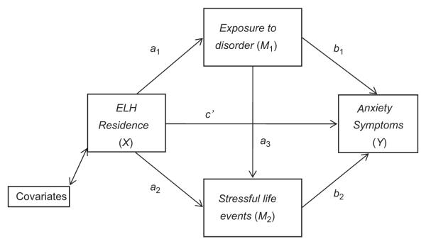
Path diagram showing the direct effect and causal paths linking ELH residence to anxiety symptoms.
Why do neighborhood economic conditions affect one’s exposure to disorder? Poor neighborhoods lack the social interactional processes that are crucial for community social control and thus are at a higher risk for social disorganization. Robert Sampson and colleagues find that poor, unstable communities have lower rates of “collective efficacy,” or shared expectations that neighbors will intervene to control their neighborhood, and that lower rates of collective efficacy in turn increase the level of violence in the community (Sampson et al., 1997, 1999). As a result, individuals living in poor communities are more likely to witness violence and crime than their counterparts in non-poor communities. Members of the MTO treatment group reported, for example, that they felt safer in their neighborhoods and observed less crime and disorder than members of the control group (Katz et al., 2001).
Repeated exposure to disorder and violence may in turn increase an individual’s likelihood of experiencing stressful life events. First, physical proximity to violence, drug use, and gang presence undoubtedly increase one’s chances of being victimized in the form of burglary, robbery, or physical assault. Living in close proximity to violence and disorder also impacts the composition of one’s social networks, such that residents have increased contact with people involved in illegal activity and less contact with positive role models, increasing their likelihood of dropping out of school, having an unplanned pregnancy, and becoming involved in illicit activity (Harding, 2003; Kling et al., 2005; Lindberg and Orr, 2011). In short, residents of poor neighborhoods are embedded in a well-known “tangle of pathology” (Clark, 1965) that affects their decision-making and bears on the number of stressful events they experience over time.
Moreover, living in an environment of chaos and disorder places the body in a state of heightened physiological arousal, which ultimately leads to heightened physiological stress. Prolonged exposure to violence and disorder repeatedly initiates the fight or flight response, stimulating the release of adrenaline, cortisol, and other stress hormones to raise allostatic load, or the degree to which an organism is over-exposed to physiological responses that are adaptive when experienced infrequently and sporadically but destructive when triggered repeatedly over an extended period of time. Excessive adrenaline and cortisol in the bloodstream over time heightens one’s aggressiveness and impulsiveness and prompts risky behavior and poor decision-making (McEwan, 1992; McEwan and Lasley, 2002; Massey, 2004). A person with these traits may in turn be more likely to self-medicate with drugs and alcohol, which can further heighten allostatic load and cause physical damage to the body (McEwan and Lasley, 2002; Ross and Mirowsky, 2001). To summarize, neighborhood poverty has a known impact on residents’ exposure to violent activity and disorder whereas prolonged exposure to such stressors is hypothesized to increase allostatic load to undermine psychological well-being.
Observational evidence indeed suggests an empirical association between neighborhood poverty and mental health status.Mair et al. (2008) review of observational studies testing the link between neighborhood characteristics and depressive symptoms provides strong cross-sectional evidence that neighborhood conditions are related to mental health. Galea et al. (2006), for instance, use data from a prospective cohort study to show that adults residing in poorer New York City neighborhoods were significantly more likely to develop depressive symptoms over an 18 month period than adults in high-SES neighborhoods.
The literature further suggests that exposure to neighborhood disorder and stress plays a salient role in mediating the neighborhood–mental health relationship. Aneshensel and Sucoff (1996) show that adolescents in poor neighborhoods in Los Angeles are more likely to perceive their neighborhoods as being dangerous, which in turn heightens symptoms of depression, anxiety and other mental health conditions. Hill et al.’s (2005) work offers evidence that neighborhood disadvantage increases psychological stress, which in turn has negative consequences for individual physical health, echoing Ross and Mirowsky’s (2001) earlier finding that the negative relationship between neighborhood poverty and health status is mediated entirely by exposure to neighborhood disorder and the fear associated with witnessing stressful events (see also Boardman, 2004).
There is also some experimental evidence linking neighborhood conditions to individual health, as adults in the experimental MTO group reported better mental health than the control group (Kling et al., 2007; Katz et al., 2001). Researchers were unable to test why neighborhood conditions influenced mental health in this way, though qualitative interviews with MTO participants indicated that stress reduction was likely the primary reason (Kling et al., 2007; see also Popkin et al., 2002). In short, empirical evidence suggests a relationship between neighborhood disorder and self-reported physical and mental health; this same literature shows that disorder and stress are potentially important as mediators of this relationship. Still, there is little work testing these mediating effects in an experimental or quasi-experimental context.
2. The Mt. Laurel case
Mt. Laurel Township is located about 8 miles east of Camden, New Jersey, a severely depressed former manufacturing center that lies just across the Delaware River from Philadelphia. Until the Second World War Mt. Laurel was a small farming community, but afterward it grew into a Philadelphia suburb of around 40,000 residents, with extensive retail and commercial development and thousands of jobs attracted there because of its location at the intersection of major highways. In many ways, it represents a classic suburban community. According to data from the 2000 Census, it is predominantly white (88% of the population) and composed mostly of homeowners (84% of households) living in single family homes (72% of all housing units). A significant proportion of residents live in age-restricted (55+) condominium or townhouse developments.
In 1971 the NAACP filed suit against the Township of Mount Laurel, New Jersey, on behalf of Ethel R. Lawrence and other low income plaintiffs. The suit challenged the township’s restrictive zoning regulations, which effectively prevented the construction of affordable housing within the community, and thus excluded poor families from residence. After a prolonged legal battle, the state Supreme Court in 1975 found for the plaintiffs and articulated what has since come to be known as “the Mount Laurel Doctrine” that municipalities throughout New Jersey have an affirmative obligation to meet their “fair share” of the regional demand for low income housing (Kirp et al., 1995).
The favorable court decision (commonly known as Mt. Laurel I) did not immediately lead to construction, however, as the township fought over what its “fair share” of low income units might be. In 1983 the court reaffirmed its earlier ruling in another decision (known as Mt. Laurel II) and ordered the township to permit the project to move forward (Haar, 1996). Fair Share Housing Development, Inc., a nonprofit developer of affordable housing in South Jersey, began planning a development that came to be known as the Ethel Lawrence Homes.
Plans submitted to township authorities were subject to a long series of acrimonious hearings and public challenges, however, and it was not until April of 1997 that the Township Planning Board finally granted its approval, but not before a series of stormy public hearings attended by more than 500 angry citizens (Smothers 1997a, 1997b, 1997c). The Ethel R. Lawrence Homes were finally built on a 62 acre field and wooded site, adjacent to luxury, market-rate single family detached housing and a retirement community. The development opened in two phases, with 100 initial units in late 2000 and 40 other units early in 2004. It consists of one-, two-, and three-bedroom two-story townhouses that are 100% affordable to lower income households, defined as those with incomes under 80% of the regional median income, who pay no more than 30% of their incomes for rent and utilities. These criteria yield a remarkably broad range of “affordability,” with units going to households with incomes that range from 10% to 80% of the median income, roughly $6200 to $49,500 per year.
In 2000, Fair Share Housing Development began an affirmative marketing program in newspapers and local media, followed by three days during which applications were distributed to all who sought them. The applications were reviewed in the order in which they were returned within each category and evaluated with respect to several selection criteria, including third party verification of income, a five-year history of residence, and a search of public records for criminal, bankruptcy, or landlord judgments. Those who met the entry criteria were interviewed separately to review the information in the file and, upon agreement to the terms of the lease, were offered a spot in the housing complex. Fair Share repeated the application process in 2003, 2006, 2007, and 2010 in order to refresh the waiting list.
3. Methodology
We hypothesize that residing in the Ethel Lawrence Homes (ELH) reduces residents’ exposure to neighborhood disorder, which reduces stressful experiences, which, in turn, reduces their anxiety symptoms. We draw on data from a survey of current and former residents of the Ethel Lawrence Homes and a comparison sample of individuals who applied but, for one reason or another, remained on the waiting list at the time of the survey or had not been accepted into the project. We sought to interview everyone who currently reside in ELH and all former ELH residents for whom we could find a valid address. We also interviewed a sample of applicants who had not yet been accepted or had been rejected for whom we could find a recent address. The survey staff sent letters explaining the study and requesting participation to all potential respondents and then a staff of trained field interviewers followed up with phone calls or, if a phone number could not be identified, home visits. Interviewers administered an in-person, 60-min questionnaire to all willing participants, either in participants’ homes or at a neutral site of their choosing. The interviews were conducted between November 19, 2009, and March 3, 2010.
This method yielded a final sample of 116 residents and 108 non-residents. Of the 116 residents, five were former residents who had moved out of the project by the time of the survey. Not surprisingly, compliance was much higher among residents than non-residents—79% of current and former residents contacted who participated in the survey, compared to 30.3% of non-residents. Table A1 in Appendix A gives the breakdown of the reasons for non-compliance for each group. By far the most important reason for non-response among non-residents was the simple inability to find the respondent (45% of cases), in most cases because they had moved from the address listed on their application form. Among those non-residents who were located, the non-response rate was 55%.
Given that some members of our sample were selected to live in the housing project, while others were not (or have yet to be), it remains a possibility that the two groups differ on unmeasured characteristics that may bear on the outcomes of interest. To control for this, we estimated a model predicting, for each participant in the study, the likelihood, or propensity, of being accepted into the Ethel Lawrence Homes and then use the resulting propensity scores to create matched samples of residents and nonresidents for our final models.1 The propensity models were estimated using data from participants’ initial applications to the Ethel Lawrence Homes, which were archived at Fair Share Housing Development, located on-site at the Homes. The propensity scores are a function of those variables found in the application files; so it remains a possibility that selection into the Homes was affected by unmeasured characteristics that were omitted from the files. Nevertheless, we were able to create a database that included a broad range of relevant data on householder characteristics, including age, household size and composition, relationship status, sex, income, and location and type of residence. In addition to these variables, the applications also included several variables that helped us measure their purported reasons for wanting to move, their actual motivation to enter the project, as indicated by their number on the first-come-first-served waiting list, and their access to family resources, as indicated by whether they were currently living with a family member. Descriptions of these variables and the results from the propensity score analysis are presented in Appendix B.
We used the propensity scores to match the 116 residents in the sample to non-residents with comparable propensity scores, using nearest-neighbor matching within a caliper of 0.05. We matched with replacement since the distribution of propensity scores differed between groups, with non-residents having fewer cases at the upper-end of the score distribution (following Dehejia and Wahba, 2002). This method yielded a final sample of 51 non-residents, weighted such that each of the 116 residents in the sample has one, non-unique match. The mean propensity score for the sample of residents is identical to that of the weighted sample of non-residents, 0.59.
The small sample poses some limitations for inference, namely, by increasing the probability of committing a Type II error. A preliminary power analysis indicated that we would have enough power to detect significant effects, however. Reducing the non-resident sample from 108 to 51 could also create additional problems for inference by increasing the variance of measures used in the models, though in this instance a variance comparison test indicated that the change in sample size did not have a discernible effect on variance.
Roughly 20% of the non-residents that we interviewed had previously been rejected for entry into the project. Applicants were rejected if they had prior evictions, bad credit history, a bad landlord reference, or a criminal history. In models not shown, we included a control for residents who were rejected for one of these reasons, though it did not impact the results, so we excluded it from the final models.
The questionnaire asked participants about the demographic composition of their households and solicited general background information about race, marital status, age, educational background, employment status, and income, as well as questions about public transit use, social contact, access to resources, exposure to neighborhood disorder, the experience of stressful life events, and health status. Table 1 compares basic individual and household characteristics of ELH residents and non-residents who responded to the survey. We show comparisons to both the weighted and unweighted non-resident samples. In general, the weighted sample of non-residents does not differ markedly from the unweighted sample. The greatest differences are in racial and educational composition—the weighted sample includes a greater share of whites and divorced or separated householders.
Table 1.
Selected social and economic characteristics of Ethel Lawrence residents and nonresident householders (weighted and unweighted samples).
| Characteristic | Residents | Non-residents (unweighted)a |
Non-residents (weighted)a |
|---|---|---|---|
| Demographic characteristics | |||
| Percent female | 91.4 | 88.2 | 91.4 |
| Average age | 43.1 | 42.9 | 42.5 |
| Respondent race | |||
| White | 9.5 | 19.6+ | 27.5 ** |
| Black | 67.2 | 72.5 | 68.1 |
| Asian | 0.9 | 0.0 | 0.0 |
| Other | 22.4 | 7.8 * | 4.3 ** |
| Marital status | |||
| Married or cohabiting |
16.4 | 9.8 | 6.0 * |
| Separated or divorced |
23.3 | 31.3 | 44.0 ** |
| Widowed | 10.3 | 3.9 | 2.6 * |
| Never married | 50.0 | 54.9 | 47.4 |
| Schooling | |||
| Currently enrolled | 19.1 | 17.7 | 15.5 |
| Less than high school |
12.9 | 13.7 | 6.9 |
| High school graduate |
25.9 | 29.4 | 30.2 |
| Some college | 50.0 | 43.1 | 51.7 |
| College graduate | 11.2 | 13.7 | 11.2 |
| Employment | |||
| Working for pay | 67.2 | 54.9 | 55.2+ |
| Income from work ($) |
19686.8 | 13918.2 | 12911.8 ** |
| Other income ($) | 6583.9 | 8963.5 | 8110.5 |
| Total income ($) | 26270.7 | 22881.7 | 21022.3 * |
| Share of income from work |
60.3 | 41.1 * | 42.2 ** |
| Household characteristics | |||
| Number of persons | 2.6 | 3.2 * | 3.3 ** |
| Percentage female | 71.0 | 63.8 | 60.2 ** |
| Number of children <18 |
1.2 | 1.3 | 1.3 |
|
Average propensity
score |
0.6 | 0.5 ** | 0.6 |
| N | 116 | 51 | 116 |
Two-tailed significance test performed on difference between residents and non-residents.
p<0.01.
p<0.05.
p<0.10, two-tailed test.
The resident group has fewer whites and more who self-identify as belonging to another race (mostly Latinos). A greater share of residents is married or widowed and a smaller share is separated or divorced, though roughly the same proportion of both groups has never been married. Residents appear to differ most from non-residents in terms of employment and earnings: more residents are working, their earnings are higher, and they receive a greater share of their income from work. Residents of the Ethel Lawrence Homes also tend to have somewhat smaller households and more females per household.
3.1. Measures
Neighborhood disorder
Respondents were asked a series of questions about their exposure to disorder and violence within their neighborhoods in the 12 months preceding the interview. Questions included exposure to homeless people on the streets, prostitutes, gangs, drug paraphernalia, drug dealing, drug users, public drinking, physical violence, and gunshots. Responses to these questions were categorical and specified whether the respondent never, rarely, sometimes, often, very often, or every day witnessed the events. Using these questions and following Massey et al. (2003), we constructed a Weighted Disorder Scale that weighted each item using the Wolfgang – Sellin Severity Score, thereby yielding an index that reflects not only the frequency with which different transgressions were witnessed but also the severity of the transgression itself (see Appendix C for details). The scale ranges from 0 to 209.
Table 2 shows the portion of respondents who reported witnessing each instance of disorder by resident status, as well as residents’ and non-residents’ mean scores on the Weighted Disorder Scale. As can be seen, ELH residents and non-residents experienced very different exposures to social disorder and violence. Residents were far less likely to have witnessed signs of disorder and violence than non-residents. Indeed, non-residents’ mean weighted disorder score was nearly six times greater than residents’ score (t=7.652, p=0.000).
Table 2.
Whether respondent reported witnessing signs of disorder and violence within their neighborhoods in 2009.
| Sign of disorder | Non-residents | Residents | Sig. diff? |
|---|---|---|---|
| Homeless people | 52.6 | 13.8 | ** |
| Prostitutes | 38.8 | 4.3 | ** |
| Gangs | 48.3 | 12.1 | ** |
| Drug paraphernalia | 55.2 | 15.6 | ** |
| Selling of drugs | 51.7 | 13.8 | ** |
| Use of drugs | 46.6 | 19.0 | ** |
| Public drinking | 64.7 | 26.7 | ** |
| Physical violence | 65.5 | 22.4 | ** |
| Gunshots | 38.8 | 6.0 | ** |
| Weighted disorder scale | 54.6 | 9.3 | ** |
p<0.01.
Negative life events
Respondents were also asked the number of times they or a member of their household had experienced certain negative events in the 12 months preceding the interview. These included serious illness, serious injury, death, unexpected pregnancy, arrest by police, sentencing to jail or prison, expulsion from school, loss of job, loss of home, robbery, and burglary. Responses ranged from 0 to 10; those who had experienced a particular event more than 10 times were top-coded at 10. Following Massey and Fischer (2006), we used the Holmes – Rahe Stress Score weights to construct a Stress-Weighted Life Events Scale (see Appendix C for more detail). The scale ranges from 0 to 4790. To reduce negative skew and improve the overall fit of the multivariate models, we use the natural log of the life events scale.2
Table 3 presents the mean number of times residents and non-residents experienced negative life events along with their mean scores on the Stress-Weighted Life Events Scale. ELH residents experienced fewer negative life events than non-residents in the previous 12 months, 1.77 compared to 2.62 events, (t=1.720, p=0.086). The two groups differ by roughly 0.53 points on the logged Stress Scale (t=1.612, p=0.108). This difference is not significant, likely owing to the small sample size.
Table 3.
Number of times negative life events were experienced in the past year within respondent’s household.
| Negative life event | Non-residents | Residents | Sig. diff? |
|---|---|---|---|
| Serious illness | 1.06 | 0.78 | |
| Serious injury | 0.28 | 0.24 | |
| Death | 0.41 | 0.26 | |
| Unexpected pregnancy | 0.08 | 0.09 | |
| Arrest | 0.09 | 0.01 | * |
| Incarceration | 0.04 | 0.00 | * |
| Expelled from school | 0.03 | 0.01 | |
| Loss of job | 0.37 | 0.25 | |
| Loss of home | 0.05 | 0.02 | |
| Robbery | 0.06 | 0.01 | * |
| Burglary | 0.14 | 0.09 | |
| Total negative events | 2.62 | 1.77 | + |
| Weighted Stress Scale | 134.38 | 91.47 | + |
| Natural log of scale | 2.92 | 2.39 |
p<0.10, two-tailed test.
p<0.05.
Anxiety symptoms
To measure anxiety, respondents were asked to indicate the frequency with which they experienced four anxiety symptoms. Responses were categorical and indicated whether the respondent had never experienced a condition or whether they had experienced it a few times, about once a week, almost every day, or every day. Using these four measures, we constructed an Anxiety Symptom Scale (α=0.720), where higher scores indicate more anxiety. The scale ranges from 1 to 5. Table 4 shows the portion of residents and non-residents who reported experiencing these symptoms at least once a week and ever in the twelve months preceding the interview. It also presents the mean score on the Anxiety Symptom Scale by residential status. On average, residents report experiencing fewer anxiety symptoms, with residents scoring 1.76 on the scale and non-residents scoring 2.06 (t=2.592, p=0.01).
Table 4.
Portion of residents and non-residents reporting symptoms at least once a week and ever in past year.
| Symptom | Symptom at least once a week |
Symptom ever in past year |
||
|---|---|---|---|---|
| Non-residents | Residents | Non-residents | Residents | |
| Anxiety symptoms | ||||
| Trouble falling asleep | 38.8 | 26.7 | 56.0 | 62.9 |
| Trouble relaxing | 32.8 | 24.1 | 65.5 | 54.3 |
| Frequent crying | 11.2 | 8.6 | 40.5 | 27.6 |
| Fearfulness | 28.4 | 5.2 | 43.1 | 23.3 |
| Anxiety index | 2.06 | 1.76 | ||
Explanatory and control variables
For each set of analyses, residential status is measured in two ways: as a binary indicator of whether a respondent lives in Ethel Lawrence Homes and as the number of years a respondent has lived in the project, with non-residents being coded as 0. We also control for a host of relevant covariates, including sex (reference group=female), age (continuous), race (reference group=black), marital status (reference group=never married), and educational attainment (reference group=less than a high school degree or GED). Finally, we control for household composition by including a measure of the percent female in the household.
4. Neighborhood disorder, life stress, and health
As illustrated in Fig. 2B, we propose a three-step mediated model, whereby living in ELH reduces residents’ exposure to disorder and violence, which in turn reduces the experience of stressful life events and, in turn, anxiety symptoms. Our analysis dictates that we estimate both point estimates for the direct and indirect effects linking residence in ELH and anxiety symptoms and run inferential tests to determine whether these effects are different from zero. We estimated all effects using ordinary least squares regression and ran the corresponding inferential tests simultaneously in Mplus. All models include controls for the measures described above.
Fig. 2.

Path diagram showing (A) the total effect of ELH residence on anxiety symptoms and (B) the direct effect and causal paths linking ELH residence to anxiety symptoms.
The total effect, c, of ELH residence on anxiety symptoms (shown in Fig. 2A) is given by the coefficient on ELH residence (X) in a model predicting anxiety symptoms (Y) from residence and the control measures, but excluding the proposed mediating variables—exposure to disorder (M1) and stressful life experiences (M2). The total effect consists of four effects—a direct effect, c’, from X to Y and three specific indirect effects (see Hayes et al. (2011) and Taylor et al. (2008) for a fuller description of multiple-step, multiple mediator models). The direct effect is given by the coefficient on X in a model predicting Y from X, M1 and M2. The first specific indirect effect links X to Y through M1 and is equivalent to the product of the a1 and b1 paths, where a1 is the coefficient on X in a model predicting M1 from X and b1 is the coefficient on M1 in a model predicting Y from X, M1, and M2. The second specific indirect effect connects X to Y through M2 and is equal to the product of a2 and b2, where a2 is the coefficient on X from a model predicting M2 from X and M1 and b2 is the coefficient on M2 in a model predicting Y from X, M1 and M2. The third specific indirect effect runs from X to M1 to M2 to Y and is equal to the product of a1, a3 and b2, where a3 is the coefficient on M1 for a model predicting M2 from X and M1, and a1 and b2 are computed the same way as above. The sum of these three specific indirect effects is the total indirect effect of X on Y: Total indirect effect of X on Y = a1b1+a2b2+a1a3b2 The sum of the indirect effect and the direct effect, c’, is equal to the total effect, c, of X on Y.
To conduct inference tests for the indirect effects, we use a bootstrapping procedure that involves repeatedly drawing samples of size n (where n is equal to the original sample size) from the existing data, sampling with replacement, and then estimating the indirect effect in each resampled dataset. Repeating this process thousands of times creates an empirical approximation of the underlying sampling distribution of the indirect effect which is then used to construct confidence intervals for the indirect effect. Among the methods that allow for hypothesis testing of indirect effects, the consensus is that bootstrapping is superior in that it makes no assumptions about normality in the sampling distribution and has better control over Type I error (Preacher and Hayes, 2004; MacKinnon et al., 2004). Like all mediation tests, we assume that the causal order runs from the independent variable to the mediating variable to the dependent variable and that one or more omitted factors are not confounding the causal relationship between the mediator and the dependent variable (MacKinnon et al., 2007; Pearl, 2011).
We use 5000 bootstrap resamples to generate 95% bias-corrected confidence intervals for the path estimates and the indirect effects. Following convention, we consider an effect to be “significant” (or non-zero) if zero is not contained in the 95% confidence interval. The estimated path coefficients are displayed in Fig. 2A and B as well as in Table 5, which also shows estimates of indirect effects and confidence intervals. Since the results of the models using the years in ELH are nearly identical to those using the dichotomous ELH residence measure, we do not show the path diagram for these models, though we show the estimates in Table 5.
Table 5.
Path coefficients, indirect effects and 95% bias-corrected confidence intervals from OLS regressions predicting score on Anxiety Symptom Scalea (N=232).
| Path | ELH residence |
Years in ELH |
||||
|---|---|---|---|---|---|---|
| Estimate | 95% CI |
Estimate | 95% CI |
|||
| Lower | Upper | Lower | Upper | |||
| Total effect (c) | −0.127 | −0.364 | 0.131 | −0.015 | −0.045 | 0.016 |
| Direct effect (c0) | 0.000 | −0.254 | 0.272 | −0.003 | −0.035 | 0.030 |
| a 1 | −42.150 | −55.088 | −29.776 | −4.058 | −5.546 | −2.615 |
| a 2 | −0.020 | −0.743 | 0.693 | −0.003 | −0.099 | 0.086 |
| a 3 | 0.015 | 0.007 | 0.022 | 0.015 | 0.007 | 0.022 |
| b 1 | 0.001 | −0.001 | 0.004 | 0.001 | −0.001 | 0.004 |
| b 2 | 0.113 | 0.063 | 0.166 | 0.113 | 0.063 | 0.166 |
| Indirect effects | ||||||
| a 1 b 1 | −0.0541 | −0.170 | 0.048 | −0.005 | −0.015 | 0.004 |
| a 2 b 2 | −0.002 | −0.090 | 0.081 | 0.000 | −0.013 | 0.010 |
| a 1 a 3 b 2 | −0.071 | −0.133 | −0.031 | −0.013 | −0.007 | −0.003 |
| Total indirect effect | −0.127 | −0.245 | −0.015 | −0.012 | −0.025 | 0.000 |
Models include controls for age, sex, race, education level, marital status, and percent female in household.
The total effect, c, of ELH residence (X) on the Anxiety Symptom Scale (Y) is −0.1267. In other words, controlling for the other variables in the model, residents of ELH score 0.1267 points lower on the anxiety scale, though the effect insignificant (as indicated by the confidence interval in Table 5). Calculating the indirect effects requires that we first compute the specific paths linking ELH residence to anxiety. The relationship between ELH residence and exposure to disorder and violence is given by a1 and suggests that, controlling for the other variables in the model, living in the housing project is associated with a roughly 42 point decline on the Weighted Disorder Scale; this effect is significant. From the model estimating participants’ score on the Logged Stress Scale, we see that living in the housing project is associated with a small and insignificant (0.0197 point) reduction (a2), while each unit increase on the Weighted Disorder Scale is associated with a significant increase (0.0148 point) on the scale (a3). Results from the model predicting participants’ scores on the Anxiety Symptom Scale from ELH residence, disorder, stress, and the control variables suggest that the direct effect of living in ELH on the anxiety scale is 0.0005 (c’), though this effect is insignificant. The impact of disorder on anxiety is small and insignificant—a 0.0013 point increase on the anxiety scale for every unit increase on the disorder scale (b1). Finally, stressful life experiences have a positive and significant impact on the experience of anxiety—a one unit increase on the stress scale is associated with a 0.1132 point increase (b2).
Having estimating these paths, we can now compute the indirect effects. The specific indirect effect of ELH residence on anxiety through disorder is a1b1=−42.1496 × 0.0013=−0.0542, while the specific indirect effect of residence on anxiety through stress is a2b2=−0.0197 × 0.1132=−0.0022. The specific indirect effect running from ELH residence through disorder and stress to anxiety is a1a3b2=−42.1496 × 0.0148 × 0.1132=−0.0707. The sum of these specific indirect effects provides the total indirect effect of ELH residence on anxiety symptoms is −0.0542+−0.0022+−0.0707=−0.1271.
As Table 5 suggests, the indirect effect of ELH residence on anxiety through disorder (a1b1) is insignificant (zero is contained in the confidence interval), as is the indirect effect running only through stress (a2b2). However, the confidence interval on the a1a3b2 path suggests that the indirect effect through both disorder and stress is significant. In other words, ELH residence reduces anxiety symptoms by lowering residents’ exposure to disorder, which in turn reduces residents’ experience of stressful life events, which in turn lowers their anxiety symptoms. The total indirect effect (the sum of the specific pathways) is also significant at the 0.05 level.
As mentioned above, the results from the analysis linking years in ELH to anxiety are nearly identical to the results from the models using the dichotomous ELH measure. Again, the causal path linking years of residence to anxiety symptoms runs through disorder and stress (the so-called a1a3b2 path). Moreover, the total indirect effect exceeds the direct effect by a ratio of roughly 4 to 1 (=−0.012/−0.003), suggesting that the link between years in ELH and anxiety symptoms is primarily indirect.
5. Summary and conclusion
To summarize, the effect of ELH residence and years in ELH on the anxiety symptom scale indirect, mediated through residents’ reduced exposure to disorder and violence. Residents of the Ethel Lawrence Homes are less likely to witness disorder and violence in their neighborhood and, as a result, they experience fewer stressful life events than a comparable group of non-residents. They also have slightly fewer anxiety symptoms, a characteristic that can be explained almost entirely by their lower exposure to chaos and stress. Moreover, this advantage appears to be cumulative, as the number of years spent in the project subjects residents to less disorder and in turn less stress and less anxiety.
This pattern of results is similar to existing findings on the impact of neighborhood economic conditions on mental health. As articulated earlier, adults in the MTO experimental group reported better mental health than the control group, though the authors were only able to speculate on the reasons for this effect. In our sample, the reasons are clear: residents of the affordable housing project experience far less stress than non-residents, which translates into less anxiety. Although we focus here on adult outcomes, in other work we find similar effects for children living in ELH, who are not only exposed to lower levels of violence and disorder in their neighborhoods, but also in their schools, which leads to improved educational outcomes across a variety of dimensions (Casciano and Massey, 2011).
Nonetheless, though statistically significant, the difference on the anxiety scale between residents and non-residents is very small, roughly 0.3 on a five-point scale, and thus insufficient by itself to warrant intervention. Policymakers should thus weigh these minor mental health benefits alongside other possible benefits, like improved employment opportunities, higher earnings, lower dependency on public assistance, and improved educational outcomes, that might accrue to low-income residents living in suburban affordable housing projects. Moreover, in making policy decisions, these potential benefits should be considered alongside potential costs in the form of lower property values, higher taxes, public school burden, and racial tensions to communities like Mt. Laurel that are accepting affordable housing developments. Other work emanating from the Mt. Laurel project shows that these improvements in the lives of the poor can be achieved without increasing costs to the inhabitants of neighborhoods surrounding affordable housing projects. In the case of ELH, there are no detectable differences in crime rates, home values, or tax burdens either in Mt. Laurel compared with similarly situated townships nearby, or in immediately adjacent neighborhoods compared to others (Albright et al., 2011).
Debates persist over whether and to what extent middle- and upper-middle class suburbs have an obligation to provide housing for low-income families. In an effort to appeal to voters who selected a Republican governor in 2009, the Democratic-controlled state Senate in New Jersey called for major changes to the state’s affordable housing policy, introducing new elements that would allow affluent municipalities to shirk their affordable housing responsibilities. Yet our results suggest that there are slight mental health advantages, in the form of reduced stress and anxiety, to living in a community like Mt. Laurel. These are findings that policymakers in New Jersey and beyond should weigh when considering the next generation of affordable housing policies.
Appendix A. Response rates
See Table A1
Table A1.
Response rates and reasons for non-response, by resident status.
| Total contacted | Participated | Response rate | Reasons for non-response |
||||
|---|---|---|---|---|---|---|---|
| Could not find | Refused | Other | Total | ||||
| Residents | |||||||
| Current residents | 138 | 111 | 80.4 | 1 | 26 | 0 | 27 |
| Former residents | 9 | 5 | 55.6 | 4 | 0 | 0 | 4 |
| All residents | 147 | 116 | 78.9 | 5 | 26 | 0 | 31 |
| Non-residents | 356 | 108 | 30.3 | 159 | 86 | 3 | 248 |
Appendix B. Generating propensity scores
To generate propensity scores for each applicant, we created a dependent variable equal to 1 if the participant had ever lived in the Ethel Lawrence Homes and equal to 0 otherwise. We used Stata’s psmatch2 command to generate propensity scores from the following set of variables:
Position on waiting list
All applicants to the Homes are placed on a waiting list in the order in which they submit their applications in-person. Hence, lower numbers on the waiting list are more favorable for entry into the Homes. An applicant’s position on the waiting list could thus be considered an indicator of both the applicant’s real likelihood of being selected to move into the project as well as his/her motivation for being selected, since more motivated applicants theoretically would submit their applications before less motivated residents. When management calls for a new round of applications, they begin a new waiting list, which means the applicants in our sampling frame were on one of the five waiting lists: 2000, 2003, 2006, 2007, or 2010. Some waiting lists are much longer than others, which made it difficult to simply include applicants’ waiting list number in the regression equation—a position of “200” on the waiting list may be more or less favorable depending on how long the actual list for that particular year is. Thus, for each of the five application rounds, we split the list into quartiles and then generated a set of dummy variables indicating in which quartile a given applicant falls. These dummies were included in the model (reference=Quartile 1). There were also a handful of applicants (roughly 2.6% of all cases) that could not be found on a waiting list. Their application files were discovered when we were going through the applications that were archived at the Fair Share Housing Development. These cases were added to the sampling frame, but not assigned a waiting list number. We assigned them a separate dummy indicating their status as “not assigned a waiting list number”.
Number of bedrooms requested at Ethel Lawrence Homes
The Homes have 1-, 2-, and 3-bedroom units. According to management, the 3-bedroom units are in largest demand, which means that a family requesting a 3-bedroom unit has a smaller probability of being selected to move in. We included a continuous variable, ranging from 1 to 3, indicating the number of bedrooms being requested
Lives with a family member
To gage an applicant’s access to family resources, we included a binary measure of whether he/she was living with a family member at the time they applied to the Homes.
Female
We included a dummy variable indicating whether the applicant was female.
Relationship status
We generated four dummy variables indicating an applicant’s status: never married (reference group), married, divorced/separated/estranged, and widowed.
Age
Age is coded as a continuous variable.
Has children
We included a dummy variable indicating whether (yes=1) the applicant listed children under 18 as potential residents on the application.
Income
Applicants were asked to self-report and provide documentation for their income, including non-wage income, like TANF or Social Security. Applicants who made it far enough in the application process also had their incomes verified by a Fair Share staff member. We drew on data from all available sources to create a measure of income at the time applicants applied to the Homes. For ease of interpretation, we standardized income for the propensity score analysis. For each case missing on income, we imputed income to the mean annual income of other cases that shared the same relationship status, age, and sex. We include a variable in the model indicating whether a respondent’s income was imputed (N=8).
Neighborhood characteristics
Applicants were required to give a current address on their applications. Some applicants provided P.O. Boxes; we assigned these applicants an address equal to the post office corresponding to this P.O. Box. We then geocoded these addresses and attached relevant characteristics of applicants’ Census tracts. The final models included measures of percent black, percent Hispanic, percent vacant units, percent rental units, and percent below the federal poverty line.
Reasons for applying to Ethel Lawrence Homes
At the end of the application, applicants were asked to provide the reason they were applying to live in the project. Responses were open-ended and were used to create two dummy variables indicating residents’ motivations for moving: housing-related needs (needs affordable housing, homeless, lease is up, needs more space, etc.), and reasons related to safety and opportunity (wants better school district, wants safer/better environment, wants a better life for family, etc.). We also created a dummy variable indicating whether respondents did not provide a response to this question. Finally, we created an interaction variable between whether an applicant has children and whether they cited reasons related to safety and opportunity, under the assumption that applicants who have children and are concerned about safety and opportunity issues may be particularly motivated to move.
Table B1.
Means on key variables for applicants to Ethel Lawrence Homes at time of application.
| Non-residents | Residents | ||
|---|---|---|---|
| Before matching |
After matching |
||
| Year applied | |||
| 2000 | 41.7 | 50.9 | 47.4 |
| 2003 | 20.4 | 15.5 | 32.8 |
| 2006 | 5.6 | 3.5 | 6.9 |
| 2007 | 1.9 | 1.7 | 10.3 |
| 2010 | 30.6 | 28.5 | 2.6 |
| Position on waiting list | |||
| Quartile 1 | 0.17 | 0.40 | 0.30 |
| Quartile 2 | 0.29 | 0.18 | 0.19 |
| Quartile 3 | 0.25 | 0.21 | 0.22 |
| Quartile 4 | 0.29 | 0.16 | 0.17 |
| Not assigned a waiting list number |
0.04 | 0.09 | 0.15 |
| Number of BRs requested at ELH | 2.01 | 1.99 | 2.08 |
| Lives with a family member | 0.23 | 0.39 | 0.28 |
| Female | 0.87 | 0.91 | 0.90 |
| Relationship status | |||
| Never married | 0.71 | 0.59 | 0.67 |
| Married | 0.07 | 0.10 | 0.13 |
| Divorced/separated/estranged | 0.19 | 0.27 | 0.19 |
| Widowed | 0.02 | 0.00 | 0.03 |
| Age | 37.2 | 36.8 | 36.4 |
| Has children | 0.64 | 0.70 | 0.73 |
| Income | 20,623.9 | 17,406.2 | 18,946.8 |
| Income imputed | 0.01 | 0.05 | 0.06 |
| Neighborhood characteristics | |||
| % Black | 32.1 | 31.9 | 32.4 |
| % Hispanic | 12.8 | 11.5 | 13.7 |
| % Vacant units | 8.0 | 7.7 | 7.8 |
| % Rental units | 34.0 | 32.1 | 34.1 |
| % Poor | 13.6 | 12.6 | 13.8 |
| Reason for applying to ELH | |||
| Housing issues | 0.41 | 0.56 | 0.53 |
| Safety and opportunity | 0.23 | 0.22 | 0.20 |
| Closer to important resources | |||
| Did not provide a reason | 0.34 | 0.23 | 0.30 |
| N | 108 | 116 | 116 |
Table B2.
Coefficients from multivariate logistic regression predicting whether an applicant to the Ethel Lawrence Homes became a resident.
| Explanatory variable | B | SE |
|---|---|---|
| Position on waiting list | ||
| Quartile 1 (reference) | – | – |
| Quartile 2 | −0.746** | 0.266 |
| Quartile 3 | −0.646* | 0.269 |
| Quartile 4 | −0.944** | 0.273 |
| Not assigned a waiting list number | 0.797+ | 0.448 |
| Number of bedrooms requested at ELH | −0.312 | 0.217 |
| Lives with a family member | −0.048 | 0.232 |
| Female | 0.098 | 0.331 |
| Relationship status | ||
| Married (reference) | – | – |
| Never married | −0.349 | 0.373 |
| Divorced/separated/estranged | −0.168 | 0.416 |
| Widowed | −0.003 | 0.709 |
| Age | −0.003 | 0.009 |
| Has children | 0.681+ | 0.392 |
| Income (standardized) | −0.149 | 0.098 |
| Income imputed | −0.208 | 0.721 |
| Neighborhood characteristics | ||
| % black | 0.002 | 0.005 |
| % Hispanic | 0.004 | 0.010 |
| % vacant units | −0.020 | 0.025 |
| % rental units | 0.001 | 0.007 |
| % poor | 0.005 | 0.018 |
| Reason for applying to ELH | ||
| Housing issues | 0.503+ | 0.265 |
| Safety and opportunity | 0.133 | 0.527 |
| Did not provide a reason | 0.192 | 0.301 |
| Interaction: “Has children” * “safety & opportunity” | −0.425 | 0.573 |
| Intercept | 0.705 | 0.736 |
| Chi Squared | 36.23 | |
| N | 224 |
p<0.01.
p<0.05.
p<0.10.
Table B1 presents frequencies for each of these variables for all applicants included in our final sample. Table B2 presents the results from the propensity score analysis.
Appendix C.
Severity-weighted disorder scale
Severity-weighted disorder scale = EiEj(Xij*(j–1)*Wi), where, i refers to 1 to 9 items on neighborhood disorder; j refers to 1 to 6 response categories on frequency witnessed; Xij is 1 if respondent picked response category j, 0 otherwise; Wi=Wofgang–Sellin Severity Score for item i.
The weights for each item are as follows:
| Item | Weight |
|---|---|
| Homeless people on the street | 0.3 |
| Prostitutes on the street | 2.1 |
| Gang members hanging out on the street | 1.1 |
| Drug paraphernalia on the street | 1.3 |
| People selling illegal drugs in public | 20.6 |
| People using illegal drugs in public | 6.5 |
| People drinking or drunk in public | 0.8 |
| Physical violence in public | 6.9 |
| Hearing the sound of gunshots | 2.1 |
Stress-weighted life event scale
Stress-Weighted Life Event Scale=Ei (FiWi), where, i refers to 1 – 11 items on frequency of negative life events; Fi is the frequency reported by respondent for life event i; Wi=Holmes – Rahe Stress Score
The weights for each item are as follows:
| Item | Weight |
|---|---|
| Serious illness | 49 |
| Serious injury | 53 |
| Death | 82 |
| Unexpected pregnancy | 40 |
| Arrest by police | 37 |
| Sentenced to jail or prison | 63 |
| Expelled from school | 26 |
| Loss of job | 47 |
| Loss of home | 30 |
| Robbery | 29 |
| Burglary | 23 |
Footnotes
This work was supported by the John D. and Catherine T. MacArthur Foundation under Grant 2494, “Monitoring Mount Laurel: The Effects of Low Income Housing on People and Places.”.
Originally we sought to compute the propensity scores for residents and then compute the propensity scores of non-residents and seek to interview those that most closely matched, but given the difficulty of tracking down and interviewing non-residents and the resources at our disposal, in the end we just sought to compile roughly the same number of non-resident interviews and use the propensity scores as a statistical control in multivariate models.
Since some individuals had a score of 0, we added 1 to each score before taking the natural log.
References
- Albright Len, Derickson Elizabeth S., Massey Douglas S. Crime, Property Values, and Property Taxes in Mt. Laurel, New Jersey: 2011. Do Affordable Housing Projects Harm Suburban Communities? Paper under journal review and available from the Social Science Research Network at SSRN. http://ssrn.com/abstract=1865231. [DOI] [PMC free article] [PubMed] [Google Scholar]
- Aneshensel Carol S., Sucoff Clea A. The neighborhood context of adolescent mental health. Journal of Health and Social Behavior. 1996;37(4):293–310. [PubMed] [Google Scholar]
- Boardman Jason D. Stress and physical health: the role of neighborhoods as mediating and moderating mechanisms. Social Science & Medicine. 2004;58:2473–2483. doi: 10.1016/j.socscimed.2003.09.029. [DOI] [PubMed] [Google Scholar]
- Bryk Anthony S., Raudenbush Stephen. Hierarchical Linear Models: Applications and Data Analysis Methods. Sage Publications; Thousand Oaks, CA: 1992. [Google Scholar]
- Casciano Rebecca, Massey Douglas S. School Context and Educational Outcomes: Results from a Quasi-Experimental Study. 2011 doi: 10.1177/1078087411428795. unpublished. Available from the Social Science Research Network at SSRN: ⟨ http://ssrn.com/abstract=1865232. [DOI] [PMC free article] [PubMed]
- Clampet-Lundquist Susan, Massey Douglas S. Neighborhood effects on economic self-sufficiency: a reconsideration of the moving to opportunity experiment. American Journal of Sociology. 2008;114(1):107–143. [Google Scholar]
- Clark Kenneth. Dark Ghetto: Dilemmas of Power. Harper Row; New York: 1965. [Google Scholar]
- Dehejia Rajeev, Wahba Sadek. Propensity score matching methods for nonexperimental causal studies. The Review of Economics and Statistics. 2002;84(1):151–161. [Google Scholar]
- DeLuca Stefanie, Duncan Greg J., Keels Micere, Mendenhall Ruby. Gautreaux mothers and their children: an update. Housing Policy Debate. 2010;20(1):7–25. [Google Scholar]
- Galea Sandro, Ahern Jennifer, Nandi Arijit, Tracy Melissa, Beard John, Vlahov David. Urban neighborhood poverty and the incidence of depression in population-based cohort study. Annals of Epidemiology. 2006;17(3):171–179. doi: 10.1016/j.annepidem.2006.07.008. [DOI] [PMC free article] [PubMed] [Google Scholar]
- Garner Catherine L., Raudenbush Stephen W. Neighborhood effects on educational attainment: a multilevel analysis. Sociology of Education. 1991;64(4):251–262. [Google Scholar]
- Haar Charles M. Suburbs under Siege: Race, Space and Audacious Judges. Princeton University Press; Princeton, NJ: 1996. [Google Scholar]
- Harding David. Counterfactual models of neighborhood effects: the effect of neighborhood poverty on dropping out and teenage pregnancy. American Journal of Sociology. 2003;109(3):676–719. [Google Scholar]
- Hayes Andrew F., Preacher Kristopher J., Myers Teresa A. Mediation and the estimation of indirect effects in political communication research. In: Bucy EP, Lance Holbert, R., editors. Sourcebook for Political Communication Research: Methods, Measures, and Analytical Techniques. Routledge; New York: 2011. pp. 434–465. [Google Scholar]
- Hill Terrence D., Ross Catherine E., Angel Ronald J. Neighborhood disorder, psychophysiological distress, and health. Journal of Health and Social Behavior. 2005 Jun;46:170–186. doi: 10.1177/002214650504600204. [DOI] [PubMed] [Google Scholar]
- Jencks Christopher, Mayer Susan E. The social consequences of growing up in a poor neighborhood. In: Lynn LE Jr., McGeary MGH, editors. Inner-City Poverty in the United States. National Academies Press; Washington, D.C.: 1990. pp. 111–186. [Google Scholar]
- Katz Lawrence F., Kling Jeffrey R., Liebman Jeffrey B. Moving to opportunity in Boston: early results of a randomized mobility experiment. Quarterly Journal of Economics. 2001;116:607–654. [Google Scholar]
- Kirp David L., Dwyer John P., Rosenthal Larry A. Our Town: Race, Housing and the Soul of Suburbia. Rutgers University Press; 1995. [Google Scholar]
- Kling Jeffrey R., Liebman Jeffrey B., Katz Lawrence F. Experimental analysis of neighborhood effects. Econometrica. 2007;75(1):83–119. [Google Scholar]
- Kling Jeffrey R., Ludwig Jens, Katz Lawrence F. Neighborhood effects on crime for female and male youth: evidence from a randomzied housing voucher experiment. The Quarterly Journal of Economics. 2005;120(1):87–130. [Google Scholar]
- Lindberg Laura D., Orr Mark. Neighborhood-level influences on young men’s sexual and reproductive health behaviors. American Journal of Public Health. 2011;101(2):271–274. doi: 10.2105/AJPH.2009.185769. [DOI] [PMC free article] [PubMed] [Google Scholar]
- MacKinnon David P., Lockwood Chondra M., Williams Jason. Confidence limits for the indirect effect: distribution of the product and resampling methods. Multivariate Behavioral Research. 2004;39:99–128. doi: 10.1207/s15327906mbr3901_4. [DOI] [PMC free article] [PubMed] [Google Scholar]
- MacKinnon David P., Fairchild Amanda J., Fritz Matthew S. Mediation analysis. Annual Review of Psychology. 2007;58:593. doi: 10.1146/annurev.psych.58.110405.085542. [DOI] [PMC free article] [PubMed] [Google Scholar]
- Mair C, Diez Roux AV, Galea S. Are neighborhood characteristics associated with depressive symptoms? A review of evidence. Journal of Epidemiology and Community Health. 2008;62:940–946. doi: 10.1136/jech.2007.066605. [DOI] [PubMed] [Google Scholar]
- Massey Douglas S. The prodigal paradigm returns: ecology comes back to sociology. In: Booth Alan, Crouter Ann C., editors. Does it Take a Village? Community Effects on Children, Adolescents, and Families. Lawrence Erlbaum Associates; Mahwah, NJ: 2001. pp. 41–48. [Google Scholar]
- Massey Douglas S. Segregation and stratification: a biosocial perspective. Du Bois Review: Social Science Research on Race. 2004;1:7–25. [Google Scholar]
- Massey Douglas S., Charles Camille Z., Lundy Garvey F., Fischer Mary J. The Source of the River: The Social Origins of Freshmen at America’s Selective Colleges and Universities. Princeton University Press; Princeton, NJ: 2003. [Google Scholar]
- Massey Douglas S., Mary J.Fischer. The effect of childhood segregation on minority academic performance at selective colleges. Ethnic and Racial Studies. 2006;29:1–26. [Google Scholar]
- McEwan Bruce S. Paradoxical effects of adrenal steroids on the brain: protection versus degeneration. Biological Psychiatry. 1992;31:177–199. doi: 10.1016/0006-3223(92)90204-d. [DOI] [PubMed] [Google Scholar]
- McEwan Bruce S., Lasley Elizabeth N. The End of Stress as We Know It. Joseph Henry Press; Washington, D.C.: 2002. [Google Scholar]
- Orr Larry L., Feins Judith D., Jacob Robin, Beecroft Erik, Sanbonmatsu Lisa, Katz Lawrence F., Liebman Jeffrey B., Kling Jeffrey R. Moving to Opportunity Interim Impacts Evaluation. U.S. Department of Housing and Urban Development, Office of Policy Development and Research; Washington, D.C.: 2003. [Google Scholar]
- Pearl Judea. Forthcoming Preventive Science; 2011. The Causal Mediation Formula—A Guide to the Assessment of Pathways and Mechanisms. http://ftp.cs.ucla.edu/pub/stat_ser/r379.pdf. [DOI] [PubMed] [Google Scholar]
- Popkin Susan J., Harris Laura E., Cunningham Mary K. Families in Transition: A Qualitative Analysis of the MTO Experiment. Urban Institute; Washington, D.C.: 2002. [Google Scholar]
- Popkin Susan J., Rosenbaum James E., Meaden Patricia M. Labor market experiences of low-income black women in middle-class suburbs: evidence from a survey of Gautreaux program participants. Journal of Policy Analysis and Management. 1993;12(3):556–573. [Google Scholar]
- Preacher Kristopher J., Hayes Andrew F. SPSS and SAS procedures for estimating indirect effects in simple mediation models. Behavior Research Methods. 2004;36(4):717–731. doi: 10.3758/bf03206553. [DOI] [PubMed] [Google Scholar]
- Raudenbush Stephen W., Sampson Robert J. Ecometrics: toward a science of assessing ecological settings, with application to the systematic social observation of neighborhoods. Sociological Methodology. 1999;29:1–41. [Google Scholar]
- Ross Catherine E., Mirowsky John. Neighborhood disadvantage, disorder, and health. Journal of Health and Social Behavior. 2001;42:258–276. [PubMed] [Google Scholar]
- Rubinowitz Leonard S., Rosenbaum James E. Crossing the Class and Color Lines: From Public Housing to White Suburbia. University of Chicago Press; Chicago: 2000. [Google Scholar]
- Sampson Robert J., Morenoff Jeffrey, Gannon-Rowley Thomas. Assessing neighborhood effects: social processes and new directions in research. Annual Review of Sociology. 2002;28:443–478. [Google Scholar]
- Sampson Robert J. The neighborhood context of well being. Perspectives in Biology and Medicine. 2003;46(3):S53–S64. [PubMed] [Google Scholar]
- Sampson Robert J. Moving to inequality: neighborhood effects and experiments meet social structure. American Journal of Sociology. 2008;114(1):189–231. doi: 10.1086/589843. [DOI] [PMC free article] [PubMed] [Google Scholar]
- Sampson Robert J., Raudenbush Stephen, Earls Fenton. Neighborhoods and violent crime: a multilevel study of collective efficacy. Science. 1997;277:918–924. doi: 10.1126/science.277.5328.918. [DOI] [PubMed] [Google Scholar]
- Sampson Robert J., Jeffrey Morenoff, Earls Felton. Beyond social capital: spatial dynamics of collective efficacy for children. American Sociological Review. 1999;64:633–660. [Google Scholar]
- Smothers Ronald. Decades Later, Town Considers Housing Plan for the Poor. The New York Times. 1997a Mar;3:B1. [Google Scholar]
- Smothers Ronald. Low-income houses and a suburb’s fear. The New York Times. 1997b Apr;5:25. [Google Scholar]
- Smothers Ronald. Ending battle, suburb allows homes for poor. The New York Times. 1997c Apr;12:21. [Google Scholar]
- Taylor Aaron B., MacKinnon David P., Tein Jenn-Yun. Tests of the three-path mediated effect. Organizational Research Methods. 2008;11(2):241–269. [Google Scholar]
- Tienda Marta. Poor People, Poor Places: Deciphering Neighborhood Effects on Poverty Outcomes. In: Huber Joan, Park Newbury., editors. Macro-Micro Linkages in Sociology. Sage Publications; Calif: 1991. pp. 244–262. [Google Scholar]
- Wilson William J. The Truly Disadvantaged. University of Chicago Press; Chicago, IL: 1987. [Google Scholar]