In vivo characterization of tumor vasculature using iodine and gold nanoparticles and dual energy micro-CT

Abstract

Tumor blood volume and vascular permeability are well established indicators of tumor angiogenesis and important predictors in cancer diagnosis, planning, and treatment. In this work, we establish a novel preclinical imaging protocol which allows quantitative measurement of both metrics simultaneously. First, gold nanoparticles are injected and allowed to extravasate into the tumor, and then liposomal iodine nanoparticles are injected. Combining a previously optimized dual energy micro-CT scan using high-flux polychromatic x-ray sources (energies: 40 kVp, 80 kVp) with a novel post-reconstruction spectral filtration scheme, we are able to decompose the results into 3D iodine and gold maps, allowing simultaneous measurement of extravasated gold and intravascular iodine concentrations. Using a digital resolution phantom, the mean limits of detectability (mean CNR = 5) for each element are determined to be 2.3 mg/mL (18 mM) for iodine and 1.0 mg/mL (5.1 mM) for gold, well within the observed in vivo concentrations of each element (I: 0-24 mg/mL, Au: 0-9 mg/mL) and a factor of 10 improvement over the limits without post-reconstruction spectral filtration. Using a calibration phantom, these limits are validated and an optimal sensitivity matrix for performing decomposition using our micro-CT system is derived. Finally, using a primary mouse model of soft-tissue sarcoma, we demonstrate the in vivo application of the protocol to measure fractional blood volume and vascular permeability over the course of five days of active tumor growth.

1. Introduction

X-ray based micro-computed tomography (micro-CT) is an important modality for non-invasive small animal imaging. One of the major challenges for in vivo micro-CT imaging is the poor contrast sensitivity. To increase contrast, exogenous contrast agents are required. Because the rodent heart beats much faster than the human heart (6× faster in rats and 10× faster in mice), conventional, low molecular weight, iodinated contrast agents are rapidly cleared via the rodent kidneys. Most commercial micro-CT systems require several minutes to acquire projection data and, therefore, are not able to acquire a sufficient number of projection images for reconstruction during the first pass of the bolus of contrast agent (Badea et al., 2008b). Fortunately, recent advances in synthesizing nanoparticle contrast agents which are generally cleared more slowly (Rabin et al., 2006; Mukundan et al., 2006; Hainfeld et al., 2006; Jackson et al.; Peng et al., 2012) have enabled high resolution rodent studies using micro-CT. As imaging probes, these nanoparticle-based contrast agents have also opened the door for molecular CT imaging using various targeting strategies (Popovtzer et al., 2008; Reuveni et al., 2011; Wyss et al., 2009; Ghann et al., 2012; Chanda et al., 2011; Cormode et al., 2010). A natural extension of these studies is to introduce multiple probes that incorporate different high-Z materials (e.g. iodine, gold, gadolinium) to allow co-localization studies using multi-energy photon-counting detectors (Schlomka et al., 2008). While these detectors could have a bright future, many technological problems still need to be addressed (Kappler et al., 2011). Consequently, this study focuses on dual energy micro-CT vascular imaging with two types of nanoparticles using conventional, polychromatic x-ray tubes and energy integrating detectors.

Tumor vasculature plays a central role in the growth and metastasis of solid tumors, and an ongoing need exists to develop non-invasive imaging techniques that enable quantitative and functional interrogation of angiogenesis in tumors (Jeswani and Padhani, 2005). The first type of nanoparticle used in this study consists of liposomes encapsulating iodine (Lip-I; Mukundan et al., 2006) which have been applied by our group for tumor vascular imaging (Ghaghada et al., 2011). The second type of nanoparticle is based on gold. Gold nanoparticles (AuNp) are becoming one of the most promising contrast agents for CT due to their remarkable properties including high x-ray absorption coefficient, tailored surface chemistry, and excellent biocompatibility (Xi et al., 2012). AuNp were first described by Hainfield et al. (2006) for small animal imaging using X-rays and have since become available commercially for preclinical use as AuroVist (Nanoprobes Inc., NY). The work of Boote et al. (2010) demonstrated the application of AuNp as a contrast agent with a clinical CT scanner. The potential of using Au for molecular imaging with CT also has been recognized in cancer (Popovtzer et al., 2008; Reuveni et al., 2011; Ghann et al., 2012; Chanda et al., 2011).

Here, we present a protocol which enables in vivo measurement of two biomarkers of tumor vascular state, fractional blood volume (FBV) and vascular permeability. These biomarkers are important in assessing the effects of various cancer therapies including radiation and anti-angiogenic therapies. Numerous studies have investigated changes in tumor FBV following radiation therapy using xenograft and syngeneic models (Kozin et al., 2012). Others have looked at radiation effects on tumor vascular permeability (Schwickert et al., 1996). More recently, we have applied dual energy micro-CT imaging using Lip-I to assess effects of radiation therapy on vasculature (both FBV and permeability) in primary sarcomas (Moding et al., 2012). In this previous study, however, the assumption of equal FBV across several imaging time points was required to separate extravasated concentrations of I from vascular concentrations of I. The current study presents a novel solution to this problem by adding AuNp. Specifically, this paper demonstrates the use of dual energy micro-CT (DE micro-CT) to quantitatively map concentrations of extravasated Au and intravascular I. Our approach allows simultaneous measurement of vascular permeability and FBV within tumors and establishes the separation of two exogenous contrast agents as a viable paradigm for a wide variety of other applications. Here, we focus on a novel post-reconstruction filtration scheme tailored to improve the accuracy, precision, and sensitivity of I and Au concentrations measured in tumors. We evaluate the success of these methods in simulations, a calibration phantom, and in a genetically engineered mouse model of primary soft tissue sarcoma (Kirsch et al., 2007).

2. Methods

2.1. Dual energy micro-CT using kVp switching

Various DE micro-CT sampling strategies were possible, including: 1) simultaneous dual source acquisition, and 2) single source acquisition with kVp switching. Our group has built a dual source micro-CT system (described in Badea et al., 2008a) that uses clinical x-ray angiography tubes and allows scanning with both strategies. Based on our previous analysis of image quality (Guo et al., 2012), we established that kVp switching allows the most accurate results in DE decomposition, since it is not affected by cross-scattering as in dual source acquisitions. Consequently, the studies presented here used kVp switching with only one x-ray source and detector of our dual source micro-CT system. In our implementation, kVp switching required software control of the x-ray generator (EMD Technologies, Quebec, Canada) during scanning which was achieved via serial port communication with a LabVIEW (National Instruments, Austin, TX) sampling script. The exposure parameters were changed from view-to-view every 1.6 seconds with a rotation of 0.5° between views. After scanning, the projections were sorted into two sets corresponding to two kVps. The scanning time for acquiring 360 projections for both kVps was ∼22 minutes.

2.2. Au and I based nanoparticles

Unlike clinical CT where scan times are on the order of sub-seconds, micro-CT scans often take several minutes. Longer scan times require circulating contrast agents with long half-lives. Here we used (1) liposomal iodine (Lip-I; half-life ∼40 hours; iodine concentration: 110 mg/mL) (Mukundan et al., 2006) and (2) hydrophilic gold nanoparticles (AuNp; half-life ∼15 hours; gold concentration: 200 mg/mL; AuroVist from Nanoprobes Inc., NY). The choice of I and Au as imaging moieties in our CT nanoprobes was based on their high Z numbers, their complementary spectral properties (see Section 2.3), and the fact that products based on these elements have been used in the clinic (Libutti et al., 2010). We chose to use the larger Lip-I nanoparticles (∼130 nm diameter) to measure FBV because negligible extravasation of Lip-I occurs within 2 hours of administration, even within leaky tumor vasculature. We used the smaller AuNp (∼15 nm diameter), which begin to extravasate ∼45 minutes after injection, to measure tumor permeability by exploiting the Enhanced Permeation and Retention (EPR) effect (Maeda, 2001). Separating the extravasated, interstitial Au from the vascular I using DE micro-CT, we were able to simultaneously measure FBV and vascular permeability.

2.3. Dual energy decomposition

To decompose micro-CT data containing a mixture of the two nanoprobes into quantitative, 3D maps of the concentrations of each element, we applied a post-reconstruction decomposition method. For each voxel, the decomposition entailed the solution to a system of equations with two unknowns, C_I and C_Au, representing the concentrations of I and Au in mg/mL, and two measurements, CT_E1 and CT_E2, representing the reconstructed attenuation values in Hounsfield units (HU) at each scanning energy (Equation 1). The coefficients of the sensitivity matrix (e_I,E1, e_I,E2, e_Au,E1, and e_Au,E2) were the signal enhancement per unit concentration (HU/mg/ml) of I and Au determined using a calibration phantom (see Section 2.6).

$$\begin{array}{c}{\text{e}}_{\text{I},\text{E1}}{\text{C}}_{\text{I}}+{\text{e}}_{\text{Au},\text{E1}}{\text{C}}_{\text{Au}}={\text{CT}}_{\text{E}1}\\ {\text{e}}_{\text{I},\text{E2}}{\text{C}}_{\text{I}}+{\text{e}}_{\text{Au},\text{E2}}{\text{C}}_{\text{Au}}={\text{CT}}_{\text{E}2}\end{array}\to \left[\begin{array}{c}{\text{C}}_{\text{I}}\\ {\text{C}}_{\text{Au}}\end{array}\right]={\left[\begin{array}{cc}{\text{e}}_{\text{I},\text{E1}}& {\text{e}}_{\text{Au},\text{E1}}\\ {\text{e}}_{\text{I},\text{E2}}& {\text{e}}_{\text{Au},\text{E2}}\end{array}\right]}^{-1}\left[\begin{array}{c}{\text{CT}}_{\text{E}1}\\ {\text{CT}}_{\text{E2}2}\end{array}\right]$$ (1)

Superior decomposition results are achieved by selecting scanning energies E1 and E2 to optimize the spectral contrast between Au and I. In a recent study we performed both simulations and experimental validation in phantoms to determine the optimal scanning energies for the separation of Au and I using our micro-CT system (Badea et al., 2011). Our work has shown that micro-CT imaging at 40 and 80 kVp provides the best decomposition results in terms of accuracy and contrast. This conclusion can be graphically understood by analyzing the linear attenuation coefficients for Au and I and the two polychromatic x-ray spectra at 40 and 80 kVp (Figure 1). Au shows much higher attenuation than I at lower energies (i.e. at 40 kVp), but the difference between the two is reduced above the k-edge of I (33.2 keV) when scanning at 80 kVp. In line with these results, the present study was performed using E1 = 40 kVp and E2 = 80 kVp with 250 mA and 16 ms per exposure at 40 kVp and 160 mA, 10 ms per exposure at 80 kVp.

Figure 1.

(A) The linear attenuation coefficients for iodine, gold, and water (tissue). Note the k-edges of I and Au at 33.2 and 80.7 keV, respectively. (B) The x-ray spectra for scanning at 40 and 80 kVp.

In general, sub-voxel accurate affine registration is required between energies for accurate decomposition. In previous work (Moding et al., 2012) where we acquired DE micro-CT scans using the two imaging chains of our dual source micro-CT system, we solved this problem using geometric calibration (Johnston et al., 2008) and post-reconstruction affine registration (ANTs software; www.picsl.upenn.edu/ANTS/). For this work, we instead used kVp switching acquisition with a single imaging chain (Guo et al., 2012). Given the spatial coherence of spectral scans acquired using kVp switching, registration between the 80 and 40 kVp volumes reduced to a fixed rotation of the reconstructed, 40 kVp data by -0.5° around the center of rotation to compensate for the 0.5° offset between the 40 and 80 kVp projections.

2.4. Bilateral filtration

Even with optimized scanning energies and sub-voxel accurate registration, the decomposition outlined in Equation 1 greatly amplified noise. To improve the precision and sensitivity of the decomposition, we filtered the reconstructed data sets using bilateral filtration (BF) before performing decomposition. “Classic” BF (Tomasi and Manduchi, 1998) denoised the reconstructed volumes while conscientiously preserving edges by performing the following operation at each voxel:

$$\text{f}\prime (\text{x})=\frac{{\sum }_{\text{y}=1}^{\text{n}}\text{f}(\text{x},\text{y})\text{D}(\text{y})\text{R}(\text{x},\text{y})}{{\sum }_{\text{y}=1}^{\text{n}}\text{D}(\text{y})\text{R}(\text{x},\text{y})}$$ (2)

where x referenced the current volume coordinate (current voxel), y referenced the filter kernel coordinates relative to x (i.e. kernel coordinates centered on x), n was the number of elements in the kernel, f(x,y) was the image intensity in the filter kernel around x, and where f′(x) was the intensity at x in the filtered result. In other words, Equation 2 took the form of a discrete convolution of f(x) with two kernels, D(y) and R(x,y), and with appropriate normalization. D(y) was a shift invariant function of distance from the center of the filter kernel (the domain), and R(x,y) was a function of radiometric distance from f(x) (the range). Based on the results presented in (Clark et al., 2012), D(y) was constructed with constant weights within a radius of 6 voxels (a “Flat” domain) and zero elsewhere. R(x,y) was computed independently at each x as follows:

$$\text{R}(\text{x},\text{y})=exp(-\frac{{[\text{f}(\text{x},\text{y})-\text{K}(\text{y})\text{f}(\text{x},\text{y})]}^2}{2\ast {(\text{m}\ast {\sigma }_{\text{w}})}^2})$$ (3)

where the variance of the Gaussian range weights was the product of σ _W, the standard deviation (SD) of the noise in water (HU), and m, the desired amount of smoothing to be performed. Parameterizing the level of smoothing with m was done to facilitate comparisons between filtered volumes with different initial noise levels; however, for these experiments, we used σ _W = 70 HU and m = 2 for both the 80 and 40 kVp data, following measurements made in the calibration phantom (see Section 2.6).

In classic BF, the inner product K(y)f(x,y) reduces to f(x), the intensity of the voxel being filtered; however, this compromises denoising performance near edges where the range weights often become poorly conditioned. This problem, called range bias, occurs when the contrast of the feature being denoised approaches the noise SD and/or when the SD of the range weighting function is too low to accurately separate signal from noise (i.e. when m is too low). Previously, we explored the use of median filtration to address this problem within the framework of BF (“median-centric” BF; Clark et al., 2012); however, this approach added significant computational cost. Here, we instead centered the range weights on K(y)f(x,y), the inner product of the shift invariant Gaussian kernel, K(y), and the neighborhood, f(x,y):

$$\text{K}(\text{y})={\text{w}}_{0}exp(-\frac{y^2}{2\ast {\sigma }_{\text{k}}^2})-w_2\frac{({\text{y}}^2-{\sigma }_{\text{k}}^2)}{{\sigma }_{\text{k}}^4}exp(-\frac{{\text{y}}^2}{2\ast {\sigma }_{{\text{k}}^2}})$$ (4)

where w₀ weighted the zero order component and w₂ weighted the second derivative component. This kernel was identical to the one derived in (Takeda et al., 2007) for second-order classic kernel regression of regularly sampled data and represented a robust estimator for f(x), the center of the range weights, in the presence of noise. In our implementation w₀ ∼ 0.12699, w₂ ∼ 0.03175, and σ_k = 1 for the normalized 3D kernel. Note that σ_k was chosen such that the FWHM of K(y) approximately equaled the spatial resolution at 10% of the MTF for our imaging system (∼2.9 and 3.4 line pairs per mm, respectively) (Badea et al., 2008a) to avoid excess smoothing when estimating f(x).

In previous studies, applying BF to each energy independently worked well as a preprocessing step for improving the precision and sensitivity of DE decomposition (Badea et al., 2012). Here, we compared this approach (“independent” BF) with a novel extension of BF designed to exploit spectral contrast (“joint” BF):

$$\text{f}\prime (\text{x})=\frac{{\sum }_{\text{y}=1}^{\text{n}}\text{f}(\text{x},\text{y})\text{D}(\text{y}){\text{R}}_{80}(\text{x},\text{y}){\text{R}}_{40}(\text{x},\text{y})}{{\sum }_{\text{y}=1}^{\text{n}}\text{D}(\text{y}){\text{R}}_{80}(\text{x},\text{y}){\text{R}}_{40}(\text{x},\text{y})}$$ (5)

where R₈₀(x, y) computed range weights using the 80 kVp data, R₄₀(x, y) computed range weights using the 40 kVp data, and where f(x,y) represented a neighborhood in the 40 or 80 kVp data. In other words, the range weights were computed jointly using both the 40 and 80 kVp data, but then each volume was filtered independently.

Intuitively, Equation 5 had a number of advantages over Equation 2 for DE applications. First, it guaranteed that both volumes to be used in the decomposition were smoothed in a consistent manner. Second, for fixed smoothing parameters, it prevented over-smoothing by imposing a multiplicative penalty to spectrally uncorrelated features. This property was particularly important for filtering data sets containing significant concentrations of both iodine and gold, since the contrast between these two materials can become relatively low at either 80 or 40 kVp, but not at both energies simultaneously. Perhaps most importantly, because R₈₀(x,y) and R₄₀(x,y) were range weights centered on Gaussian distributions, Equation 5 modeled the relationship between the 80 and 40 kVp data as jointly Gaussian:

$${\text{R}}_{80}(\text{x},\text{y}){\text{R}}_{40}(\text{x},\text{y})=exp(-\frac{1}{2{\text{m}}^2}[\frac{{[{\text{f}}_{80}(\text{x},\text{y})-\text{K}(\text{y}){\text{f}}_{80}(\text{x},\text{y})]}^2}{{\sigma }_{\text{w},80}^2}+\frac{{[{\text{f}}_{40}(\text{x},\text{y})-\text{K}(\text{y}){\text{f}}_{40}(\text{x},\text{y})]}^2}{{\sigma }_{\text{w},40}^2}\left]\right)$$ (6)

This equation made no assumptions about the dependence of intensity between energies other than to compensate for differing noise levels (i.e. σ _W,80 vs. σ _W,40); however, in general, the intensities between energies are strongly correlated given the linear nature of CT contrast. Because of this, we expected joint BF to improve the accuracy of DE decompositions relative to independent filtration. Equation 5 also provided a computationally efficient framework (i.e. a fixed number of exponential calculations) for co-filtering data acquired at two or more energies.

2.5. Digital phantom studies

To quantitatively assess the performance of DE decomposition after filtration with classic BF (Equation 2; range: f(x)), or after filtration with independent or joint BF (Equations 2 and 5, respectively; range: K(y)f(x,y)), a digital bar phantom was constructed (Figure 2A). More specifically, the purpose of the bar phantom was to determine which filtration scheme would provide the best decomposition accuracy and detectability, on average, when applied to data with heterogeneous spectral contrast and feature sizes. To accomplish this assessment, the phantom contained sets of two bars where each bar had an integer width from 16 voxels down to 1 voxel, representing spatial frequencies from 0.36 to 5.68 line pairs per mm (lp/mm; isotropic voxels; 1 voxel width = 88 microns). The odd-numbered bar of each set contained a fixed concentration of I, while the even-numbered bar contained a fixed concentration of Au. Relevant concentrations of I (0-24 mg/mL) and Au (0-9 mg/mL) were chosen based on previous in vivo studies, and each range of concentrations was sampled at 30 evenly spaced points, including the upper and lower bounds, resulting in 900 concentration combinations (i.e. 900 separate phantoms). Given that the sensitivity of Au was higher than the sensitivity of I (Equation 1), it was appropriate to sample Au more densely than I (∼2.8× higher sensitivity at 40 kVp, ∼2.7× denser sampling for gold; see Section 2.6). Before filtration, the phantom was replicated along the z axis to allow 3D filtration of the original slice (13 total slices to accommodate a domain radius of 6 voxels), and zero-mean, white Gaussian noise with a SD of 70 HU was added to each voxel. Only the original, central slice was filtered and used for making measurements (Figure 2).

Figure 2.

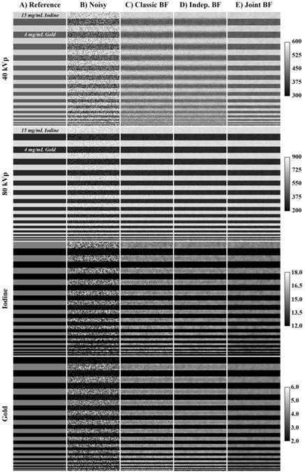
DE decomposition of a 3D digital bar phantom. (A) The central slice through the digital bar phantom with 15 mg/mL iodine in odd rows and 4 mg/mL gold in even rows, a relevant case for in vivo studies. (B) The slice from (A) with 70 HU of zero-mean, white Gaussian. (C) Part (B) denoised with classic BF before decomposition. Edges are well preserved at all frequencies, but substantial noise remains. (D) Part (B) denoised with independent BF before decomposition. Denoising performance is better than Part (C), but edges in the 40 kVp data are noticeably blurred. (E) Denoising of part (B) with the proposed joint BF scheme before decomposition. The results maintain the superior denoising performance of (D) without noticeably blurring the edges in the 40 kVp data. Calibration bars on the far right denote window widths and levels for each row (row 1, 2: HU; row 3, 4: mg/mL). The bar width is 128 voxels (11.3 mm). Line profiles through the central column of each slice can be viewed in the supplemental material: http://www.civm.duhs.duke.edu/AUIsarcoma201211/.

The accuracy of the I and Au maps was then assessed by computing the root-mean-square error (RMSE):

$$\text{RMSE}=\sqrt{\frac{1}{\text{n}}{\sum }_{\text{y}=1}^{\text{n}}{({\left[\text{C}\right]}_{\text{y}}-{\left[\text{C}\right]}_{\text{0}})}^2}$$ (7)

where y indexed the voxels within a given bar, n was the total number of voxels in that bar (n ≥ 128), [C]_y was the measured concentration of C = I or C = Au in voxel y, and where [C]₀ was the expected concentration of I or Au in voxel y. The mean accuracy of the I and Au maps was then computed by averaging the RMSE values over all 900 combinations of I and Au, allowing the mean RMSE to be plotted against the spatial resolution of the different bars. Note that when computing the RMSEs within the I map, for instance, only the bars known to contain I were used to compute the RMSEs because these RMSEs were generally larger than the RMSEs in the corresponding bars which did not contain iodine.

This differs from the contrast-to-noise ratio (CNR) calculions that compared the mean and SDs of the bar known to contain I to the same metrics within the corresponding bar which did not contain I. CNR characterized the detectability of each element within the decomposition maps afforded by the different filtration schemes, and was computed for I and Au as follows:

$$\text{CNR}=\frac{|m_1-m_2|}{\sqrt{{{\sigma }_1}^2+{{\sigma }_2}^2}}$$ (9)

where m1, m₂ and σ₁², σ₂² corresponded to means and variances measured in complementary bars of the I or Au map. The mean detectability of I, for instance, was then computed by averaging the CNR over all spatial resolutions and concentrations of Au (16*30 = 480 samples), allowing the mean CNR to be plotted against concentrations of I. A similar average was computed over all spatial resolutions and concentrations of I to determine the mean detectability of Au. To assess the limits of detectability, the Rose criterion was applied (Rose, 1948), suggesting that a given concentration of I or Au could be reliably detected when the mean CNR was ≥ 5.

2.6. Calibration phantom

To calibrate the sensitivity matrix in Equation 1 and to validate the real-world performance of the filtration scheme chosen using the digital phantom, a physical calibration phantom was constructed. The phantom consisted of a tube of water, representing the body of a rodent, (diameter: 30 mm) surrounded by several smaller vials (diameter: 5.5 or 8 mm; see Figure 5). Four vials contained known concentrations of I: 2, 4, 6, 10 mg/mL. Five vials contained known concentrations of Au: 0.5, 1, 2, 4, 6 mg/mL. One vial contained water and was used to calibrate the HU at each energy because it was presumed less susceptible to beam hardening than the large tube of water. The final three vials contained mixed concentrations of iodine and gold: 1.5, 4.5 mg/mL; 3, 3 mg/mL; and 4.5, 1.5 mg/mL. The complete phantom was scanned using kVp switching, with 250 mA and 16 ms per exposures at 40 kVp and 160 mA, 10 ms per exposure at 80 kVp. In each case, a set of 360 projections was acquired over 360°. The 40 and 80kVp sets were reconstructed with an isotropic voxel size of 88 microns using the Feldkamp algorithm (Feldkamp et al., 1984) and were scaled to HU. The 40 and 80 kVp volumes were registered as previously outlined in Section 2.3 (fixed rotation). The registered volumes were then filtered using joint BF (Equation 5).

Figure 5.

DE decomposition of a physical calibration phantom containing water (A), Au (B), and I (C) with concentrations in mg/mL as shown. Three vials (bottom right of B and C) contained mixtures of both I and Au. Columns 1 and 2 show a corresponding slice through the 80 and 40 kVp data, with the window width and level of the slices designated below (HU). Columns 3 and 4 show the same slice through the I and Au maps with the window width and level of both maps designated below (mg/mL). The scale bar at the bottom right applies to all images in this figure. Results are shown with (row 2) and without (row 1) joint BF.

The filtered phantom was then used to calibrate the sensitivity matrix by defining volumes of interest (VOIs) within each vial. The VOIs were adequately eroded in 3D to avoid partial volume effects around the edges of each vial. After erosion, each VOI contained a minimum of 6.8e4 voxels. This number of voxels from the 0 (water), 2, 4, and 6 mg/mL gold and iodine VOIs were randomly selected and grouped between energies to minimize bias from beam hardening artifacts. The optimal sensitivity matrix was then found by solving the following optimization problem using MATLAB's fminsearch function (The MathWorks, Natick, MA):

$$\begin{array}{c}{min}_{\text{s}}{\Vert \text{C}-{\text{S}}^{-1}\text{H}\Vert }_2^2\\ \text{C}=\left[\begin{array}{c}{\text{C}}_{\text{I}}\\ {\text{C}}_{\text{Au}}\end{array}\right];\text{S}=\left[\begin{array}{cc}{\text{e}}_{\text{I},\text{E}1}& {\text{e}}_{\text{Au},\text{E}1}\\ {\text{e}}_{\text{I},\text{E}2}& {\text{e}}_{\text{Au},\text{E2}}\end{array}\right];\text{H}=\left[\begin{array}{c}{\text{CT}}_{\text{E}1}\\ {\text{CT}}_{\text{E}2}\end{array}\right];{\text{S}}_0\left[\begin{array}{cc}40& 100\\ 50& 70\end{array}\right]\end{array}$$ (11)

where C was the matrix of known concentrations (mg/mL), S was the sensitivity matrix to be optimized (HU/mg/mL), H was the intensity in each voxel at each energy (HU, randomized grouping), and where S₀ was the sensitivity matrix used to initialize the optimization. The optimization was run five times with different random pairings. The average sensitivities from the five optimizations were used to construct and decompose the digital phantoms (Section 2.5) and to perform decomposition of the in vivo data (Section 2.7). The result from Equation 11 was characterized by recording the minimized RMSE over all water, I, and Au voxels included in the optimization. Linear correlation coefficients reporting how well the optimized sensitivities matched mean intensities measured within the I and Au VOIs were also computed. To quantify the real-world performance of joint BF in DE applications, the physical phantom was decomposed with and without joint BF. The precision and accuracy of each decomposition was then assessed by plotting histograms of the voxels within each VOI.

2.7. In vivo tumor imaging

The animal experiment in this study was approved by the Duke University Institutional Animal Care and Use Committee. A soft tissue sarcoma was generated by intramuscular injection of an adenovirus expressing Cre recombinase (Gene Transfer Vector Core, University of Iowa) into a LSL-Kras^G12D; p53^FL/FL compound mutant mouse as described previously (Kirsch et al., 2007). For imaging, the mouse was injected with 0.1 mL/25 g of AuNp via the tail vein. It was then scanned using DE micro-CT at 0 hrs. (day 1), 24 hrs. (day 2), 48 hrs. (day 3), 72 hrs. (day 4), and 120 hrs. (day 6) post AuNp injection. Two scans were conducted on day 4, one prior to and the second immediately following the tail vein injection of 0.4 mL/25 g Lip-I contrast agent. All scans were performed using the same micro-CT system and the same imaging and reconstruction parameters used for the calibration phantom (Section 2.6). The cumulative dose associated with these scans was 0.78 Gy. Registration between the reconstructed 40 and 80 kVp volumes was performed as outlined in Section 2.3 (fixed rotation). Joint BF and DE decomposition were performed with the 40 and 80 kVp volumes from each time point using Equations 5 and 1, respectively. As a preprocessing step for analysis, the sarcoma and the skeleton were manually segmented within each reconstructed data set using Avizo (VSG, Burlington, MA; see details in Moding et al., 2012)).

2.8. Fractional blood volume and vascular permeability

The 3D I and Au maps resulting from decomposition were used to compute two metrics for characterizing tumor vasculature—fractional blood volume (FBV) and vascular permeability. FBV measured the fraction of the tumor volume composed of vasculature and was computed as follows:

$$\begin{array}{c}{\text{C}\prime }_{\text{n}}=\{\begin{array}{cc}0,& {\text{C}}_{\text{n}}\le {\text{C}}_{\text{b}}\\ {\text{C}}_{\text{n}},& {\text{C}}_{\text{n}}>{\text{C}}_{\text{b}}\end{array}\\ \text{FBV}=\frac{1}{\text{N}\ast {\text{C}}_{\text{IV}}}\ast \sum _{\text{n}=1}^{\text{N}}{\text{C}\prime }_{\text{n}}\end{array}$$ (12)

where C_b was the threshold of detectability for each element (1.50 mg/mL Au; 2.24 mg/mL I), C_n and C′_n were the concentrations in voxel n before and after thresholding with C_b, N was the total number of tumor voxels, and where C_IV was the intravascular blood pool concentration of the element of interest measured in the lumen of the descending aorta. FBV was computed on day 1 (immediately after the injection of AuNp) using the Au map and on day 4 (immediately after the injection of Lip-I) using the I map. Because FBV could not be explicitly measured on days 2, 3, and 6, it was estimated using a linear fit.

Accumulated mass (AM) measured the accumulation of a given element within the tumor by extravasation and was computed as follows:

$$\begin{array}{c}{\text{C}\prime }_{\text{n}}=\{\begin{array}{cc}0,& {\text{C}}_{\text{n}}\le {\text{C}}_{\text{b}}\\ {\text{C}}_{\text{n}}-{\text{C}}_{\text{b}},& {\text{C}}_{\text{n}}>{\text{C}}_{\text{b}}\end{array}\\ \text{AM}=\text{v}\ast \sum _{\text{n}=1}^{\text{N}}{\text{C}\prime }_{\text{n}}\end{array}$$ (13)

where v was the volume of a single voxel (6.81e-7 mL). Because extravasated concentrations were close to the threshold of detectability, the threshold was subtracted from all voxels before computing AM.

Given the long circulating nature of the contrast agents used, computing the accumulated mass in the presence of residual blood pool enhancement from the same element required a correction factor. The corrected quantity was called the corrected accumulated mass (CAM) and was computed as follows:

$$\text{CAM}=\text{AM}-\text{FBV}\ast \text{TV}\ast {\text{C}}_{\text{X}}$$ (14)

where TV was the tumor volume (mL), and where AM, FBV, and TV were all measured on the same day and for the same element. C_X was calibrated to day 1 for Au (2.62 mg/mL) and to day 4 (post Lip-I injection) for I (4.71 mg/mL) using the fact that the CAM had to equal zero immediately after injection of the contrast agent:

$${\text{C}}_{\text{X}}=\frac{\text{AM}}{\text{FBV}\ast \text{TV}}$$ (15)

On days 2, 3, and 6, CAM was computed as follows:

$$\text{CAM}=\text{AM}-\text{FBV}\ast \text{TV}\ast \frac{{\text{C}}_{\text{IV},\text{curr}}‒{\text{C}}_{\text{b}}}{{\text{C}}_{\text{IV},\text{ref}}‒{\text{C}}_{\text{b}}}{\text{C}}_{\text{X}}$$ (16)

where C_X was the calibrated value on day 1 (Au) or day 4 (I) and where (C_IV,curr − C_b)/(C_IV,ref − C_b) was the ratio of the current blood pool concentration to the blood pool concentration at the time point when C_X was measured. Note that Equation 16 reduced to Equation 14 on day 1 for Au and on day 4 for I (i.e. when C_IV,curr = C_IV,ref) and that the CAM (Equation 16) reduced to the AM (Equation 13) when the residual blood pool enhancement dropped below the threshold of detectability (i.e. when C_IV,curr = C_b). To allow comparison of the extravasation between days in the presence of tumor growth, the corrected accumulated concentration (CAC) was computed by normalizing the CAM by the TV:

$$\text{CAC}=\frac{\text{CAM}}{\text{TV}}$$ (17)

3. Results

3.1. Digital phantom studies

Figure 2 illustrates the digital bar phantom and provides a visual comparison of the central slice of the phantom after the addition of noise and then after filtration with classic, independent, or joint BF. Specifically, the figure shows the 40 and 80 kVp versions of the phantom and their respective decompositions for a representative combination of Au and I (4 and 15 mg/mL, respectively; models the in vivo case of extravasated Au and vascular I). The SDs in the decomposed I and Au maps were roughly proportional to the SDs in the 40 kVp data, the energy at which the contrast between the two materials was lowest (137 HU vs. 511 HU at 80 kVp). The SDs measured at the lowest spatial resolution (0.36 lp/mm) for the 40 kVp (odd bar), 80 kVp (odd bar), I (odd bar), and Au (even bar) data are presented in Table 1. Expanding this analysis to all combinations of I and Au and to finer spatial resolutions where filtration can introduce significant bias, Figure 3 summarizes mean RMSEs measured in the I and Au maps after decomposition of the noisy and filtered versions of the phantom. As expected, the mean RMSEs for both materials remained constant across all spatial resolutions when decomposing the noisy data (I: 3.1 mg/mL; Au: 1.6 mg/mL). In general, all three forms of BF greatly improved the mean RMSEs across all relevant spatial resolutions relative to the unfiltered decompositions, with joint BF yielding the best overall performance. Similarly, the mean limits of detectability were analyzed for each material. Figure 4 plots the mean I and Au CNRs against concentrations of I (A) and Au (B), respectively. The limits of detectability (mean CNR = 5) are summarized in Table 2. Again, joint BF is seen to outperform the other filtration schemes tested with a detectability limit of 2.3 mg/mL (18 mM) for I and 1.0 mg/mL (5.1 mM) for Au.

Table 1.

Standard deviations at 0.36 lp/mm.

Component	Noisy	Classic BF	Indep. BF	Joint BF
40 kVp (HU)	71.77	20.44	13.99	5.19
80 kVp (HU)	70.54	15.46	10.02	9.45
Iodine (mg/mL)	3.20	0.77	0.33	0.33
Gold (mg/mL)	1.65	0.48	0.23	0.14

Figure 3.

Changes in denoising performance with spatial resolution for each type of filtration applied to the digital bar phantom. (A) Mean RMSEs in the I decomposition over all tested concentrations of I and Au and over all relevant spatial resolutions. (B) Mean RMSEs in the gold decomposition, again averaged over all tested concentrations of I and Au. Note that joint filtration consistently outperforms classic and independent filtration. Cubic interpolation was used to connect sampled points.

Figure 4.

Changes in mean contrast-to-noise ratio (CNR) with concentration. (A) Mean CNR in the I decomposition over all tested concentrations of Au and over all spatial resolutions. (B) Mean CNR in the Au decomposition over all tested concentrations of I and over all spatial resolutions. Gray boxes denote the region of uncertainty in accordance with the Rose criterion (i.e. CNR ≤ 5). The independent and joint BF schemes improve the limits of detectability for I and Au by more than a factor two relative to classic BF. Cubic interpolation was used to connect sampled points.

Table 2.

Limits of detectability (mean CNR = 5).

Component	Noisy	Classic BF	Indep. BF	Joint BF
Iodine (mg/mL)	22.3	8.2	3.3	2.3
Gold (mg/mL)	N/A	4.0	1.3	1.0

3.2. Calibration phantom

Given the success of joint filtration, Figure 5 shows a slice through the 80 and 40 kVp reconstructions of the calibration phantom, as well as the same slices after joint filtration. Following the optimization scheme outlined in Section 2.6, the optimum sensitivity matrix, S_opt, was the following:

$${\text{S}}_{\text{opt}}=\left[\begin{array}{cc}{\text{e}}_{\text{I},\text{E}1}& {\text{e}}_{\text{Au},\text{E}1}\\ {\text{e}}_{\text{I},\text{E}2}& {\text{e}}_{\text{Au},\text{E}2}\end{array}\right]=\left[\begin{array}{cc}36.36& 102.00\\ 53.56& 73.16\end{array}\right]$$ (18)

This resulted in a minimum RMSE of 0.55 mg/mL. Repeating the optimization yielded SDs of less than 0.05 HU/mg/mL for the individual sensitivities. Using S_opt, the linear correlation coefficients (R²) between the mean intensities measured in the 0 (water), 2, 4, and 6 mg/mL Au and I vials and the optimized sensitivities were 0.99 for I at 40 kVp and 1.00 for I at 80 kVp, Au at 80 kVp, and for Au at 40 kVp, confirming that S_opt was indeed optimal for decomposing each material and each energy. Figure 6 summarizes the results of decomposing the calibration phantom and graphically illustrates the means and SDs of the decomposition results relative to the expected values (vertical, dashed lines). Performing decomposition without filtration (A) is seen to yield extremely broad peaks with low precision but relatively high accuracy (similar results for Au not shown). Performing decomposition after joint BF (B, C, D) is seen to improve precision by ∼4 times while maintaining accuracy.

Figure 6.

Summary of decomposition accuracy in the physical water, iodine, and gold calibration phantom. (A) A histogram representing the distribution of decomposed concentrations of I in the I only vials without filtration and by expected concentration (mg/mL). The y-axis denotes the fraction of voxels at each concentration (6.8e4 total voxels per concentration). Dashed vertical lines denote the expected concentrations. (B) A repeat of (A) using the jointly filtered data. Note the change in scale on the x-axis. (C) An analogous plot to (B) for the Au only vials. (D) Histograms of I and Au voxels from the I and Au decompositions, respectively, within the mixed vials (see Figure 5).

3.3. In vivo tumor imaging

Figure 7 illustrates the real-world performance of joint BF when applied to the in vivo data (day 4, post Lip-I injection). While the purpose of this paper is generally to improve the accuracy and limits of detectability within DE decompositions, column C clearly shows that joint BF provides homogenous denoising performance within the grayscale data at each energy. Given the previously discussed relationship between the regression function K(y) used to improve denoising performance (Equation 4) and the MTF, it is not surprising that parts of the bone (enhancement >2000 HU) are noticeably smoothed (black arrows). Close inspection also reveals slight smoothing of the boundary between tissue and the surrounding air. Overall, however, the mean and SD within these difference images denoted very strong denoising performance with minimal overall bias (mean ± SD): 1.41 ± 68.6 HU (80 kVp), 1.09 ± 62.6 HU (40 kVp). Like the digital phantom (Figure 4) and the calibration phantom (Figure 5), the CNR of each elemental map of the in vivo data dramatically improved after filtration (Figure 7D, E).

Figure 7.

Application of joint BF to in vivo data acquired immediately after the injection of Lip-I on day 4. (A) Matching coronal slices through the reconstructed 80 and 40 kVp data sets (noise SD: ∼70 HU). Note the visual ambiguity between iodine and gold contrast. (B) The slices from (A) after joint BF (σ_w = 70 HU, m = 2). (C) The difference before and after filtration: (A)-(B). Black arrows indicate bones which are noticeably compromised by the denoising process. White arrows indicate the location of the primary sarcoma. (D) DE decomposition using the noisy slices from (A). (E) Identical DE decomposition using the filtered slices from (B). Note that the bones (shown in white) where segmented and excluded from the decomposition. The scale bar at the bottom right of (E) applies to all images. The two calibration bars at the bottom left denote the window widths and levels in HU for columns (A) and (B) and for column (C), respectively. The calibration bars at the bottom right denote the window widths and levels in mg/mL for I and Au, respectively, in (D) and (E). The filtered data sets shown in this figure (B, E) can be downloaded from the supplemental material: http://www.civm.duhs.duke.edu/AUIsarcoma201211/.

Figure 8 focuses on the soft-tissue sarcoma itself, summarizing the results of the in vivo animal experiment by showing maximum intensity projections (MIPs) through the segmented tumor at each day the tumor was scanned. The day 1 scan, immediately following the injection of AuNp, highlights the vasculature within the tumor. Already by day 2, most of the AuNp have extravasated from the vasculature into the surrounding tumor. The day 4 Au map remains roughly constant before and after the Lip-I injection. Using DE decomposition, the addition of Lip-I allowed simultaneous measurement of tumor FBV and vascular permeability. On day 6, both the AuNp and the Lip-I have extravasated from the tumor vasculature into the surrounding tumor; however, the extravasation patterns of the two materials are markedly different. Figure 9 quantifies these observations. Over the course of 5 days, the tumor volume is seen to increase by 35%, with a noticeable increase in tumor volume after the injection of Lip-I on day 4. As visually observed in Figure 8, the uptake of the AuNp occurs most rapidly between day 1 and day 2. Furthermore, the CAC of Au within the tumor is seen to increase after the injection of Lip-I. Given that the tumor continues to grow and no additional AuNp were injected, we suspect this is caused by beam-hardening artifacts introduced by highly attenuating combinations of I and Au. Note that our recent work (Moding et al., 2012) provides validation for our CT-derived fractional blood volume and permeability measurements using standard immunohistochemistry.

Figure 8.

In vivo characterization of a primary soft-tissue sarcoma using DE micro-CT. This matrix provides a visual representation of the data acquired on day 1 (AuNp injection), day 2, day 3, day 4 (pre Lip-I injection), day 4 (post Lip-I injection), and on day 6 and illustrates the ability to simultaneously decompose I and Au in vivo. The columns represent the 40 kVp data, the 80 kVp data, the I map, the Au map, and the superposition of the I and Au maps. Each panel is a MIP through the segmented tumor at the designated day. White arrows denote an apparent increase in Au concentration within the vasculature after the injection of Lip-I on day 4. Calibration bars at the upper right denote the window widths and levels in HU for the 40 kVp and 80 kVp data and in mg/mL for I and Au maps. The scale bar at the bottom right applies to all panels. An animated supplement to this figure is available in the supplemental material: http://www.civm.duhs.duke.edu/AUIsarcoma201211/.

Figure 9.

Tumor growth and elemental accumulation. (A) Tumor volume measured by manual segmentation on days 1, 2, 3, 4, and 6. Note the injection of the Lip-I on day 4 causes a noticeable increase in volume. (B) The extravasated concentrations (CACs) of I and Au measured on the same days. Note the correction process (Equation 15) calibrates the extravasated concentration to zero on the day of injection.

4. Discussion

Spectral CT imaging is expected to play a major role in the diagnostic arena as it can provide quantitative elemental maps. One fascinating possibility is the ability to discriminate multiple contrast agents targeting different biological sites. In this paper we have established methods which allow in vivo discrimination of I and Au contrast using DE micro-CT. We have tailored this approach to quantify two important vascular biomarkers in cancer, FBV and vascular permeability. In a recent publication (Moding et al., 2012), we used DE micro-CT to assess vascular effects caused by radiation treatment on primary soft-tissue sarcomas in mice. A major limitation of that study was the use of a single contrast agent (Lip-I), requiring the assumption of constant FBV over time to separate intra-vascular and extra-vascular concentrations. This study provides an elegant solution to this problem by using two types of nanoparticles based on Au and I.

When separating mixtures of I and Au by DE decomposition, joint BF was seen to be an excellent denoising algorithm for improving the results. It provided superior decomposition accuracy, precision, and elemental detectability relative to unfiltered data and to related filtration schemes which did not exploit spectral correlation in both phantom studies and in vivo data. While we did not exhaustively compare all possible combinations of smoothing parameters for the range weighting (Equations 3 and 6) and regression kernel (Equation 4), it is expected that the conclusions drawn here regarding the relative performance of joint BF in spectral CT applications are generally applicable for several reasons. First, the choice of domain and range weighting functions used here was based on brute-force optimizations of BF using similar data as documented in (Clark et al., 2012). Second, we previously demonstrated the superiority of BF to Gaussian smoothing and median filtration using our grayscale CT data (Clark et al., 2012) and in DE applications (Badea et al., 2012). Here, building on the conclusions in these papers, joint BF is seen to outperform classic BF. Implicitly, we do make the assumption that the regression kernel always improves filter performance relative to classic BF; however, we back up this assumption by calibrating the kernel relative to the MTF of our imaging system and by explicitly testing both independent filtration and joint filtration, showing that each component contributes to the improvement of filter performance. Given these conclusions, we are excited by the possibilities of applying joint BF to other spectral applications such as dose reduction in DE-CT relative to the levels of a single diagnostic scan and co-filtering data sets acquired at more than two energies (e.g. data acquired with photon counting detectors, attempting to separate more than two materials).

Here, we took the first steps toward these exciting applications. Using a digital bar phantom, optimized scanning energies, and an optimized sensitivity matrix, we determined the limits of detectability for I and Au to be 2.3 and 1.0 mg/mL, respectively. Comparing these limits with the thresholds of detectability empirically determined using in vivo data decomposed with the same sensitivity matrix (2.24 mg/mL I, 1.50 mg/mL Au), the digital bar phantom experiments are seen to accurately emulate the filter performance using in vivo data, validating the results of the digital phantom experiments. The in vivo and digital phantom experiments are further validated by the decomposition of the calibration phantom (Figure 5), in which the vials containing 1 mg/mL of Au and 2 mg/mL of I are clearly visible relative to the water at the center of the phantom, a distinction that cannot be made in the unfiltered decompositions. Perhaps most importantly, the notion of separating two exogenous contrast agents with high sensitivity is validated by accurately separating mixtures of iodine and gold near the limits of detectability within the calibration phantom.

There is, however, one notable difference between the digital phantom experiments and the in vivo experiment. The digital phantom experiments did not simulate the effects of beam hardening, effects which can be significant for the concentrations of I and Au observed in vivo (i.e. enhancements ≥ 500 HU). For this reason, the optimal sensitivity matrix was calibrated using low to intermediate concentrations of I and Au (0, 2, 4, 6 mg/mL) which were presumed to be least affected by beam hardening. In practice, calibrating the sensitivities with higher concentrations yields uniformly lower sensitivities for I and Au at 40 and 80 kVp as documented in (Badea et al., 2011). As a consequence of the choice to optimize the sensitivity matrix for low to intermediate concentrations, the sensitivity matrix derived here is better conditioned than the sensitivity matrix previously derived, improving the accuracy in separating I and Au, particularly near the limits of detectability of the two materials. It should be noted that there is another source of the difference between the sensitivities derived here and the sensitivities derived in (Badea et al., 2011). Sensitivities derived here were chosen to minimize aggregate decomposition errors for both I and Au in a least-squares sense (Equation 11), whereas the cited paper minimized the decomposition error for each material and energy independently (i.e. linear fitting of enhancement vs. concentration). For this study, a potential additional source of decomposition errors similar to beam hardening, cross-scattering, was avoided by using a single-source kVp switching acquisition protocol instead of a dual-source acquisition protocol.

Given the choices made in calibrating the sensitivity matrix, beam hardening manifested itself as a slight bias in measuring higher concentrations of I, as illustrated in the 10 mg/mL distribution in Figure 6B (calibration phantom). Another example can be seen in the in vivo data immediately after the injection of Lip-I on day 4 (Figure 8, white arrows). Because beam hardening affects the measured intensity of I in the vasculature, it appears as though there is also a small concentration of Au in the vasculature which is not seen before the injection of Lip-I. In Figure 9B, this bias manifests itself as an artificial increase in the CAC of Au after the injection of Lip-I. Fortunately, the magnitude of this bias is relatively small compared with the magnitude of the CAC before the injection of Lip-I (CAC Au = 0.63 mg/mL before, 0.68 mg/mL after). Note that we may be able to control the magnitude of this bias in future experiments by injecting lower volumes of Lip-I and AuNp, a luxury afforded by our robust limits of detectability and a choice which may also be physiologically favorable.

Another important choice regarding the in vivo experiments was to image the same mouse six times over the course of five days, resulting in a cumulative, longitudinal dose of 0.78 Gy. Although this dose may not impact preclinical experiments using soft-tissue sarcomas in mice, the radiation exposure from six DE scans would not be appropriate in clinical applications. In the feasibility studies presented here, the number of scans was motivated by the desire to illustrate the time course of Au and I extravasation and to use these measurements to validate consistency in the computation of FBV and CAC. Once the mechanisms of extravasation have been accurately characterized for a given tumor model, most follow-up studies designed to characterize tumor FBV and permeability will only require two DE scans, one to compute the FBV of Au immediately after injection and a second to compute the CAC of Au and the FBV of I at a later time point. This paradigm is an extension of the one used in our recent study on the effects of radiation treatment on tumor vasculature (Lip-I only; see Moding et al., 2012) which had an associated dose of 0.26 Gy per mouse.

5. Conclusions

DE micro-CT using two types of nanoparticles based on I and Au provides a very elegant and effective tool for non-invasive assessment of vascular changes in tumors, particularly when paired with joint BF to improve the limits of detectability for each element. Such an approach has broad applicability in characterizing tumors and in monitoring their response to treatment (e.g. radiation therapy, anti-angiogenic drugs). It also opens the door for hybrid protocols combining drug delivery with contrast localization by exploiting the unique properties of nanoparticles such as liposomes (Karathanasis et al., 2009). Because of the similarities between our DE micro-CT system and clinical DE systems (i.e. high-flux polychromatic x-ray sources, similar acquisition strategies), we believe that successful development of our imaging methods can be translated into the clinic. Moreover, by successfully overcoming the challenges of using DE micro-CT with small animals (i.e. higher resolutions and noise levels), the novel and robust methods that we develop preclinically have the potential to be even more robust when applied in clinic applications.

References

- Badea C, Johnston S, Johnson B, De Lin M, Hedlund LW, Johnson GA. A dual micro-CT system for small animal imaging. In: Hsieh JS, Ehsan, editors. Proc SPIE, Medical Imagin. San Diego, CA: SPIE; 2008a. pp. 691342–10. [DOI] [PMC free article] [PubMed] [Google Scholar]
- Badea C, Johnston S, Qi Y, Ghaghada K, Johnson G. Dual-energy micro-CT imaging for differentiation of iodine-and gold-based nanoparticles. Proc SPIE. 2011;7961:79611X. [Google Scholar]
- Badea CT, Drangova M, Holdsworth DW, Johnson GA. In vivo small-animal imaging using micro-CT and digital subtraction angiography. Physics in Medicine and Biology. 2008b;53:R319–50. doi: 10.1088/0031-9155/53/19/R01. [DOI] [PMC free article] [PubMed] [Google Scholar]
- Badea CT, Guo X, Clark D, Johnston SM, Marshall CD, Piantadosi CA. Dual-energy micro-CT of the rodent lung. American Journal of Physiology Lung Cellular and Molecular Physiology. 2012;302:L1088–97. doi: 10.1152/ajplung.00359.2011. [DOI] [PMC free article] [PubMed] [Google Scholar]
- Boote E, Fent G, Kattumuri V, Casteel S, Katti K, Chanda N, Kannan R, Katti K, Churchill R. Gold nanoparticle contrast in a phantom and juvenile swine: models for molecular imaging of human organs using x-ray computed tomography. Academic Radiology. 2010;17:410–7. doi: 10.1016/j.acra.2010.01.006. [DOI] [PMC free article] [PubMed] [Google Scholar]
- Chanda N, Shukla R, Zambre A, Mekapothula S, Kulkarni RR, Katti K, Bhattacharyya K, Fent GM, Casteel SW, Boote EJ, Viator JA, Upendran A, Kannan R, Katti K. An effective strategy for the synthesis of biocompatible gold nanoparticles using cinnamon phytochemicals for phantom CT imaging and photoacoustic detection of cancerous cells. Pharmaceutical Research. 2011;28:279–91. doi: 10.1007/s11095-010-0276-6. [DOI] [PubMed] [Google Scholar]
- Clark D, Johnson G, Badea C. Proc SPIE. 2012. Denoising of 4D cardiac micro-CT data using median-centric bilateral filtration; pp. 83143Z-Z–12. [DOI] [PMC free article] [PubMed] [Google Scholar]
- Cormode DP, Roessl E, Thran A, Skajaa T, Gordon RE, Schlomka JP, Fuster V, Fisher EA, Mulder WJM, Proksa R, Fayad ZA. Atherosclerotic plaque composition: analysis with multicolor CT and targeted gold nanoparticles. Radiology. 2010;256:774–82. doi: 10.1148/radiol.10092473. [DOI] [PMC free article] [PubMed] [Google Scholar]
- Feldkamp LA, Davis LC, Kress JW. Practical cone-beam algorithm. J Opt Soc Am. 1984;1:612–19. [Google Scholar]
- Ghaghada KB, Badea CT, Karumbaiah L, Fettig N, Bellamkonda RV, Johnson GA, Annapragada A. Evaluation of tumor microenvironment in an animal model using a nanoparticle contrast agent in computed tomography imaging. Academic Radiology. 2011;18:20–30. doi: 10.1016/j.acra.2010.09.003. [DOI] [PMC free article] [PubMed] [Google Scholar]
- Ghann WE, Aras O, Fleiter T, Daniel MC. Syntheses and characterization of lisinopril-coated gold nanoparticles as highly stable targeted CT contrast agents in cardiovascular diseases. Langmuir : the ACS Journal of Surfaces and Colloids. 2012;28:10398–408. doi: 10.1021/la301694q. [DOI] [PubMed] [Google Scholar]
- Guo X, Johnston SM, Johnson GA, Badea CT. A comparison of sampling strategies for dual energy micro-CT. Proceedings of SPIE. 2012;8313:831332. [Google Scholar]
- Hainfeld JF, Slatkin DN, Focella TM, Smilowitz HM. Gold nanoparticles: a new X-ray contrast agent. The British Journal of Radiology. 2006;79:248–53. doi: 10.1259/bjr/13169882. [DOI] [PubMed] [Google Scholar]
- Jackson PA, Rahman WN, Wong CJ, Ackerly T, Geso M. Potential dependent superiority of gold nanoparticles in comparison to iodinated contrast agents. European Journal of Radiology. 75:104–9. doi: 10.1016/j.ejrad.2009.03.057. [DOI] [PubMed] [Google Scholar]
- Jeswani T, Padhani AR. Imaging tumour angiogenesis. Cancer imaging : the official publication of the International Cancer Imaging Society. 2005;5:131–8. doi: 10.1102/1470-7330.2005.0106. [DOI] [PMC free article] [PubMed] [Google Scholar]
- Johnston S, Johnson GA, Badea CT. Geometric calibration for a dual tube/detector micro-CT system. Medical Physics. 2008;35:1820–9. doi: 10.1118/1.2900000. [DOI] [PMC free article] [PubMed] [Google Scholar]
- Kappler S, Hölzer S, Kraft E, Stierstorfer K, Flohr T. Proc SPIE. 2011. Quantum-counting CT in the regime of countrate paralysis: introduction of the pile-up trigger method; p. 79610T. [Google Scholar]
- Karathanasis E, Suryanarayanan S, Balusu SR, McNeeley K, Sechopoulos I, Karellas A, Annapragada AV, Bellamkonda R. Imaging nanoprobe for prediction of outcome of nanoparticle chemotherapy by using mammography. Radiology. 2009;250:398–406. doi: 10.1148/radiol.2502080801. [DOI] [PubMed] [Google Scholar]
- Kirsch DG, Dinulescu DM, Miller JB, Grimm J, Santiago PM, Young NP, Nielsen GP, Quade BJ, Chaber CJ, Schultz CP, Takeuchi O, Bronson RT, Crowley D, Korsmeyer SJ, Yoon SS, Hornicek FJ, Weissleder R, Jacks T. A spatially and temporally restricted mouse model of soft tissue sarcoma. Nat Med. 2007;13:992–7. doi: 10.1038/nm1602. [DOI] [PubMed] [Google Scholar]
- Kozin SV, Duda DG, Munn LL, Jain RK. Neovascularization after irradiation: what is the source of newly formed vessels in recurring tumors? Journal of the National Cancer Institute. 2012;104:899–905. doi: 10.1093/jnci/djs239. [DOI] [PMC free article] [PubMed] [Google Scholar]
- Libutti SK, Paciotti GF, Byrnes AA, Alexander HR, Jr, Gannon WE, Walker M, Seidel GD, Yuldasheva N, Tamarkin L. Phase I and pharmacokinetic studies of CYT-6091, a novel PEGylated colloidal gold-rhTNF nanomedicine. Clinical Cancer Research. 2010;16:6139–49. doi: 10.1158/1078-0432.CCR-10-0978. [DOI] [PMC free article] [PubMed] [Google Scholar]
- Maeda H. The enhanced permeability and retention (EPR) effect in tumor vasculature: the key role of tumor-selective macromolecular drug targeting. Advances in Enzyme Regulation. 2001;41:189–207. doi: 10.1016/s0065-2571(00)00013-3. [DOI] [PubMed] [Google Scholar]
- Moding EJ, Clark DP, Qi Y, Li YY, Ma Y, Ghaghada K, Johnson GA, Kirsch DG, Badea CT. Dual energy micro-CT imaging of radiation-induced vascular changes in primary mouse sarcomas. International Journal of Radiation Oncology Biology Physics. 2012;1:03635–8. doi: 10.1016/j.ijrobp.2012.09.027. [DOI] [PMC free article] [PubMed] [Google Scholar]
- Mukundan S, Ghaghada K, Badea C, Hedlund L, Johnson G, Provenzale J, Bellamkonda R, Annapragada A. A nanoscale, liposomal contrast agent for preclincal microCT imaging of the mouse. AJR. 2006;186:300–7. doi: 10.2214/AJR.05.0523. [DOI] [PubMed] [Google Scholar]
- Peng C, Zheng L, Chen Q, Shen M, Guo R, Wang H, Cao X, Zhang G, Shi X. PEGylated dendrimer-entrapped gold nanoparticles for in vivo blood pool and tumor imaging by computed tomography. Biomaterials. 2012;33:1107–19. doi: 10.1016/j.biomaterials.2011.10.052. [DOI] [PubMed] [Google Scholar]
- Popovtzer R, Agrawal A, Kotov NA, Popovtzer A, Balter J, Carey TE, Kopelman R. Targeted gold nanoparticles enable molecular CT imaging of cancer. Nano Lett. 2008;8:4593–6. doi: 10.1021/nl8029114. [DOI] [PMC free article] [PubMed] [Google Scholar]
- Rabin O, Manuel Perez J, Grimm J, Wojtkiewicz G, Weissleder R. An X-ray computed tomography imaging agent based on long-circulating bismuth sulphide nanoparticles. Nature materials. 2006;5:118–22. doi: 10.1038/nmat1571. [DOI] [PubMed] [Google Scholar]
- Reuveni T, Motiei M, Romman Z, Popovtzer A, Popovtzer R. Targeted gold nanoparticles enable molecular CT imaging of cancer: an in vivo study. International Journal of Nanomedicine. 2011;6:2859–64. doi: 10.2147/IJN.S25446. [DOI] [PMC free article] [PubMed] [Google Scholar]
- Rose A. The sensitivity performance of the human eye on an absolute scale. J Opt Soc Am. 1948;38:196–208. doi: 10.1364/josa.38.000196. [DOI] [PubMed] [Google Scholar]
- Schlomka JP, Roessl E, Dorscheid R, Dill S, Martens G, Istel T, Baumer C, Herrmann C, Steadman R, Zeitler G, Livne A, Proksa R. Experimental feasibility of multi-energy photon-counting K-edge imaging in pre-clinical computed tomography. Physics in Medicine and Biology. 2008;53:4031–47. doi: 10.1088/0031-9155/53/15/002. [DOI] [PubMed] [Google Scholar]
- Schwickert HC, Stiskal M, Roberts TP, van Dijke CF, Mann J, Muhler A, Shames DM, Demsar F, Disston A, Brasch RC. Contrast-enhanced MR imaging assessment of tumor capillary permeability: effect of irradiation on delivery of chemotherapy. Radiology. 1996;198:893–8. doi: 10.1148/radiology.198.3.8628889. [DOI] [PubMed] [Google Scholar]
- Takeda H, Farsiu S, Milanfar P. Kernel regression for image processing and reconstruction. IEEE Transactions on Image Processing. 2007;16:349–66. doi: 10.1109/tip.2006.888330. [DOI] [PubMed] [Google Scholar]
- Tomasi C, Manduchi R. Bilateral filtering for gray and color images. Sixth International Conference on Computer Vision. 1998:839–46. [Google Scholar]
- Wyss C, Schaefer SC, Juillerat-Jeanneret L, Lagopoulos L, Lehr HA, Becker CD, Montet X. Molecular imaging by micro-CT: specific E-selectin imaging. European Radiology. 19:2487–94. doi: 10.1007/s00330-009-1434-2. [DOI] [PubMed] [Google Scholar]
- Xi D, Dong S, Meng X, Lu Q, Meng L, Ye J. Gold nanoparticles as computerized tomography (CT) contrast agents. RSC Advances 2012 [Google Scholar]
Associated Data
This section collects any data citations, data availability statements, or supplementary materials included in this article.