A Pure L1-norm Principal Component Analysis

Abstract

The L₁ norm has been applied in numerous variations of principal component analysis (PCA). L₁-norm PCA is an attractive alternative to traditional L₂-based PCA because it can impart robustness in the presence of outliers and is indicated for models where standard Gaussian assumptions about the noise may not apply. Of all the previously-proposed PCA schemes that recast PCA as an optimization problem involving the L₁ norm, none provide globally optimal solutions in polynomial time. This paper proposes an L₁-norm PCA procedure based on the efficient calculation of the optimal solution of the L₁-norm best-fit hyperplane problem. We present a procedure called L₁-PCA* based on the application of this idea that fits data to subspaces of successively smaller dimension. The procedure is implemented and tested on a diverse problem suite. Our tests show that L₁-PCA* is the indicated procedure in the presence of unbalanced outlier contamination.

3 Introduction

Principal component analysis (PCA) is a data analysis technique with various uses including dimensionality reduction, quality control, extraction of interpretable derived variables, and outlier detection [15]. Traditional PCA, hereafter referred to as L₂-PCA, is based on the L₂ norm. Principal component analysis using L₂-PCA possesses several important properties such as: the loadings vectors are the eigenvectors of the covariance matrix, the loadings vectors are the successive orthogonal directions of maximum (or minimum) variation in data, and the principal components define the L₂-norm best-fit linear subspaces to the data [15]. The simultaneous occurrence of these properties is unique to L₂-PCA, and is a reason why it is widely-used. The term “pure” in this paper is used to reflect the fact that the proposed L₁-norm PCA shares an analogous property to L₂-PCA in that the principal components are defined by successive L₁-norm best-fit subspaces.

L₂-PCA is sensitive to outlier observations. This sensitivity is the principal reason for exploring alternative norms. Procedures for PCA that involve the L₁ norm have been developed to increase robustness [12, 4, 17, 1, 7, 10, 13, 19]. Galpin and Hawkins [12] develop a robust L₁ covariance estimation procedure. Others have considered robust measures of dispersion for finding directions of maximum variation [8, 7, 19]. The approaches in [8] and [7] are based on the projection pursuit method introduced in [20].

Several previous works involve the L₁ norm in subspace estimation with PCA. Baccini et al. [4] and Ke and Kanade [17] consider the problem of finding a subspace such that the sum of L₁ distances of points to the subspace is minimized, and propose heuristic schemes that approximate the subspace. In light of the camera resectioning problem from computer vision, Agarwal et al. [1] formulate the problem of L₁ projection as a fractional program and give a branch-and-bound algorithm for finding solutions. Gao [13] proposes a probabilistic Bayesian approach to estimating the best L₁ subspace under the assumption that the noise follows a Laplacian distribution.

Measuring error for PCA using the L₁ norm can impart desirable properties besides providing robustness to outlier observations. For example, the L₁ norm is the indicated measure in a noise model where the error follows a Laplace distribution [1, 13]. In special applications such as cellular automata models, where translations can only occur along unit directions, the fit of a subspace can be measured using the L₁ norm [5, 18].

In this paper, we propose a new approach for robust PCA, L₁-PCA*, based on a “pure” application of the L₁ norm in the sense that it uses globally optimal subspaces that minimize the sum of L₁ distances of points to their projections. L₁-PCA* generates a sequence of subspaces, projecting data down one dimension at a time, in a manner analogous to L₂-PCA. The procedure makes use of a polynomial-time algorithm for projecting m-dimensional data into an L₁-norm best-fit (m − 1)-dimensional subspace. The algorithm is based on results concerning properties of L₁ projection and best-fit hyperplanes [25, 22, 21, 5]. The provable optimality of the projected subspace ensures that interesting properties are inherited. The polynomiality of the algorithm makes it practical. We establish experimentally conditions under which the proposed procedure is preferred over L₂-PCA and other previously-investigated schemes for robust PCA.

4 L₁ regression, geometry of the L₁ norm, and best-fit subspaces

Linear regression models seek to find a hyperplane of the form

$$y={\beta }_0+{\beta }^{T}x$$

for a dependent variable y and independent variables x. In L₂ regression, the hyperplane of best fit is determined for a given data set (y_i, x_i), i = 1, … , n by minimizing the residual sum of squared errors given by

$$\sum _{i=1}^n{(y_i-({\beta }_0+{\beta }^T{x}_i))}^2.$$

In L₂ regression, the distance of points to the fitted hyperplane is given by the L₂ norm. L₁ linear regression is analogous to L₂ regression in that they both find a hyperplane that minimizes the sum of distances of points to their projections along the unit direction defined by the dependent variable. In the case of L₁ regression, the distances are measured using the L₁ norm. The sum of absolute errors is minimized. A standard result about L₁ regression is that the hyperplane can be found by solving a linear program (LP) [6, 26]. The L₁ regression LP is as follows.

$${\beta }_0,\stackrel{\min }{\beta ,e^{+},e^{-}}\sum _{i=1}^n{e}_i^{+}+e_i^{-},$$ (R)

subject to

$$\begin{array}{cc}\hfill {\beta }_0+{\beta }^T{x}_i+e_i^{+}-e_i^{-}& =y_i,i=1,\dots ,n,\hfill \\ \hfill e_i^{+},e_i^{-}& \ge 0,i=1,\dots ,n.\hfill \end{array}$$

The input data are $x_i\in {\mathbb{R}}^m$, i = 1, …, n which are rows of the data matrix $X\in {\mathbb{R}}^{n\times m}$, and the dependent variable values y_i, i = 1, …, n. The vector β in (R) are the regression coefficients and the variable β₀ is the level value that are to be determined by the optimal solution to the LP. The variables $e_i^{+}$ and $e_i^{-}$ are the errors measured as the distance from either side of the hyperplane to observation i. Note that at most one of each pair $e_i^{+}$, $e_i^{-}$ is positive at optimality, and the sum of absolute errors is ${\Sigma }_{i=1}^n(e_i^{+}+e_i^{-})$.

Given an m × q matrix A, the internal (linear combination of points) representation of a subspace defined by A is the column space of A, given by $\mathcal{C}\left(A\right)=\{z\in {\mathbb{R}}^m\mid A\lambda =z\text{for all}\lambda \in {\mathbb{R}}^q\}$. The external (intersection of hyperplanes) representation is ${\mathcal{C}}^{\prime }\left(A\right)=\{z\in {\mathbb{R}}^m\mid A^{T}z=0\}$.

The projection of a point $x\in {\mathbb{R}}^m$ on a set S is the set of points P ⊆ S such that the distance between x and points in S is minimized. Distance for PCA is usually measured using the L₂ norm. The L₂ norm of a vector x is

$${\mid \mid x\mid \mid }_2=\sqrt{\sum _{i=1}^m{x}_i^2}.$$

When S is an affine set, the L₂ projection of x is a unique point and the direction from P to x orthogonal to S.

The L₁ norm of a vector x is

$${\mid \mid x\mid \mid }_1=\sum _{i=1}^m\mid x_i\mid .$$

Using the L₁ norm for measuring distance results in different projections. Figure 1 illustrates this difference for the case when $x\in {\mathbb{R}}^2$ and S is a line. The figure represents the level sets using the L₁ and L₂ norms. The L₂ norm level sets in two dimensions are circles; the L₁ norm level sets are diamonds. Notice that the L₁ projection occurs along a horizontal direction. The property that projections occur along a single unit direction generalizes to multiple dimensions [21, 5]. Further, the direction of a projection depends only on the orientation of the hyperplane and not on the location of the point [21]. These two properties lead to the following result about L₁-norm best-fit hyperplanes; that is, hyperplanes for which the sum of L₁ distances of points to their projections is minimized.

Figure 1.

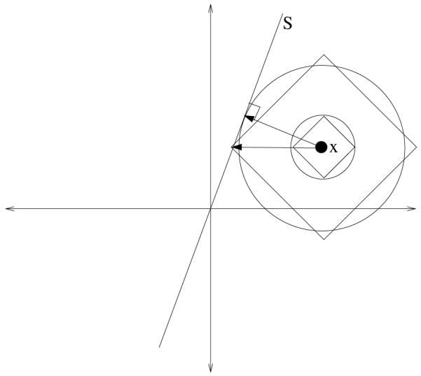
Level sets for the L₁ and L₂ norms.

Lemma 1. Given a set of points $x_i\in {\mathbb{R}}^m$, i = 1, …, n, the projections into an L₁-norm best-fit (m − 1)-dimensional hyperplane occur along the same unit direction for all of the points.

Proof. See [21].

Lemma 1 implies that an L₁-norm best-fit hyperplane is found by computing the m hyperplanes that minimize the sum of absolute errors along each of the m dimensions and selecting the hyperplane with the smallest sum of absolute errors. Identifying the hyperplane that minimizes the sum of absolute errors along a given dimension is the L₁ linear regression problem presented above where the dependent variable corresponds to the dimension along which measurements are made. This discussion is the proof of the following Proposition 1.

Proposition 1. A best-fit hyperplane in ${\mathbb{R}}^m$ is found by computing m L₁ linear regressions, where each variable takes a turn as the dependent variable, and selecting the regression hyperplane with the smallest sum of absolute errors.

Recall that a hyperplane containing the origin is an (m − 1)-dimensional subspace. PCA assumes that data are centered around the mean and fits subspaces accordingly. The analogy for the L₁ measure is that the data are centered around the median and that the fitted hyperplanes contain the origin. This assumption will be applied later in numerical experiments.

The L₁-norm best-fit (m−1)-dimensional subspace ${\mathcal{C}}^{\prime }\left({\beta }^{\ast }\right)$ can be found by the following procedure.

Algorithm for finding a L1-norm best-fit subspace of dimension m − 1.
Given a data matrix $X\in {\mathbb{R}}^{n\times m}$ with full column rank.
1: Set j* = 0, R0(X)=∞.	/* Initialization. */
2: for (j = 1; j ≤ m; j = j + 1) do
3: Solve $R_j\left(X\right)=\stackrel{\min }{\beta ,e^{+},e^{-}}{\Sigma }_{i=1}^n{e}_i^{+}+e_i^{-}$,  subject to $\begin{array}{c}\hfill {\beta }^T{x}_i+e_i^{+}-e_i^{-}=0,i=1,\dots ,n,\hfill \\ \hfill {\beta }_j=-1,\hfill \\ \hfill e_i^{+},e_i^{-}\ge 0,i=1,\dots ,n.\hfill \end{array}$	/*Find the L1 regression with variable j as the dependent variable.*/
4: if if Rj(X) < Rj* (X),  then	/* if the fitted subspace for variable j is better than that for j**/
5: j* = j, β* = β.	/* Update the coefficients defining the best fit subspace */
6: end if
7: end for

The procedure finds the L₁-norm regression subspace (β₀ = 0) where each variable in turn serves as the response, as enforced by the constraint β_j = −1. In [5], results concerning L₁ projection on hyperplanes using the L₁ norm are proved and an LP-based algorithm for finding the L₁-norm best-fit hyperplane is presented. This paper adapts the algorithm in [5] as a subroutine in the design of L₁-PCA*, explains correspondences between L₁-PCA* and traditional PCA, and demonstrates the effectiveness of the procedure on simulated and real-world datasets.

The fitted subspace inherits the following well-known properties [3, 4, 1]:

1. At least (m − 1) of the points lie in the fitted subspace;

2. The subspace corresponds to a maximum likelihood estimate for a fixed e ect model with noise following a joint distribution of m independent, identically distributed Laplace random variables.

In the development below, the normal vector of a best-fit (m − 1)-dimensional subspace for points in an m-dimensional space is given by β^m. We will employ the notation (I^j*)^m to denote the m × m identity matrix modified such that row j* has entries

$$\begin{array}{cc}\hfill & {\left(I_{j\ast \ell }^{j\ast }\right)}^m={\beta }_{\ell }^m∕{\mid \mid {\beta }^m\mid \mid }_2\ell \ne j\ast \hfill \\ \hfill & {\left(I_{j\ast j\ast }^{j\ast }\right)}^m=0.\hfill \end{array}$$

In the next section, we apply these results to develop the new PCA procedure based on the optimality of the fitted subspaces.

5 The L₁-PCA* Algorithm

Proposition 1 and the procedure for finding the L₁-norm best-fit subspace motivate Algorithm L₁-PCA* where points are iteratively projected down from the initial space ${\mathbb{R}}^m$ of the data, to an (m − 1)-dimensional subspace, then to an (m − 2)-dimensional subspace, and so on.

The algorithm takes as input a data matrix $X\in {\mathbb{R}}^{n\times m}$ and generates a sequence of subspaces, each one dimension less than the previous one, defined by their orthogonal vectors ${\alpha }^k\in {\mathbb{R}}^m$, k = m, m − 1, …, 1. The projection into the best (k − 1)-dimensional subspace is determined by applying the algorithm for finding the L₁-norm best-fit subspace by finding the best of k L₁ regressions. The (k − 1)-dimensional subspace has an external representation given by ${\mathcal{C}}^{\prime }\left({\beta }^k\right)$. The vector ${\beta }^k\in {\mathbb{R}}^k$ is the optimal value of β returned by the algorithm above. The corresponding vector α^k is the normalized representation of β^k in the original m-dimensional space and is the k^th principal component loadings vector.

Each subspace is determined by its normal vector β^k. Applying β^k to the current data matrix $X^k\in {\mathbb{R}}^{n\times k}$ produces the projections in the (k − 1)-dimensional subspace. An internal representation of the subspace, needed for the next iteration, requires a set of spanning vectors of the space containing the projections. The spanning vectors form the columns of the projection matrix $V^k\in {\mathbb{R}}^{k\times (k-1)}$. Obtaining an internal representation can be done in any number of ways. Algorithm L₁-PCA* uses the singular value decomposition (SVD) of the projected points $Z^k\in {\mathbb{R}}^{n\times k}$. The product of the (m − 1) projection matrices is the vector of loadings for the first principal component α¹.

The pseudocode for the L₁-PCA* algorithm is given next.

Algorithm L1-PCA*
Given a data matrix $X\in {\mathbb{R}}^{n\times m}$ with full column rank.
1: Set Xm = X; set Vm+1 = I; set (Ij*)m+1 = I.	/* Initialization. */
2: for (k = m; k > 1; k = k − 1) do
3: Set $j^{\ast }=\stackrel{\mathrm{argmin}}{j}{R}_j\left(X^k\right)$ and βk = β* using the Algorithm for finding a L1-norm best-fit  subspace of dimension m − 1.	/* Find the best-fitting L1 subspace among subspaces derived with each variable j as the dependent variable. */
4: Set Zk = (Xk)((Ij*)k)T.	/* Project points into a (k − 1)-dimensional subspace. */
5: Calculate the SVD of Zk, Zk = UΛVT , and set Vk to be equal to the (k − 1) columns of V corresponding to the largest values in the diagonal matrix Λ.	/* Find a basis for the (k − 1)-dimensional subspace. */
6: Set ${\alpha }^k=\left({\prod }_{\ell =m+1}^{k+1}{V}^{\ell }\right){\beta }^k∕{\mid \mid {\beta }^k\mid \mid }_2$	/* Calculate the kth principal component. */
7: Set X(k−1) = ZkVk.	/* Calculate the projected points in terms of the new basis. */
8: end for
9: Set ${\alpha }^1={\prod }_{\ell =m+1}^2{V}^{\ell }$.	/* Calculate the first principal component. */

Notes on L₁-PCA*

1. The algorithm generates a sequence of matrices X^m, …, X¹. Each of these matrices contains n rows, each row corresponding to a point. All of the points in X^k are in a k-dimensional space. The normal vectors of the successive subspaces are mutually orthogonal.

2. The sequence of vectors α^k in Step 6 represent the principal component loadings vectors. The vector α^k is orthogonal to the subspace $\mathcal{C}\left(V^k\right)$.

3. Any (k−1) vectors spanning the projected points can form the columns of V ^k. In this respect, the algorithm is indeterminate. Different choices for this set will lead to different projections at successive iterations because the L₁ norm is not rotationally invariant [10]. One way to make the algorithm determinate is to always use singular value decomposition to define a new coordinate system as in Step 5.

4. The solution of linear programs is the most computationally-intensive step in each iteration. A total of ${\Sigma }_{k=1}^{m}k=\frac{m(m+1)}{2}$ linear programs are solved. Each linear program has 2n + k variables and n constraints. The algorithm has a worst-case running time of

   $$O\left(\sum _{k=1}^{m}k\mathcal{P}(2n+k,n)\right),$$

   where $\mathcal{P}(r,s)$ is the complexity of solving a linear program with r variables and s constraints. Since the complexity of linear programming is polynomial, the complexity of L₁-PCA* is polynomial

5. The algorithm produces an L₁ best-fit subspace at each iteration. Accordingly, this procedure performs well for outlier-contaminated data so long as the accrued effect of the L₁ distances of the outliers does not force the optimal solution to fit them directly.

The following three-dimensional example will help to illustrate L₁-PCA*. Consider the data matrix

$${\left(X^3\right)}^T=\left[\begin{array}{cccccccccc}\hfill -1.17& \hfill 0.53& \hfill -1.02& \hfill 1.12& \hfill 2.08& \hfill -1.61& \hfill 1.17& \hfill 2.00& \hfill 3.00& \hfill 3.00\\ \hfill 1.20& \hfill 0.24& \hfill 0.40& \hfill 1.36& \hfill -1.82& \hfill 0.53& \hfill -1.52& \hfill -1.03& \hfill -2.00& \hfill 3.00\\ \hfill -0.30& \hfill -1.00& \hfill 1.11& \hfill -1.69& \hfill -0.76& \hfill 0.99& \hfill 0.71& \hfill -1.44& \hfill -1.00& \hfill 3.00\end{array}\right].$$

These points are displayed in Figure 2(a). The L₁ best-fit plane obtained in Step 3 by applying Theorem 1 and after solving three LPs is defined by β³x = 0 where β³ = (−0.80, −1.00, −0.39). The plane can be see in Figure 2(b). This plane minimizes the total sum of L₁ distances of the points to their projections at 9.75. Notice that all projections occur along j* = 2 (y-axis). The projected points Z³ from Steps 4 and 5 are

$${\left(Z^3\right)}^T=\left[\begin{array}{cccccccccc}\hfill -1.17& \hfill 0.53& \hfill -1.02& \hfill 1.12& \hfill 2.08& \hfill -1.61& \hfill 1.17& \hfill 2.00& \hfill 3.00& \hfill 3.00\\ \hfill 1.05& \hfill -0.03& \hfill 0.38& \hfill -0.22& \hfill -1.36& \hfill 0.90& \hfill -1.21& \hfill -1.03& \hfill -2.00& \hfill -3.58\\ \hfill -0.30& \hfill -1.00& \hfill 1.11& \hfill -1.69& \hfill -0.76& \hfill 0.99& \hfill 0.71& \hfill -1.44& \hfill -1.00& \hfill 3.00\end{array}\right].$$

Notice that only the second component of each point changes. The singular value decomposition of Z³ is U Λ V^T, where

$$U^T=\left[\begin{array}{cccccccccc}\hfill -0.212& \hfill 0.051& \hfill -0.130& \hfill 0.124& \hfill 0.325& \hfill -0.237& \hfill 0.228& \hfill 0.285& \hfill 0.474& \hfill 0.633\\ \hfill 0.052& \hfill 0.232& \hfill -0.264& \hfill 0.397& \hfill 0.200& \hfill -0.245& \hfill -0.144& \hfill -0.352& \hfill -0.266& \hfill -0.633\\ \hfill 0.858& \hfill -0.267& \hfill -0.021& \hfill -0.123& \hfill -0.092& \hfill 0.200& \hfill -0.084& \hfill 0.198& \hfill -0.225& \hfill 0.175\end{array}\right],$$

$$\Lambda =\left[\begin{array}{ccc}\hfill 7.46\hfill & \hfill 0.00\hfill & \hfill 0.00\hfill \\ \hfill 0.00\hfill & \hfill 4.59\hfill & \hfill 0.00\hfill \\ \hfill 0.00\hfill & \hfill 0.00\hfill & \hfill 0.00\hfill \end{array}\right],V=\left[\begin{array}{ccc}\hfill 0.77& \hfill 0.22& \hfill 0.59\\ \hfill -0.63& \hfill 0.20& \hfill 0.75\\ \hfill 0.05& \hfill -0.95& \hfill 0.29\end{array}\right].$$

The first two columns of V span the plane and comprise the 3 by 2 matrix V³. The third principal component loadings vector is α³ = (−0.59, −0.75, −0.29) using the formula in Step 6. Notice that α³ orthogonal to the best-fit subspace, and that for this first iteration, α³ points in the same direction as α³. The next iteration will use the data set X² = Z³V³ which is calculated in Step 7 and corresponds to a re-orientation of the axes so that the plane becomes the two-dimensional space where the data resides:

$${\left(X^2\right)}^T=\left[\begin{array}{cccccccccc}\hfill -1.58& \hfill 0.38\hfill & \hfill -0.97\hfill & \hfill 0.92\hfill & \hfill 2.43\hfill & \hfill -1.77\hfill & \hfill 1.70& \hfill 2.13\hfill & \hfill 3.54\hfill & \hfill 4.73\\ \hfill 0.24& \hfill 1.07\hfill & \hfill -1.21\hfill & \hfill 1.82\hfill & \hfill 0.92\hfill & \hfill -1.13\hfill & \hfill -0.66& \hfill 1.61\hfill & \hfill 1.22\hfill & \hfill -2.91\end{array}\right].$$

Figure 2.

L₁-PCA* implementation for a 3-dimensional example. (a) The point set in 3-D. (b) The L₁ best-fit plane. (c) The projection in the best-fit plane with best-fit line. (d) L₁-PCA* results. (e) Comparison of L₁-PCA* versus L₂-PCA.

Figure 2(c) is a plot of the data points in the matrix X², embedded in the two-dimensional best-fit subspace. The figure also shows the resulting best-fit subspace found in the next iteration in terms of the new axes. Figure 2(c) illustrates how our method remains insensitive to outliers despite the use of SVD as a method for determining the basis for projected points at each iteration. The choice of v₁ and v₂ by using SVD is adversely affected by the outlier; however, L₁-PCA* overcomes the poor choice of v₁ and v₂ and rotates the axes so that the blue and green lines are the principal components. Traditional PCA would identify v₁ and v₂ as the principal component loadings vectors for the projected points. The line in the v₁ − v₂ plane perpendicular to the line labeled β² is the L₁ best-fit subspace for the two-dimensional problem solved in the next iteration and represents the projection of the first principal component in this plane. Notice that the presence of the outlier in the second quadrant does not significantly affect the fit. The line labeled β² is the projection of the second L₁ principal component in this plane.

Figure 2(d) depicts the two best-fit subspaces and the three principal component axes in terms of the original coordinates of the data. The two subspaces are the red plane and the line labeled α₁. The three principal component axes are the lines labeled α₁, α₂, and α₃.

Figure 2(e) compares the plane defined by the first two principal component axes from L₁-PCA* to that derived using L₂-PCA. The view is oriented so that the plane from L₁-PCA* is orthogonal to the plane of the page. Most of the data points are near the plane given by L₁-PCA* indicating a good fit despite the presence of the outlier x₁₀ = (3.0, 3.0, 3.0). The outlier has clearly affected the location of the plane derived using L₂-PCA and does not fit the rest of the data well. This comparison between L₁- and L₂-based methods for PCA is formalized in the experiments below.

6 Correspondences between L₁-PCA* and L₂-PCA

When Algorithm L₁-PCA* is applied to a data set, values analogous to those used in an application of L₂-PCA are obtained. These values permit an analysis with all the functionality of L₂-PCA. Table 1 collects these results along with their explicit formulas in L₁-PCA*. We include correspondences for principal components and scores, and projections of new points into fitted subspaces. Below we explain how to obtain these correspondences. These are summarized in Table 1 and their results using the numerical example are in Table 2.

Table 1.

Correspondences between L₁-PCA* and L₂-PCA for estimating the k-dimensional best-fit subspace

Concept	Formula
1 kth principal component loadings vector αk, k = 2, … ,m  (Set α1 orthogonal to α2, … , αm)	$\left({\prod }_{\ell =m+1}^{k+1}{V}^{\ell }\right)\frac{{\beta }^k}{{\mid \mid {\beta }^k\mid \mid }_2}$
2 Score of observation i  (from Step 4 of Algorithm L1-PCA*)	$x_i^k$
3 Projection of point xi for observation i  (in terms of original coordinates)	$\left({\prod }_{\ell =m+1}^{k+1}{V}^{\ell }\right)x_i^k$
4 Score of a new point xn+1	$\left({\prod }_{\ell =m+1}^{m+1}{\left(V^{\ell }\right)}^T{\left(I^{j\ast }\right)}^{\ell }\right)x_{n+1}$
5 Projection of a new point xn+1  (in terms of original coordinates)	$\left({\prod }_{r=m+1}^{k+1}{V}^r\right)\left({\prod }_{\ell =k+1}^{m+1}{\left(V^{\ell }\right)}^T{\left(I^{j\ast }\right)}^{\ell }\right)x_{n+1}$

Table 2.

Calculated Values for Numerical Example using Formulas from Table 1 (x_n+1 = (−2.0, 3.0, 1.0))

Formula 1	k = 3	α3 = (−0.59, −0.75, −0.29)
Principal	k = 2	α2 = (0.04, −0.40, 0.92)
Components	k = 1	α1 = (0.80, −0.53, −0.27)
Formula 2
Scores	k = 3	${\left(X^3\right)}^T=\left[\begin{array}{cccccccccc}\hfill -1.17& \hfill 0.53& \hfill -1.02& \hfill 1.12& \hfill 2.08& \hfill -1.61& \hfill 1.17& \hfill 2.00& \hfill 3.00& \hfill 3.00\\ \hfill 1.20& \hfill 0.24& \hfill 0.40& \hfill 1.36& \hfill -1.82& \hfill 0.53& \hfill -1.52& \hfill -1.03& \hfill -2.00& \hfill 3.00\\ \hfill -0.30& \hfill -1.00& \hfill 1.11& \hfill -1.69& \hfill .-0.76& \hfill 0.99& \hfill 0.71& \hfill -1.44& \hfill -1.00& \hfill 3.00\end{array}\right]$
	k = 2	${\left(X^2\right)}^T=\left[\begin{array}{cccccccccc}\hfill -1.58& \hfill 0.38& \hfill -0.97& \hfill 0.92& \hfill 2.43& \hfill -1.77& \hfill 1.70& \hfill 2.13& \hfill 3.54& \hfill 4.73\\ \hfill 0.24& \hfill 1.07& \hfill -1.21& \hfill 1.82& \hfill 0.92& \hfill -1.13& \hfill -0.66& \hfill 1.61& \hfill 1.22& \hfill -2.91\end{array}\right]$
	k = 1	${\left(X^1\right)}^T=\left[\begin{array}{cccccccccc}\hfill -1.67& \hfill 0.40& \hfill -1.03& \hfill 0.98& \hfill 2.57& \hfill -1.87& \hfill 1.80& \hfill 2.25& \hfill 3.74& \hfill 5.00\end{array}\right]$
Formula 3
Projections	k = 3	$\left[\begin{array}{cccccccccc}\hfill -1.17& \hfill 0.53& \hfill -1.02& \hfill 1.12& \hfill 2.08& \hfill -1.61& \hfill 1.17& \hfill 2.00& \hfill 3.00& \hfill 3.00\\ \hfill 1.20& \hfill 0.24& \hfill 0.40& \hfill 1.36& \hfill -1.82& \hfill 0.53& \hfill -1.52& \hfill -1.03& \hfill -2.00& \hfill 3.00\\ \hfill -0.30& \hfill -1.00& \hfill 1.11& \hfill -1.69& \hfill -0.76& \hfill 0.99& \hfill 0.71& \hfill -1.44& \hfill -1.00& \hfill 3.00\end{array}\right]$
	k = 2	$\left[\begin{array}{cccccccccc}\hfill -1.17& \hfill 0.53& \hfill -1.02& \hfill 1.12& \hfill 2.08& \hfill -1.61& \hfill 1.17& \hfill 2.00& \hfill 3.00& \hfill 3.00\\ \hfill 1.05& \hfill -0.03& \hfill 0.38& \hfill -0.22& \hfill -1.36& \hfill 0.90& \hfill -1.21& \hfill -1.03& \hfill -2.00& \hfill 3.58\\ \hfill -0.30& \hfill -1.00& \hfill 1.11& \hfill -1.69& \hfill -0.76& \hfill 0.99& \hfill 0.71& \hfill -1.44& \hfill -1.00& \hfill 3.00\end{array}\right]$
	k = 1	$\left[\begin{array}{cccccccccc}\hfill -1.34& \hfill 0.32& \hfill -0.83& \hfill 0.78& \hfill 2.06& \hfill -1.50& \hfill 1.45& \hfill 1.81& \hfill 3.00& \hfill 4.01\\ \hfill 0.89& \hfill -0.22& \hfill 0.55& \hfill -0.52& \hfill -1.37& \hfill 1.00& \hfill -0.96& \hfill -1.20& \hfill -2.00& \hfill -2.67\\ \hfill 0.45& \hfill -0.11& \hfill 0.28& \hfill -0.26& \hfill -0.69& \hfill 0.50& \hfill -0.48& \hfill -0.60& \hfill -1.00& \hfill -1.34\end{array}\right]$
Formula 4	k = 3	(−2.00, 3.00, 1.00)
Scores	k = 2	(−2.26, −1.16)
New Point	k = 1	−2.39
Formula 5	k = 3	(−2.00, 3.00, 1.00)
Projections	k = 2	(−2.00, 1.20, 1.00)
New Point	k = 1	(−1.92, 1.28, 0.64)

Extracting Principal Components and Scores

As Algorithm L₁-PCA* iteratively projects points into lower-dimensional subspaces, we can collect the normal vectors as principal component loadings vectors. The vector that is orthogonal to projected points is unique at each iteration k. This vector is precisely β^k. Also, when the singular value decomposition of the projected points is calculated in Step 5, $Z^k=U\Lambda V^T$, the principal component loadings vector β^k/||β^k|| is the column of V corresponding to the smallest value in the diagonal matrix Λ. This direction defined by β^k is a k-dimensional vector in the current subspace. Formula 1 in Table 1 presents α^k, the k^th L₁ principal component loadings vector in terms of the original m-dimensional space.

The rows of the matrix X^k, $x_i^k$ in Table 1, are the principal component scores. These are the projected points in the projected coordinate system. For an observation i, the projection into the k-dimensional subspace in terms of the original coordinates is calculated using Formula 3.

Projecting New Points

The principal component loadings obtained with Formula 1 of Table 1 define the subspace(s) into which observations are projected. In L₂-PCA, the matrix the columns of which are the first k principal component loadings vectors is the rotation matrix and is used to project points into the k-dimensional fitted subspace. The projection of a point using L₁-PCA* depends on the sequence of intermediate subspaces so that the matrix of principal component loadings vectors should not be used as a projection matrix. L₁-PCA* projects optimally one dimension at a time in a unit direction that may not coincide with the normal vector β^k.

For a new point x_n+1, the projection into the best-fit (m − 1)-dimensional subspace is given by (I^j*)^mx_n+1. The projected point in terms of the original coordinates is given by V^m(I^j*)^mx_n+1. To project the point into a k-dimensional subspace, use Formulas 4 and 5.

Table 2 applies the formulas from Table 1 to the numerical example from the previous section for three subspaces: 1) for k = 3, the space ${\mathbb{R}}^3$ where the original data reside, 2) for k = 2, the fitted plane in Figure 2(b), and 3) for k = 1, the line labeled α¹ in Figure 2(d).

Figure 3.

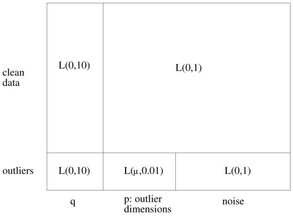
Data set design for simulation experiments. Observations are represented by rows and variables are represented by columns. For each instance, outliers comprise 10% of the data set.

7 Computational Results

L₁-PCA* is implemented and its performance on simulated and real-world data is compared to L₂-PCA, pcaPP, and L₁-PCA. The R package pcaPP is a publicly-available implementation of the L₁-norm-based PCA procedure developed by Croux and Ruiz-Gazen [8]. The approach implemented in pcaPP maximizes an L₁ measure of dispersion in the data to find successive locally-optimal directions of maximum dispersion. We implemented L₁-PCA, an algorithm developed by Ke and Kanade [17] that approximates L₁-norm best-fit subspaces directly which stands in contrast to the successive approaches L₁-PCA* and pcaPP.

L₁-PCA* is implemented in a C program that uses ILOG CPLEX 11.1 Callable Library [14] for the solution of the linear programs required for Step 3. The singular value decomposition in Step 5 is calculated using the function dgesvd in LAPACK [2]. The L₂-PCA and pcaPP implementations are publicly available in the stats [24] and pcaPP [11] packages for the R language for statistical computing [24]. The function used for L₂-PCA is prcomp. L₁-PCA is implemented as part of an R package that will be released at a later date [16]. All experiments are performed on machines with 2.6GHz Opteron processors and at least 4GB RAM.

Tests with simulated data

The implementations are tested on simulated data. Simulated data provide a controlled setting for comparison of data analysis algorithms and reveal trends that help make generalizable conclusions. The objectives for the data are to explore the impact of outliers on the procedures by varying the dimensionality and magnitude of outlier contamination. The data are generated such that a predetermined subspace contains most of the dispersion. The dimension of this “true” subspace is varied to assess the dependence on this data characteristic.

Each data set consists of n = 1000 observations with m dimensions. The first q dimensions define the predetermined subspace and the remaining dimensions contain noise. The first q dimensions are sampled from a Laplace(0, 10) distribution; the remaining dimensions are sampled from a Laplace(0, 1) distribution. Outliers are introduced in the data set by generating additional points where the first q dimensions are sampled from a Laplace(0, 10) distribution, the next p dimensions are sampled from a Laplace(μ, 0.01) distribution so that the outliers are on the same side of the true subspace, and the remaining m − p − q dimensions are sampled from a Laplace(0, 1) distribution. The problem suite also includes control data sets (p = 0, μ = 0) without outlier observations. Outlier observations comprise ten percent of each data set. We refer to the parameter p as the number of outlier-contaminated dimensions and the parameter μ as the outlier magnitude. Data sets are also generated by replacing distribution Laplace(0, 10) with N(0, 10), replacing Laplace(0, 1) with N(0, 1), and replacing Laplace(μ, 0.01) with N(μ, 0.01). Figure 3 is a schematic of the roles of the data components in the simulated data.

Tests are conducted for the configurations that result when m = 10, 100; q = 2, 5; p = 1, 2, 3; and μ = 25, 50, 75; in addition to the control data sets; for a total of 60 configurations. We define the error for an observation as the L₁ distance from its projected point in the best-fitting q-dimensional subspace determined by the four methods to the predetermined q-dimensional subspace.

The problem suite is processed by the L₁-PCA*, L₂-PCA, pcaPP, and L₁-PCA implementations. The results for Laplacian noise are reported in Tables 3-4 and the results for Gaussian noise are reported in Tables 5-6. These tables contain the mean and standard deviation of the sum of errors for 100 replications of each configuration.

Table 3.

Average (Standard Deviation) of L₁ Distance to True Subspace for m = 10 Laplacian Noise/Error 100 Replications for Each Configuration

q	p	μ	L1-PCA*	L2-PCA	pcaPP	L1-PCA
2	0	0	339.8 ( 66.0 )	329.1 ( 60.2 )	4600.2 ( 978.6 )	244.5 ( 46.2 )
2	1	25	328.5 ( 60.0 )	640.7 ( 185.9 )	5556.0 ( 1216.1 )	253.1 ( 48.7 )
2	2	25	371.5 ( 73.7 )	1515.7 ( 681.4 )	7456.1 ( 1711.5 )	253.9 ( 47.1 )
2	3	25	872.4 ( 427.8 )	8974.9 ( 3298.1 )	9145.1 ( 1852.6 )	5520.1 ( 4965.3 )
2	1	50	358.4 ( 75.6 )	6521.5 ( 393.8 )	8085.5 ( 1045.0 )	6211.4 ( 248.6 )
2	2	50	337.4 ( 60.4 )	11637.9 ( 111.2 )	10010.6 ( 1091.2 )	11611.9 ( 107.5 )
2	3	50	3644.8 ( 6662.5 )	16912.9 ( 80.8 )	11097.6 ( 1090.0 )	16850.1 ( 63.8 )
2	1	75	329.3 ( 61.8 )	8698.4 ( 88.5 )	8835.1 ( 940.1 )	8606.3 ( 58.0 )
2	2	75	16599.0 ( 75.1 )	16584.4 ( 71.7 )	9940.4 ( 1130.2 )	16538.7 ( 75.5 )
2	3	75	24372.2 ( 61.9 )	24371.8 ( 68.2 )	10288.8 ( 1297.9 )	24329.6 ( 56.6 )
5	0	0	347.5 ( 51.8 )	370.4 ( 56.0 )	4555.6 ( 716.1 )	273.3 ( 39.4 )
5	1	25	330.1 ( 50.2 )	884.1 ( 191.1 )	5819.6 ( 986.1 )	271.3 ( 40.9 )
5	2	25	386.3 ( 72.1 )	2503.5 ( 785.3 )	8258.3 ( 1549.5 )	286.0 ( 44.6 )
5	3	25	1644.9 ( 947.7 )	11485.5 ( 1308.1 )	10510.0 ( 1727.2 )	9581.7 ( 3963.4 )
5	1	50	395.5 ( 75.8 )	6447.3 ( 308.8 )	9985.7 ( 1142.8 )	6379.1 ( 269.2 )
5	2	50	326.1 ( 52.5 )	11636.4 ( 129.0 )	14075.7 ( 1017.2 )	11629.6 ( 110.4 )
5	3	50	3944.9 ( 6881.0 )	16882.8 ( 65.8 )	16555.9 ( 1136.5 )	16845.3 ( 78.1 )
5	1	75	325.3 ( 55.1 )	8719.7 ( 76.3 )	11983.1 ( 996.1 )	8659.6 ( 85.6 )
5	2	75	16554.3 ( 60.0 )	16584.5 ( 63.3 )	15153.7 ( 1198.3 )	16546.4 ( 67.5 )
5	3	75	24330.9 ( 64.1 )	24351.5 ( 56.6 )	16541.6 ( 1179.0 )	24327.3 ( 59.0 )

q: dimension of “true” underlying subspace

p: number of outlier-contaminated dimensions

μ: outlier magnitude

Table 4.

Average (Standard Deviation) of L₁ Distance to True Subspace for m = 100 Laplacian Noise/Error 100 Replications for Each Configuration

q	p	μ	L1-PCA*	L2-PCA	pcaPP	L1-PCA
2	0	0	5012.0 ( 294.1 )	4054.7 ( 223.0 )	42876.7 ( 2733.3 )	2965.2 ( 167.5 )
2	1	25	5079.1 ( 306.8 )	4379.2 ( 276.9 )	43127.7 ( 2088.2 )	2991.8 ( 164.3 )
2	2	25	5055.7 ( 272.7 )	5210.7 ( 754.1 )	45059.6 ( 2644.3 )	3001.6 ( 161.7 )
2	3	25	6069.4 ( 727.1 )	13567.6 ( 2811.4 )	46975.9 ( 2926.5 )	8774.4 ( 4563.1 )
2	1	50	5127.4 ( 295.5 )	9842.0 ( 500.7 )	46602.8 ( 2507.1 )	8628.0 ( 453.7 )
2	2	50	5052.1 ( 305.0 )	14850.5 ( 237.8 )	49793.2 ( 2478.7 )	13998.4 ( 339.3 )
2	3	50	6668.7 ( 4793.3 )	20106.7 ( 217.6 )	52352.1 ( 2922.9 )	19140.3 ( 144.6 )
2	1	75	5036.1 ( 260.9 )	11868.0 ( 213.0 )	49244.6 ( 2666.6 )	10923.4 ( 165.8 )
2	2	75	20649.4 ( 262.5 )	19790.3 ( 217.9 )	52503.2 ( 2703.2 )	18913.6 ( 155.2 )
2	3	75	28369.1 ( 262.8 )	27549.7 ( 211.9 )	54090.3 ( 3307.9 )	26720.3 ( 436.8 )
5	0	0	8590.3 ( 278.1 )	6933.6 ( 202.9 )	70283.2 ( 3071.5 )	5182.5 ( 187.5 )
5	1	25	8603.1 ( 285.1 )	7451.2 ( 326.7 )	71539.1 ( 3933.4 )	5178.2 ( 171.3 )
5	2	25	8663.4 ( 314.3 )	9014.1 ( 712.9 )	73553.8 ( 3275.1 )	5194.2 ( 213.9 )
5	3	25	10326.2 ( 922.5 )	18144.2 ( 1251.5 )	76066.9 ( 3690.2 )	15035.6 ( 2951.7 )
5	1	50	8682.2 ( 291.9 )	12879.5 ( 439.0 )	75432.8 ( 3286.9 )	11186.4 ( 420.0 )
5	2	50	8623.1 ( 306.7 )	18030.7 ( 251.3 )	82312.4 ( 3241.5 )	16459.9 ( 242.5 )
5	3	50	12340.6 ( 6879.0 )	23276.8 ( 257.7 )	86927.0 ( 4196.8 )	21677.5 ( 231.0 )
5	1	75	8564.1 ( 287.2 )	15107.4 ( 213.0 )	81899.0 ( 3897.0 )	13488.4 ( 192.7 )
5	2	75	24608.9 ( 292.8 )	22979.6 ( 216.2 )	87993.7 ( 3899.2 )	21373.5 ( 203.4 )
5	3	75	32371.0 ( 299.4 )	30743.9 ( 242.8 )	90029.9 ( 3800.5 )	29097.8 ( 194.9 )

q: dimension of “true” underlying subspace

p: number of outlier-contaminated dimensions

μ: outlier magnitude

Table 5.

Average (Standard Deviation) of L₁ Distance to True Subspace for m = 10 Gaussian Noise/Error 100 Replications for Each Configuration

q	p	μ	L1-PCA*	L2-PCA	pcaPP	L1-PCA
2	0	0	313.8 ( 61.6 )	253.1 ( 50.6 )	3312.2 ( 637.9 )	323.9 ( 64.9 )
2	1	25	342.2 ( 64.0 )	921.6 ( 408.7 )	4104.5 ( 870.0 )	323.4 ( 58.4 )
2	2	25	368.2 ( 75.4 )	6540.2 ( 373.4 )	5663.8 ( 1261.7 )	6675.4 ( 347.8 )
2	3	25	315.2 ( 56.2 )	9014.0 ( 161.8 )	7188.9 ( 1276.1 )	9019.2 ( 157.6 )
2	1	50	327.5 ( 66.1 )	5945.0 ( 60.8 )	6342.9 ( 923.5 )	5979.1 ( 68.3 )
2	2	50	4569.8 ( 5343.7 )	11188.4 ( 53.3 )	7725.0 ( 887.7 )	11262.7 ( 72.0 )
2	3	50	16428.7 ( 55.0 )	16400.3 ( 48.2 )	8622.2 ( 991.6 )	16433.2 ( 54.6 )
2	1	75	8464.7 ( 55.3 )	8420.7 ( 43.4 )	6804.2 ( 847.4 )	8470.5 ( 64.4 )
2	2	75	16217.4 ( 58.2 )	16181.2 ( 50.1 )	7650.8 ( 774.2 )	16230.9 ( 60.9 )
2	3	75	23914.2 ( 54.6 )	23886.2 ( 46.1 )	7743.1 ( 837.0 )	23923.6 ( 51.1 )
5	0	0	342.9 ( 43.3 )	272.7 ( 37.2 )	3323.9 ( 525.1 )	337.0 ( 46.9 )
5	1	25	378.1 ( 53.4 )	1381.1 ( 337.0 )	4747.7 ( 837.0 )	340.8 ( 51.2 )
5	2	25	416.6 ( 72.6 )	6544.6 ( 390.3 )	7142.7 ( 1021.1 )	6751.3 ( 402.9 )
5	3	25	309.7 ( 48.3 )	8961.2 ( 166.0 )	9876.1 ( 1164.5 )	9023.1 ( 155.9 )
5	1	50	340.6 ( 56.7 )	5963.8 ( 59.9 )	8629.7 ( 645.3 )	6030.6 ( 79.1 )
5	2	50	10909.0 ( 1875.4 )	11189.1 ( 46.9 )	11456.6 ( 699.8 )	11262.6 ( 58.8 )
5	3	50	16383.4 ( 49.1 )	16357.3 ( 37.6 )	12814.8 ( 705.6 )	16392.5 ( 53.4 )
5	1	75	8495.9 ( 48.2 )	8438.6 ( 40.6 )	9399.0 ( 755.7 )	8501.7 ( 52.6 )
5	2	75	16221.3 ( 49.0 )	16178.6 ( 39.4 )	11348.0 ( 1056.0 )	16229.8 ( 47.0 )
5	3	75	23878.3 ( 38.5 )	23854.2 ( 37.3 )	11995.8 ( 871.1 )	23884.5 ( 45.6 )

q: dimension of “true” underlying subspace

p: number of outlier-contaminated dimensions

μ: outlier magnitude

Table 6.

Average (Standard Deviation) of L₁ Distance to True Subspace for m = 100 Gaussian Noise/Error 100 Replications for Each Configuration

q	p	μ	Li-PCA*	L2-PCA	pcaPP	L1-PCA
2	0	0	3941.4 ( 242.1 )	3130.7 ( 171.0 )	30524.2 ( 1520.4 )	3873.4 ( 222.0 )
2	1	25	3995.1 ( 221.7 )	3841.3 ( 404.3 )	31296.6 ( 1782.1 )	3919.1 ( 205.5 )
2	2	25	4007.9 ( 236.1 )	8910.4 ( 421.6 )	33394.3 ( 2204.3 )	9657.8 ( 342.9 )
2	3	25	3969.2 ( 229.6 )	11418.2 ( 228.3 )	35798.6 ( 2353.9 )	11982.3 ( 244.1 )
2	1	50	3948.1 ( 208.7 )	8348.5 ( 145.6 )	35591.2 ( 2142.0 )	8964.0 ( 184.5 )
2	2	50	7585.4 ( 4947.6 )	13599.2 ( 155.6 )	38132.4 ( 2254.6 )	14294.2 ( 174.5 )
2	3	50	19447.2 ( 190.7 )	18787.3 ( 148.9 )	39397.2 ( 2142.2 )	19504.4 ( 545.8 )
2	1	75	11435.0 ( 780.0 )	10826.2 ( 144.5 )	37157.3 ( 2191.3 )	11465.6 ( 209.1 )
2	2	75	19260.1 ( 197.1 )	18565.4 ( 135.0 )	39185.0 ( 2395.3 )	19254.7 ( 202.4 )
2	3	75	26936.7 ( 169.2 )	26268.0 ( 149.6 )	39902.9 ( 2575.0 )	26891.1 ( 178.7 )
5	0	0	6513.4 ( 215.0 )	5153.2 ( 184.8 )	49849.0 ( 3663.3 )	6399.8 ( 215.9 )
5	1	25	6556.8 ( 224.8 )	6252.6 ( 417.5 )	51223.5 ( 5684.2 )	6408.6 ( 208.2 )
5	2	25	6624.2 ( 247.0 )	11230.7 ( 358.5 )	54312.2 ( 3270.9 )	12712.2 ( 399.8 )
5	3	25	6474.8 ( 197.4 )	13683.9 ( 217.7 )	57664.4 ( 3355.7 )	14944.9 ( 270.4 )
5	1	50	6465.6 ( 240.3 )	10696.2 ( 188.0 )	58066.3 ( 2745.5 )	11983.2 ( 310.2 )
5	2	50	16971.2 ( 1523.5 )	15931.6 ( 159.6 )	63716.0 ( 2714.6 )	17261.5 ( 201.8 )
5	3	50	22360.3 ( 227.1 )	21095.7 ( 161.0 )	66299.2 ( 2812.8 )	22370.1 ( 231.8 )
5	1	75	14467.8 ( 219.5 )	13184.2 ( 174.3 )	61481.8 ( 3534.9 )	14444.7 ( 259.4 )
5	2	75	22192.6 ( 233.2 )	20917.8 ( 174.6 )	65874.3 ( 3126.6 )	22254.4 ( 316.3 )
5	3	75	29864.4 ( 226.1 )	28586.3 ( 177.4 )	67072.6 ( 2599.8 )	29877.5 ( 226.1 )

q: dimension of “true” underlying subspace

p: number of outlier-contaminated dimensions

μ: outlier magnitude

Our experiments include eight controls (m = 10, 100, q = 2, 5, Laplacian and Gaussian noise) when μ = 0 and p = 0 for each distribution of noise. In these data sets, there are no outliers. L₂-PCA outperforms L₁-PCA* in seven of the eight control experiments. As expected, L₂-PCA outperforms L₁-PCA* in the control experiments when the noise is Gaussian. In the presence of Laplacian noise, L₁-PCA* performs better than L₂-PCA when the dimension of the underlying subspace is higher (q = 5) and the dimension of the original data is lower (m = 10). The explanation is that the fitted subspaces of successively smaller dimension derived by L₁-PCA* are optimal with respect to the projected data at each iteration and do not necessarily coincide with the L₁ best-fit subspace with respect to the original data points. Therefore, there is a degradation in the performance of L₁-PCA* as the dimension of the true subspace decreases. L₁-PCA approximates subspaces directly, and performs best in the control experiments in the presence of Laplacian noise. For the control experiments, pcaPP is not competitive.

Figure 4 illustrates the results for q = 5 and Laplacian noise. The figure compares the performance of the four implementations with respect to outlier magnitude μ, number of outlier-contaminated dimensions p, and number of total dimensions m. For small contamination (μ = 25 and p = 1), there is little discernible difference among L₁-PCA*, L₁-PCA, and L₂-PCA, and these three methods outperform pcaPP. For moderate levels of contamination (μ = 50), L₁-PCA* provides a clear advantage in the presence of outliers. The other methods fit the outlier observations, while L₁-PCA* ignores them and fits the clean data. In the cases with extreme outlier contamination (μ = 75 and p ≥ 2), all of the methods break down and fit the outlier observations with the exception of pcaPP when m = 10, μ = 75, and p = 3. This advantage for pcaPP for μ = 75 and p = 3 is not present when m = 100. This adverse reaction of pcaPP to an increase in dimension can be explained by a dimensionality curse effect since the algorithm relies on a grid search procedure. Similar patterns are observed in the experiments when the noise are Gaussian, except that the increased noise in the data causes each method to break down sooner (Figure 5).

Figure 4.

Laplacian noise. The sum of errors, the sum of L₁ distances of projected points in a 5-dimensional subspace to the “true” 5-dimensional subspace of the data, versus outlier magnitude with Laplacian noise, for dimensions m = 10 and m = 100, and p = 1, 2, 3. The average sum of errors over 100 iterations is plotted. Error bars represent one standard deviation. The parameter p is the number of outlier-contaminated dimensions.

Figure 5.

Gaussian noise. The sum of errors, the sum of L₁ distances of projected points in a 5-dimensional subspace to the “true” 5-dimensional subspace of the data, versus outlier magnitude with Gaussian noise, for dimensions m = 10 and m = 100, and p = 1, 2, 3. The average sum of errors over 100 iterations is plotted. Error bars represent one standard deviation. The parameter p is the number of outlier-contaminated dimensions.

For each method, as μ and p are increased, the breakdown point is reached where the methods begin to fit the outlier observations better than the non-contaminated data. For Laplacian noise and for p = 1, 2, 3, L₁-PCA* does not break down, even as μ is increased to 50, while significant increases in the sum of errors are seen for L₂-PCA, pcaPP, and L₁-PCA. The approach of the breakdown point for L₁-PCA* and L₂-PCA as p and μ increase is signaled in Tables 3-6 by an increase in the standard deviations of the sum of errors. For the configurations with large standard deviations; such as m = 10, q = 2, p = 3, and μ = 50 for L₁-PCA*; the methods fit the non-contaminated data for some samples and fit the outlier observations for other samples which result in drastically different sums of errors. The standard deviations of the sums of errors for pcaPP are larger than those for the other methods for almost every configuration, an indication that pcaPP is sensitive to small changes in the data. For q = 5 and Laplacian noise, we can see in Figure 4 that L₁-PCA* is less susceptible to breakdown and only breaks down when p ≥ 2 and μ = 75. In summary, L₁-PCA* is competitive with other methods in the presence of low outlier contamination and provides substantial benefits in the presence of moderate outlier contamination. Our experiments show that L₁-PCA* is the indicated procedure in the presence of unbalanced outlier contamination. These experiments validate the intuition that L₁-PCA* is robust to outliers because of the underlying reliance on optimally-fitted L₁ subspaces.

Tests with Real Data

The four implementations; L₁-PCA*, L₂-PCA, pcaPP, and L₁-PCA; are applied to real-world data that are known to contain outliers. The “Milk” data set is introduced by Daudin [9] and used by Choulakian [7] for tests with an L₁ projection-pursuit algorithm for PCA. The “McDonald and Schwing” data set is introduced by McDonald and Schwing [23] and is used by Croux and Ruiz-Gazen [8] for tests with an L₁ projection-pursuit algorithm for PCA. For each data set, the data are centered by subtracting the attribute medians.

Figure 6 contains plots of the sum of residuals of non-outlier observations against the dimension of the fitted subspace for the two data sets. The residual for an observation is measured as the L₁ distance from the original point to the projected point in the fitted subspace. If a method is properly ignoring the outlier observations and fitting the non-contaminated data, then the plotted values should be small.

Figure 6.

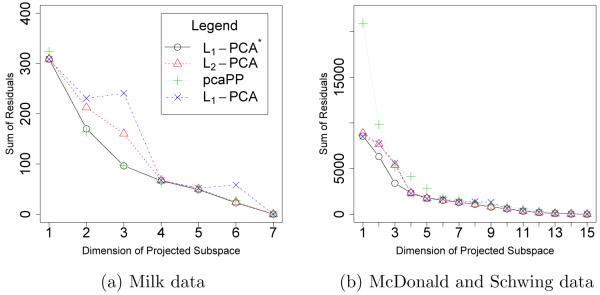
Sum of residuals of non-outlier observations versus the dimension of the fitted subspace for (a) the Milk data set and (b) the McDonald and Schwing data set.

Figure 6(a) contains the results for the Milk data set. Observations 17, 47, and 70 are identified as outliers in previous analyses (see [7]). When the outliers are removed the correlation of variables 4 and 6, 4 and 7, 5 and 6, and 5 and 7 increase by more than 0.3 each when outliers are removed, indicating that the outlier contamination is present in more than one dimension. The sum of residuals for the non-outlier observations for L₁-PCA* and pcaPP are almost identical and are less than that for L₂-PCA and L₁-PCA for two and three dimensions.

The residuals for the non-outliers in the McDonald and Schwing data set are depicted in Figure 6(b). Observations 29 and 48 are identified as outliers in previous analyses (see [8]). When the outliers are removed, the correlation of variables 5 and 12, 5 and 13, 12 and 15, 13 and 14, 13 and 16 increase by at least 0.3 each, indicating that the outlier contamination is present in more than one dimension. The sum of residuals for non-outlier observations for pcaPP is larger for smaller-dimensional fitted subspaces when compared to L₁-PCA*, L₂-PCA, and L₁-PCA. Procedure pcaPP appears to be pushing the fitted subspace away from the outlier observations at the expense of the fit of non-outlier observations.

The expectation that L₁-PCA* performs well in the presence of outliers is validated for these data sets. For the two real data sets, Figure 6 shows that L₁-PCA* generates subspaces that are competitive in terms of having low residuals for non-outliers. The diminished advantage of using L₁-PCA* for these real data sets when compared to the simulated data can be attributed to the fact that the outliers in the real data are more balanced in that they are not located on one side of the best-fitting subspace for the non-contaminated data. Real data with outlier contamination are likely to have some imbalance in the location of the outliers. L₁-PCA* is well-suited in these situations.

8 Conclusions

This paper proposes a new procedure for PCA based on finding successive L₁-norm best-fit sub-spaces. The result is a pure L₁ PCA procedure in the sense that it uses the globally optimal solution of an optimization problem where the sum of L₁ distances is minimized. Several “pure” L₁ PCAs are possible by taking any one of the properties of traditional L₂ PCA and using the L₁ norm. We describe a complete PCA procedure, L₁-PCA*, based on this result, and include formulas for correspondences with familiar L₂-PCA outputs. The procedure is tested on simulated and real data. The results for simulated data indicate that the procedure can be more robust than L₂-PCA and competing L₁-based procedures, pcaPP and L₁-PCA, for unbalanced outlier contamination and for a wide range of outlier magnitudes. Experiments with real data confirm that L₁-PCA* is competitive in data sets with outliers. L₁-PCA* represents an alternative tool for the numerous applications of PCA.

Figure 7.

Laplacian noise. The sum of errors, the sum of L₁ distances of projected points in a 2-dimensional subspace to the “true” 2-dimensional subspace of the data, versus outlier magnitude with Laplacian noise, for dimensions m = 10 and m = 100, and p = 1, 2, 3. The average sum of errors over 100 iterations is plotted. Error bars represent one standard deviation. The parameter p is the number of outlier-contaminated dimensions.

Figure 8.

Gaussian noise. The sum of errors, the sum of L₁ distances of projected points in a 2-dimensional subspace to the “true” 2-dimensional subspace of the data, versus outlier magnitude with Gaussian noise, for dimensions m = 10 and m = 100, and p = 1, 2, 3. The average sum of errors over 100 iterations is plotted. Error bars represent one standard deviation. The parameter p is the number of outlier-contaminated dimensions.

References

- [1].Agarwal S, Chandraker MK, Kahl F, Kriegman D, Belongie S. Practical global optimization for multiview geometry. Lecture Notes in Computer Science. 2006;3951:592–605. [Google Scholar]
- [2].Anderson E, Bai Z, Bischof C, Blackford S, Demmel J, Dongarra J, Du Croz J, Greenbaum A, Hammarling S, McKenney A, Sorensen D. LAPACK Users’ Guide. third edition Society for Industrial and Applied Mathematics; Philadelpha, PA: 1999. [Google Scholar]
- [3].Appa G, Smith C. On L1 and Chebyshev estimation. Mathematical Programming. 1973;5:73–87. [Google Scholar]
- [4].Baccini A, Besse P, de Faguerolles A. A L1-norm PCA and heuristic approach; Proceedings of the International Conference on Ordinal and Symbolic Data Analysis; 1996.pp. 359–368. [Google Scholar]
- [5].Brooks JP, Dulá JH. The L1-norm best-fit hyperplane problem. Applied Mathematics Letters. doi: 10.1016/j.aml.2012.03.031. in press, accepted March 2012. [DOI] [PMC free article] [PubMed] [Google Scholar]
- [6].Charnes A, Cooper WW, Ferguson RO. Optimal estimation of executive compensation by linear programming. Management Science. 1955;1:138–150. [Google Scholar]
- [7].Choulakian V. L1-norm projection pursuit principal component analysis. Computational Statistics and Data Analysis. 2006;50:1441–1451. [Google Scholar]
- [8].Croux C, Ruiz-Gazen A. High breakdown estimators for prinicpal components: the projection-pursuit approach revisited. Journal of Multivariate Analysis. 2005;95:206–226. [Google Scholar]
- [9].Daudin JJ, Duby C, Trecourt P. Stability of principal component analysis studied by the bootstrap method. Statistics. 1988;19:241–258. [Google Scholar]
- [10].Ding C, Zhou D, He X, Zha H. R1-pca: Rotational invariant L1-norm principal component analysis for robust subspace factorization; Proceedings of the 23rd International Conference on Machine Learning; 2006.pp. 281–288. [Google Scholar]
- [11].Filzmozer P, Fritz H, Kalcher K. pcaPP: Robust PCA by projection pursuit. 2009 [Google Scholar]
- [12].Galpin JS, Hawkins DM. Methods of L1 estimation of a covariance matrix. Computational Statistics and Data Analysis. 1987;5:305–319. [Google Scholar]
- [13].Gao J. Robust L1 principal component analysis and its Bayesian variational inference. Neural Computation. 2008;20:555–572. doi: 10.1162/neco.2007.11-06-397. [DOI] [PubMed] [Google Scholar]
- [14].ILOG . ILOG CPLEX Division. 889 Alder Avenue, Incline Village, Nevada: 2009. [Google Scholar]
- [15].Jollie IT. Principal Component Analysis. 2nd edition Springer; 2002. [Google Scholar]
- [16].Jot S. pcaL1: An R package of principal component analysis methods using the L1 norm. Master’s thesis, Statistical Sciences and Operations Research, Virginia Commonwealth University; Richmond, Virgina: 2011. [Google Scholar]
- [17].Ke Q, Kanade T. Robust subspace computation using L1 norm. Technical Report CMU-CS-03-172, Carnegie Mellon University; Pittsburgh, PA: 2003. [Google Scholar]
- [18].Kier LB, Seybold PG, Cheng C-K. Cellular automata modeling of chemical systems: a textbook and laboratory manual. Springer; 2005. [Google Scholar]
- [19].Kwak N. Principal component analysis based on L1-norm maximization. IEEE Transactions on Pattern Analysis and Machine Intelligence. 2008;30:1672–1680. doi: 10.1109/TPAMI.2008.114. [DOI] [PubMed] [Google Scholar]
- [20].Li G, Chen Z. Projection-pursuit approach to robust distpersion matrices and principal components: Primary theory and Monte Carlo. Journal of the American Statistical Association. 1985;80:759–766. [Google Scholar]
- [21].Mangasarian OL. Arbitrary-norm separating plane. Operations Research Letters. 1999;24:15–23. [Google Scholar]
- [22].Martini H, Schöbel A. Median hyperplanes in normed spaces - a survey. Discrete Applied Mathematics. 1998;89:181–195. [Google Scholar]
- [23].McDonald GC, Schwing RC. Instabilities of regression estimates relating air pollution to mortality. Technometrics. 1973;15:463–481. [Google Scholar]
- [24].R Development Core Team . R: A Language and Environment for Statistical Computing. R Foundation for Statistical Computing; Vienna, Austria: 2008. ISBN 3-900051-07-0. [Google Scholar]
- [25].Sp̈ath H, Watson GA. On orthogonal linear l1 approximation. Numerische Mathematik. 1987;51:531–543. [Google Scholar]
- [26].Wagner HM. Linear programming techniques for regression analysis. Journal of the American Statistical Association. 1959;54:206–212. [Google Scholar]
Associated Data
This section collects any data citations, data availability statements, or supplementary materials included in this article.