Nonlinear, Multilevel Mixed-Effects Approach for Modeling Longitudinal Standard Automated Perimetry Data in Glaucoma

Abstract

Purpose.

Ordinary least squares linear regression (OLSLR) analyses are inappropriate for performing trend analysis on repeatedly measured longitudinal data. This study examines multilevel linear mixed-effects (LME) and nonlinear mixed-effects (NLME) methods to model longitudinally collected perimetry data and determines whether NLME methods provide significant improvements over LME methods and OLSLR.

Methods.

Models of LME and NLME (exponential, whereby the rate of change in sensitivity worsens over time) were examined with two levels of nesting (subject and eye within subject) to predict the mean deviation. Models were compared using analysis of variance or Akaike's information criterion and Bayesian information criterion, as appropriate.

Results.

Nonlinear (exponential) models provided significantly better fits than linear models (P < 0.0001). Nonlinear fits markedly improved the validity of the model, as evidenced by the lack of significant autocorrelation, residuals that are closer to being normally distributed, and improved homogeneity. From the fitted exponential model, the rate of glaucomatous progression for an average subject of age 70 years was −0.07 decibels (dB) per year. Ten years later, the same eye would be deteriorating at −0.12 dB/y.

Conclusions.

Multilevel mixed-effects models provide better fits to the test data than OLSLR by accounting for group effects and/or within-group correlation. However, the fitted LME model poorly tracks visual field (VF) change over time. An exponential model provides a significant improvement over linear models and more accurately tracks VF change over time in this cohort.

OLS methods are inappropriate for performing trend analyses on repeatedly measured longitudinal data. Instead, a nonlinear (exponential) model provides a significant improvement over linear models and more accurately tracks visual field change over time in this cohort.

Introduction

Glaucoma, characterized by a progressive optic neuropathy and damage to the visual field (VF), is a leading cause of irreversible blindness worldwide.^1,2 Of vital interest in glaucoma management is the assessment of disease progression by monitoring functional and structural changes.^3–5 Although both functional and structural changes can provide evidence of disease progression, tracking glaucomatous VF progression is of key importance because functional testing directly relates to the activities of daily living.⁶ Standard automated perimetry, for example as performed by the Humphrey Field Analyzer (Carl Zeiss Meditec Inc., Dublin, CA), is currently the most widely used test for detecting functional damage.

In recent decades, numerous analyses have been developed for detecting VF damage and for monitoring its progression over time such as Glaucoma Progression Analysis and PROGRESSOR.⁷ Trend analyses are increasingly being performed on perimetry data gathered from patients with glaucoma. Some examples are trend analyses of the mean deviation (MD), the Visual Field Index, or pointwise linear regression of VF sensitivities. Despite the availability of various advanced technologies for tracking functional progression, trend analyses using ordinary least squares linear regression (OLSLR) are still widely used statistical methods in the vision science literature^8–12 because of its straightforward and mathematically more tractable applications. Numerous studies have used clinical applications of OLS regression analyses, for example when measuring treatment effects,¹¹ examining characteristics of types of glaucoma,¹² and assessing the rate of VF progression.¹⁰ However, OLSLR, the most commonly used method for trend analysis in the literature, may be inappropriate for modeling longitudinal data. Its validity, and hence the P values it produces, relies on not violating several assumptions, as discussed below.

First, one of the fundamental assumptions underlying the OLS approach is that the residuals have homogeneous variance. However, various studies^13–15 have suggested that the variability of VF sensitivities is increased when sensitivity is lower in both normal and damaged eyes.^13,15 Therefore, performing an OLSLR on longitudinally collected data violates the principle of homoscedasticity.

A second assumption within the OLS framework is that the residuals (the differences between the observed values and those predicted by the trend over time) are uncorrelated. In longitudinal data, it is common for temporal autocorrelation to be present even if no glaucomatous progression is observed.¹⁶ This can be caused by longer-term random fluctuations, whose effects last more than the interval between tests, or by longer-term fluctuations in causative factors that were not included in the model. The same effect can also occur when a linear fit is imposed on data that are actually changing in a nonlinear manner. As an example, the measure of interest (in this case, the MD) is assumed to change at a constant rate over time. Recent cross-sectional studies^17–19 indicate that change in sensitivity when expressed on a linear (1/contrast) scale appears to be proportional to the percentage loss of retinal ganglion cells (RGCs). Therefore, given the logarithmic nature of the decibel (dB) scale used in perimetry, linear change in sensitivity over time implies that the proportion of remaining RGCs that die each year must remain constant. That is, if 10% of the RGCs die in a year, 10% of the surviving RGCs would die in the following year, and so forth. If we hypothesize an alternative formulation, where the actual number of remaining RGCs that die each year remains constant, resulting in a linear decline in structural measures such as retinal nerve fiber layer thickness, then based on the cross-sectional findings this would result in the loss of sensitivity in decibels appearing to accelerate exponentially. If a linear fit is placed over data that are accelerating downward exponentially, the residuals will tend to be positive in the center of the period and negative at either end of the sequence, causing potentially significant temporal autocorrelation. In the presence of heteroscedasticity or temporal autocorrelation, OLS estimators are no longer the best linear unbiased estimators. Thus, statistics and confidence intervals from OLS may not be valid for drawing inference.

Third, longitudinally collected data are often grouped by one or more grouping factors. In the case of ophthalmic tests, data are grouped within an eye (i.e., ≥50 VF locations per eye), and eyes are grouped in pairs for each individual. Observations taken within the same eye or from the same individual are likely to be more similar than observations taken from a different eye or person. When OLSLR is performed on grouped data, residuals from the same group (e.g., two eyes of an individual or VF locations within an eye) tend to have the same sign, either positive or negative. This indicates the need for more sophisticated methods that take into account correlation among observations within the same group.

In this study, we use multilevel mixed-effects methods that account for group effects (both within eyes and between fellow eyes of the same individual), as well as temporal autocorrelation of within-group errors, to generate more valid P values for assessing the significance of change in VF sequences from participants with glaucoma. These findings are also compared with those from OLSLR. We then consider the use of a nonlinear model in which VF sensitivity declines exponentially with time based on the alternative formulation outlined above, and we determine whether this removes evidence of autocorrelation. We demonstrate and test these statistical methods with a relatively simple predictive model using only age as a predictor of the rate of glaucomatous field change. However, the overall goal of this work is to aid in the development of better predictive models that will help clinicians manage patients with glaucoma.

Methods

Data

Data from participants with suspected or early glaucoma or with high-risk ocular hypertension from the ongoing Portland Progression Project at Devers Eye Institute were used in this study. The study protocol was approved by the Legacy Health Institutional Review Board. This study complies with the Health Insurance Portability and Accountability Act of 1996 and is in agreement with the provisions of the Declaration of Helsinki. Consent was obtained from all participants after they were well informed about the risks and benefits of participation.

Initially, participants were tested annually with various functional and structural tests. In 2009, testing was switched to 6-month intervals for all participants. At baseline, participants either had early glaucoma (standard automated perimetry MD no worse than −6 dB) or had ocular hypertension (untreated intraocular pressure repeatedly >22 mm Hg) plus one or more risk factors for developing glaucoma as determined by their eye care provider. Risk factors included age older than 70 years,^5,20 African ancestry,²⁰ systemic hypertension,²¹ peripheral vasospasm,²² migraine,²³ self-reported family history of glaucoma,²⁴ disc hemorrhage,^25,26 diet-controlled diabetes,²⁷ and/or previously diagnosed glaucomatous optic neuropathy or suspicious optic nerve head appearance (cup-disc ratio asymmetry > 0.2) and neuroretinal rim notching or narrowing. Participants having visual acuity worse than 20/40 in either eye or worse than mild glaucoma, cataract, or media change at baseline were excluded. Other exclusion criteria included any other disease or the use of any medications likely to affect the VF or having undergone intraocular surgery (except for uncomplicated cataract surgery).

Standard automated perimetry VF testing was performed using a Humphrey Field Analyzer II (Carl Zeiss Meditec Inc.).²⁸ Initially, we used the Full Threshold algorithm and the 30-2 test pattern but later used the 24-2 test pattern and the Swedish Interactive Threshold Algorithm (SITA).²⁹ All MD values used in this study were 24-2 equivalent. This was accomplished by including earlier 30-2 tests within a Guided Progression Analysis³⁰ sequence that included at least one 24-2 test. The Humphrey Field Analyzer II (Carl Zeiss Meditec Inc.) then produces 24-2 equivalent MDs for the included 30-2 tests. Previously, we have shown that there is no difference in MD values generated by the Full Threshold and SITA Standard algorithms,³¹ so there is no concern with using data from both. An optimal lens correction was placed before the tested eye, and an eye patch was used to occlude the fellow eye. All subjects had previous experience with VF testing before entering the study, and most had undergone multiple previous tests. Tests with greater than 33% fixation losses or false negatives or with greater than 15% false positives were considered unreliable and were excluded.

Statistical Analysis

All statistical analyses were performed using statistical computing software R.³² Only participants with 10 or more observations per eye meeting the reliability criteria were included in the analyses. Follow-up time and age at the time of testing centered to its mean (a suggested risk factor for glaucomatous progression²⁰) were used as covariates. To find the best predictive model for the MD, both linear mixed-effects (LME) and nonlinear mixed-effects (NLME) models with two levels of nesting (subject and eye within subject) were fitted (details of the models considered are given in the Appendix). Discrete and continuous autoregressive methods were tested to examine temporal dependency likely to be present in within-group errors. Autoregressive (discrete or continuous) methods (CAR1) are used to model serial correlation of within-group errors in time series and longitudinal data, where the correlation between residuals from the model decreases exponentially with the time difference between measurements.³³

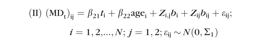
Therefore, four mixed-effects models were compared. As detailed in the Appendix, these include the following: (1) model I (linear progression over time, uncorrelated residuals), (2) model II (linear progression over time, autocorrelated residuals), (3) model III (nonlinear [exponential] progression over time, uncorrelated residuals), and (4) model IV (nonlinear progression over time, autocorrelated residuals).

The goodness of fit of models was compared using analysis of variance (ANOVA) or Akaike's information criterion (AIC) and Bayesian information criterion (BIC), as appropriate. Nested models (models I vs. II and models III vs. IV) are compared based on P values from ANOVA. Nonnested models (models I vs. III and models II vs. IV) cannot be compared using ANOVA and so instead are compared based on AIC and BIC, with smaller AIC and BIC indicating a better fit to the data. These AIC (2θ − 2log(L)) and BIC (θlog(L) − 2log(L)) are commonly used penalized model selection criteria for comparison and selection of models, where θ, L, and n are the total number of parameters to be estimated, the likelihood function, and the sample size, respectively. θ acts to penalize models with a greater number of free parameters.

Results

In total, 4179 VFs from 271 eyes of 138 participants were used. At baseline, the mean age was 56.86 (±SD 10.38) years, the MD was −0.02 (±2.09) dB, and 11% of participants had an MD of −2 dB or less. The average number of VF tests for each eye was 16. The average follow-up duration was 7.22 (±4.33) years.

Figure 1 shows the box plots of residuals from the OLSLR fit (displaying only a small sample of the subjects for better visualization), together with an autocorrelation plot of the residuals for a subject. These plots indicate the problem of using OLSLR on longitudinally collected data. Significant autocorrelation is evident, as indicated by the vertical lines (Fig. 1a) falling outside the normal limits for uncorrelated data (horizontal dashed lines). This violates the fundamental assumption of independence that underlies the OLS method. Furthermore, residuals from the same eyes and/or subject from OLSLR fits are not centered at zero (Fig. 1b), indicating that a mixed-effects model is needed to incorporate group effects.

Figure 1. .

Empirical autocorrelation plots (a) and residuals for a sample of subjects (b) from the OLSLR fit.

Table 1 and Table 2 give goodness-of-fit values for the candidate models and P values from ANOVA comparisons, respectively. Model II provides a significantly better fit than model I (P < 0.0001), indicating the presence of significant temporal autocorrelation that needs to be taken into account when performing linear fits. The AIC and BIC are much lower (better) for model III and model IV compared with any of the candidate LME models (Table 1) and show that exponential models fit sequences of MD values significantly better than assuming linear change over time. However, model III and model IV provide equivalent fits (P = 0.47). This indicates that when a suitable nonlinear model is used to examine change over time temporal autocorrelation is no longer significant. It appears to be caused by incorrectly imposing a linear fit, rather than by long-term fluctuation acting within the sequences.

Table 1. .

AIC and BIC Comparison of Various Candidate Mixed-Effects Models

Model	AIC	BIC
I	12,850.03	12,913.41
II	12,742.35	12,812.07
III	12,259.04	12,322.42
IV	12,261.55	12,331.28

Model I is a two-level LME with independent within-group error. Model II is a two-level LME model with continuous within-group temporal correlation structure (CAR1). Model III is a two-level NLME with independent within-group error. Model IV is a two-level NLME with continuous within-group temporal correlation structure.

Table 2. .

ANOVA Comparison of Candidate Mixed-Effects Models

Model	II	III	IV
I	P < 0.0001	NA*	P < 0.0001
II		P < 0.0001	NA*
III			P = 0.47

^Pvalues are from an ANOVA comparison between the two models indicated. The models are defined in Table 1.

^*Not available for nonnested models.

Significant autocorrelation between longitudinal data is detected in the plot of standardized residuals from the two-level LME model (Fig. 2), as indicated by the vertical lines extending beyond the limits that would be expected in the absence of autocorrelation (dashed horizontal lines). We examined the within-group correlation structure using both a discrete (AR) and continuous (CAR1) autoregressive structure. Because of the regularity of testing in this data set, there was very little difference (approximately equivalent AIC and BIC), but the continuous autoregressive structure is more practical and generalizable because it can be used directly in data sets with less regular temporal sampling.

Figure 2. .

Empirical autocorrelation plots of the residuals from LME model I.

Figure 3 shows diagnostic plots for model II. Errors from model II are now closer to being uncorrelated (Fig. 3a). However, the plot of standardized residuals versus the fitted values from model II indicates that the variance of the residuals increases as the fitted MD value decreases (Fig. 3b), violating the assumptions of constant within-group error variance. The fact that variability goes up with damage, as we have seen here, is consistent with the findings from previous studies.^13–15,34

Figure 3. .

Empirical autocorrelation plots (a) and a scatter plot of the standardized residuals versus fitted values (b) from model II.

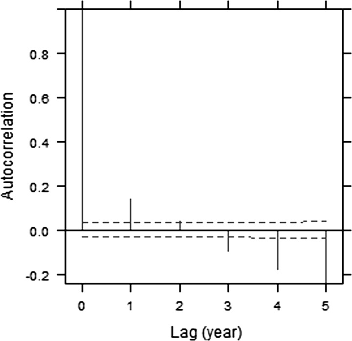
Figure 4 shows similar diagnostic plots of model III. The plot of standardized residuals versus the fitted values (Fig. 4b) indicates that residuals are symmetrically distributed around zero, with improved homogeneity compared with model II. In addition, no significant autocorrelation is observed up to 2 years on the empirical autocorrelation plots (Fig. 4a). The negative autocorrelation in the plot with higher lags is less reliable because estimates of autocorrelation for greater intervals are based on fewer residual pairs.²² This apparent lack of autocorrelation is consistent with the fact that when using NLME models there is no longer a significant benefit in accounting for correlated errors (models III vs. IV, P = 0.47). This supports our earlier assertion that errors could appear correlated if a linear fit is imposed onto nonlinear data.

Figure 4. .

Empirical autocorrelation plots (a) and a scatter plot of the standardized residuals versus fitted values (b) from model III.

Table 3 gives population estimates of the model parameters (λ₀, κ₀, and γ₀), corresponding SEs, and associated P values for the exponential model III. The average baseline MD (λ₀) and intercept of rate (κ₀) are significantly different from zero (P < 0.0001). The estimated maximum correlation among the fitted parameters was −0.2, indicating no overfitting. The predicted sensitivity for an average subject at time (t) is given by MD_t = λ₀ − exp(κ₀ + γ₀ · age)t, with the rate of change given by −(κ₀ + γ₀ · age) · exp(κ₀ + γ₀ · age)t. For an average 70-year-old subject in this cohort (i.e., when the random effects are set to be zero), his or her MD at time zero (i.e., baseline) is 0.26 dB, with a rate of change of −0.062 dB/y. Ten years later (i.e., t = 10), the VF will be deteriorating at −0.11 dB/y.

Table 3. .

Estimates of Fixed-Effects Parameters for NLME Model III

Parameter	Estimate (SE)	P Value
λ0, dB	1.26 (0.15)	<0.0001
κ0, dB/y	0.064 (0.008)	<0.0001
γ0, dB/y	−0.0009 (0.0006)	0.17

Figure 5 shows the augmented predictions to assess the adequacy of the fitted exponential model III (shown only for a few candidate subjects representing different cases). It is evident that the exponential model III is in close agreement with the observed MDs. The adequacy of the exponential model for fitting and predicting test data is apparent.

Figure 5. .

Within-group predictions (line) and observed MD (circles) versus time using the exponential model III for four subjects in the study.

Discussion

Accurate monitoring of glaucomatous progression is essential for better patient management. Such progression is often examined by performing OLSLR. Our study shows that tracking VF progression using OLSLR is insufficient for longitudinal data. Ordinary least squares linear regression ignores the grouping structure and heteroscedasticity of longitudinally collected ophthalmic data. In addition, errors from OLSLR are correlated. As a consequence, OLS methods overestimate the significance of trends, giving potentially inaccurate information about disease progression and its risk factors. For example, age is a highly significant predictor (P < 0.0001) when the MD is fitted using OLSLR. However, age is not a significant risk factor (P > 0.05) using either the fitted LME or NLME models. Note that this does not imply that age is not in fact associated with progression because the power to detect an effect may not be sufficient in this data set. Lack of evidence of an effect should not be taken as evidence for the lack of an effect. However, it illustrates that the significance of an effect can be overstated when an inappropriate model is used.

Unlike OLSLR, LME methods adequately incorporate group effects and within-group correlation and provide improvement over OLSLR. However, our results show that this linear formulation is still suboptimal for monitoring functional change over time. A nonlinear fit, whereby sensitivity declines exponentially on a decibel scale, markedly improved the validity of the model, as evidenced by the lack of significant autocorrelation, residuals that are closer to being normally distributed, and improved homogeneity.

The use of an exponential model is well supported by recent work on the structure-function relationship. It is consistent with a constant rate of RGC loss, without requiring the existence of a functional reserve.³⁵ The often-reported delay between when structural loss is first detected and when functional loss is first reported could be partly because of the logarithmic scaling (in decibels) of units used in perimetry. In an exponential model, the observed rate of change in decibels accelerates as the disease progresses, without assuming any fundamental change in the rate of RGC loss. Although the mixed-effects approach used in this study cannot be applied to individual patients, the method demonstrates that an exponential model in which the rate of progression increases over time should be used for individual patient data.

An exponential model can be applied across the entire glaucomatous spectrum up to end stage, at which point floor effects in clinical techniques make it impossible to detect further change.^36–38 For end-stage disease, it is technical limitations, rather than any pathophysiological process, that drive results. At present, no model has been proposed that successfully accounts for both this floor effect and the likelihood that the VF was effectively stable for many years before detectable progression commencing. Work to derive and validate such a model is ongoing.

The exponential model described herein is applicable regardless of whether the MD is slightly above or below normal (0 dB) at baseline. Depending on the predicted values of the random effects, it is possible to have both positive and negative rates. However even in the most extreme cases, the predicted values are still reasonable, as seen in Figure 6, which is produced from the fitted exponential model III at the estimated minimum (−0.087 dB/y) and maximum (0.085 dB/y) rates using population estimates of starting MD (average, 1.26) and the mean age. The rate of change is very slow when the MD appears to increase over time, but the rate of change can be much more rapid when the MD is decreasing over time. This agrees with the nature of both learning effects in perimetry³⁹ and the pathophysiological process of glaucomatous disease progression. It is possible that a nonlinear trend could be caused by learning effects. We believe that this is unlikely to fully explain our results because all subjects had at least some experience with VF testing before entering the study, so learning effects should have been small.

Figure 6. .

Prediction curve based on minimum (a) and maximum (b) rates estimates using the exponential model III.

In this study, we applied a mixed-effects model, whereby the regression parameters for each eye are assumed to be sampled from a normal distribution, rather than varying independently. This greatly reduces the number of free parameters being fit, allowing us to compare linear and nonlinear (exponential) models. However, the implication is that nonlinear trends should also be fit to longitudinal data from individual eyes, rather than the linear fits commonly used at present.

In our study, we discussed shortcomings of OLSLR in trend analysis of longitudinal perimetry test data and proposed more realistic nonlinear models that take into account heteroscedasticity, correlated errors, and/or grouped structure of the data. However, our study findings and claims have not yet been validated in an independent data set. In addition, it is possible that the observed nonlinearity could in part result from learning effects even if true progression is linear, although study participants had all undergone VF testing before entering the study. It is unlikely that previous conclusions from implementing linear fits would turn out to be untrue, but some may need to be checked using an exponential model for functional change.

In conclusion, both in clinical practice and research, attempts are made to monitor the rate of VF change. Ordinary least squares linear regression is an inappropriate method for performing trend analysis of longitudinally collected VF test data. Linear mixed-effects approaches provide an improvement compared with OLSLR but do not appear to be the optimal choice for tracking VF change. The observed correlated errors of the linear fits may not result from long-term fluctuation in the test data but may be because of model misspecification. For example, functional change in glaucoma appears to be essentially nonlinear when modeling the VF using the MD expressed in decibels. Therefore, exponential models seem to be more statistically valid, use reasonable assumptions, have a sound pathophysiological interpretation, are in close agreement with the observed data, and provide reliable tools for predicting future VF outcomes. Our results demonstrate that the rate of progression for individual patients does not remain constant (as in a linear model) but increases over time, and it should be assessed accordingly. We believe that the proposed methods can help clinicians and researchers better understand VF change in glaucoma and hence adopt better strategies to manage patients with glaucoma.

Appendix

Details of the models used in this study are given below. First, an OLS model was fit to the data, giving the trend of VF MD against test time (t),

Where α, β, and γ are the intercept, slope, and age effect, respectively. This most simple model implicitly assumes that all eyes have the same sensitivity at time t = 0 (i.e., study entry) and that all decline at the same rate β after taking into account an aging effect. While this is clearly not a realistic model given intereye and intersubject variability in both physiology and pathophysiology, the following two-level (subject and eye within subject) LME models were formed:

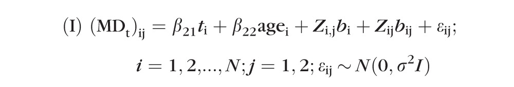where i and j are indices representing the subject identification and the eye (nested within subject), respectively. The β₂₁, β₂₂ are the slope and age effect, respectively; b_i and b_ij are first-level (subject) and second-level (eye within subject) random effects with corresponding matrices Z_i,j and Z_ij, respectively; and ε_ij values are within-group errors. The first level of random effect accounts for consistent differences in the MD between subjects. The second level of random effect accounts for consistent differences between the two eyes of a subject. The random effect is effectively an adjustment for the fact that some subjects will consistently have higher MD values than others, and it takes the form of a random variable, where there is one value for each subject.

The difference between model I and model II above is that here errors from model II are assumed to be temporally correlated according to a continuous autoregressive (CAR1) model with covariance matrix Σ₁, wherein the correlation between two residuals derived from the same eye decreases with the length of time between them. By contrast, errors are assumed to be uncorrelated within the same eye in model I.

Similarly, the following two-level (subject and eye within subject) exponential models were fitted to model nonlinearity in the MD data:

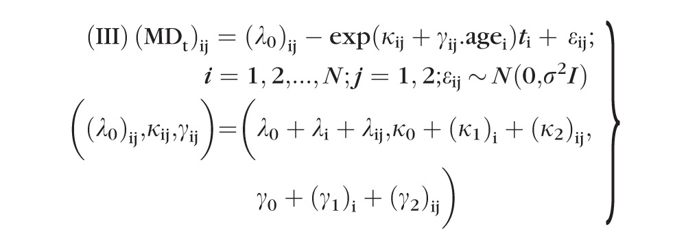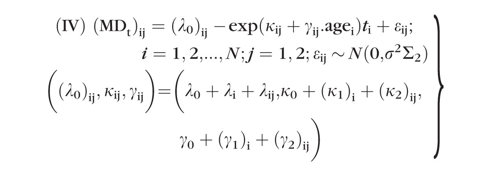For both model III and model IV, (λ₀, κ₀, γ₀,) are fixed-effects population parameters; b_i = (λ_i, (κ₁)_i, (γ₁)_i) and b_ij = (λ_ij, (κ₂)_ij, (γ₂)_ij) are level-one and level-two random effects, respectively; and ε_ij values are within-group errors. Similar to LME model II, the errors of model IV are assumed to be temporally correlated according to a continuous autoregressive (CAR1) model with covariance matrix Σ₂ (i.e., the correlation decreases exponentially with the length of time between the measurements), whereas errors are assumed to be uncorrelated for model III. All random effects (b_i, b_ij, ε_ij) were assumed to be independent. In addition, b_i values were assumed to be independent for different subjects, and b_ij and ε_ij were assumed to be independent for different subjects and/or different eyes.

References

- 1. Weinreb RN, Khaw PT. Primary and open-angle glaucoma. Lancet. 2004; 363: 1711–1720 [DOI] [PubMed] [Google Scholar]
- 2. Quigley HA, Broman AT. The number of people with glaucoma worldwide in 2010 and 2020. Br J Ophthalmol. 2006; 90: 262–267 [DOI] [PMC free article] [PubMed] [Google Scholar]
- 3. Strouthidis NG, Scott A, Peter NM, Garway-Heath DF. Optic disc and visual field progression in ocular hypertensive subjects: detection rates, specificity and agreement. Invest Ophthalmol Vis Sci. 2006; 47: 2904–2910 [DOI] [PubMed] [Google Scholar]
- 4. Kass MA, Gordon MO, Gao F, et al. Delaying treatment of ocular hypertension. Arch Ophthalmol. 2010; 128: 276–287 [DOI] [PMC free article] [PubMed] [Google Scholar]
- 5. Gardiner SK, John CA, Demirel S. Factors predicting the rate of functional progression in early and suspected glaucoma. Invest Ophthalmol Vis Sci. 2012; 53: 3598–3604 [DOI] [PMC free article] [PubMed] [Google Scholar]
- 6. Kulkarni KM, Mayer JR, Lorenzana LL, Myers JS, Spaeth GL. Visual field staging system in glaucoma and the activities of daily living. Am J Ophthalmol. 2012; 154: 445–451 [DOI] [PubMed] [Google Scholar]
- 7. De Moraes CG, Ghobraiel SR, Ritch R, Liebmann JM. Comparison of PROGRESSOR and Glaucoma Progression Analysis 2 to detect visual field progression in treated glaucoma patients. Asia Pacific J Ophthalmol. 2012; 1: 135–139 [DOI] [PubMed] [Google Scholar]
- 8. Smith SD, Katz J, Quigley HA. Analysis of progressive change in automated visual field in glaucoma. Invest Ophthalmol Vis Sci. 1996; 37: 1419–1428 [PubMed] [Google Scholar]
- 9. Gardiner SK, Crabb DP. Examination of different pointwise linear regression methods for determining visual field progression. Invest Ophthalmol Vis Sci. 2002; 43: 1400–1407 [PubMed] [Google Scholar]
- 10. De Moraes CG, Demirel S, Gardiner SK, et al. Ocular Hypertension Treatment Study Group. Rate of visual field progression in eyes with optic disc hemorrhages in the Ocular Hypertension Treatment Study. Arch Ophthalmol. 2012; 130: 1541–1546 [DOI] [PubMed] [Google Scholar]
- 11. De Moraes CG, Demirel S, Gardiner SK, et al. Ocular Hypertension Treatment Study Group. Effect of treatment on the rate of visual field change in the ocular hypertension treatment study observation group. Invest Ophthalmol Vis Sci. 2012; 53: 1704–1709 [DOI] [PMC free article] [PubMed] [Google Scholar]
- 12. Heijl A, Bengtsson B, Hyman L, Leske MC; Early Manifest Glaucoma Trial Group. Natural history of open-angle glaucoma. Ophthalmol. 2009; 116: 2271–2276 [DOI] [PubMed] [Google Scholar]
- 13. Russell RA, Crabb DP, Malik R, Garway-Heath DF. The relationship between variability and sensitivity in large-scale longitudinal visual field data. Invest Ophthalmol Vis Sci. 2012; 53: 5985–5990 [DOI] [PubMed] [Google Scholar]
- 14. Artes PH, Iwase A, Ohno Y, Kitazawa Y, Chauhan BC. Properties of perimetric threshold estimates from Full Threshold, SITA Standard, and SITA Fast strategies. Invest Ophthalmol Vis Sci. 2002; 43: 2654–2659 [PubMed] [Google Scholar]
- 15. Henson DB, Chaudry S, Artes PH, Faragher EB, Ansons A. Response variability in the visual field: comparison with optic neuritis, glaucoma, ocular hypertension and normal eyes. Invest Ophthalmol Vis Sci. 2000; 41: 417–421 [PubMed] [Google Scholar]
- 16. Leary N, Chauhan BC, Artes PH. Visual field progression in glaucoma: estimating the overall significance of deterioration with permutation analyses of pointwise linear regression. Invest Ophthalmol Vis Sci. 2012; 53: 6776–6784 [DOI] [PubMed] [Google Scholar]
- 17. Garway-Heath DF, Caprioli J, Fitzke FW, Hitchings RA. Scaling the hill of vision: the physiological relationship between light sensitivity and ganglion cell numbers. Invest Ophthalmol Vis Sci. 2000; 41: 1774–1782 [PubMed] [Google Scholar]
- 18. Hood DC, Kardon RH. A framework for comparing structural and functional measures of glaucomatous damage. Prog Retin Eye Res. 2007; 26: 688–710 [DOI] [PMC free article] [PubMed] [Google Scholar]
- 19. Harwerth RS, Wheat JL, Fredette MJ, Anderson DR. Linking structure and function in glaucoma. Prog Retin Eye Res. 2010; 29: 249–271 [DOI] [PMC free article] [PubMed] [Google Scholar]
- 20. Gordon MO, Beiser JA, Brandt JD, et al. The Ocular Hypertension Treatment Study: baseline factors that predict the onset of primary open-angle glaucoma. Arch Ophthalmol. 2000; 120: 714–720, 829–830 [DOI] [PubMed] [Google Scholar]
- 21. Bonomi L, Marchini G, Marraffa M, Bernardi P, Morbio R, Varotto A. Vascular risk factors for primary open angle glaucoma: the Egna-Neumarkt Study. Ophthalmology. 2000; 107: 1287–1293 [DOI] [PubMed] [Google Scholar]
- 22. Broadway DC, Drance SM. Glaucoma and vasospasm. Br J Ophthalmol. 1998; 82: 862–870 [DOI] [PMC free article] [PubMed] [Google Scholar]
- 23. Drance S, Anderson DR, Schulzer M. Risk factors for progression of visual field abnormalities in normal-tension glaucoma. Am J Ophthalmol. 2001; 131: 699–708 [DOI] [PubMed] [Google Scholar]
- 24. Leske MC, Connell AM, Wu SY, Hyman LG, Schachat AP. Risk factors for open-angle glaucoma: the Barbados Eye Study. Arch Ophthalmol. 1995; 113: 918–924 [DOI] [PubMed] [Google Scholar]
- 25. Gardiner SK, Johnson CA, Cioffi GA. Evaluation of the structure-function relationship in glaucoma. Invest Ophthalmol Vis Sci. 2005; 46: 3712–3717 [DOI] [PubMed] [Google Scholar]
- 26. Spry P, Johnson C, Mansberger S, Cioffi G. Psychophysical investigation of ganglion cell loss in early glaucoma. J Glaucoma. 2005; 14: 11–18 [DOI] [PubMed] [Google Scholar]
- 27. Chopra V, Varma R, Francis BA, Wu J, Torres M, Azen SP. Type 2 diabetes mellitus and the risk of open-angle glaucoma: the Los Angeles Latino Eye Study. Ophthalmology. 2008; 115: 227–232 [DOI] [PMC free article] [PubMed] [Google Scholar]
- 28. Anderson D, Patella V. Automated Static Perimetry. 2nd ed. St. Louis: Mosby; 1999. [Google Scholar]
- 29. Bengtsson B, Olsson J, Heijl A, Rootzén H. A new generation of algorithms for computerized threshold perimetry, SITA. Acta Ophthalmol Scand. 1997; 75: 368–375 [DOI] [PubMed] [Google Scholar]
- 30. Medeiros FA, Weinreb RN, Moore G, Liebmann JM, Girkin CA, Zangwill LM. Integrating event- and trend-based analyses to improve detection of glaucomatous visual field progression. Ophthalmol. 2012; 119: 458–467 [DOI] [PMC free article] [PubMed] [Google Scholar]
- 31. Demirel S, De Moraes CG, Gardiner SK, et al. Ocular Hypertension Treatment Study Group. The rate of visual field change in the Ocular Hypertension Treatment Study. Invest Ophthalmol Vis Sci. 2012; 53: 224–227 [DOI] [PMC free article] [PubMed] [Google Scholar]
- 32. R Core Team R: A Language and Environment for Statistical Computing. Vienna: R Foundation for Statistical Computing; 2013. Available at: http://www.R-project.org/. Accessed July 2, 2013 [Google Scholar]
- 33. Pinheiro JC, Bates DM. Mixed-Effects Models in S and S-plus. New York: Springer-Verlag; 2000. [Google Scholar]
- 34. Piltz JR, Starita RJ. Test-retest variability in glaucomatous visual fields. Am J Ophthalmol. 1990; 109: 109–111 [PubMed] [Google Scholar]
- 35. Shafi A, Swanson WH, Dul MW. Structure and function in patients with glaucomatous defects near fixation. Optom Vis Sci. 2011; 88: 130–139 [DOI] [PMC free article] [PubMed] [Google Scholar]
- 36. Caprioli J, Mock D, Bitrian E, et al. Author response: on alternative methods for measuring visual field decay: Tobit linear regression. Invest Ophthalmol Vis Sci. 2012; 53: 9211–9240 [DOI] [PubMed] [Google Scholar]
- 37. Russell RA, Crabb DP. A method of measuring and predicting rates of regional visual field decay in glaucoma. Invest Ophthalmol Vis Sci. 2011; 52: 9539–9540 [DOI] [PubMed] [Google Scholar]
- 38. Caprioli J, Mock D, Bitrian E, et al. A method to measure and predict rates of regional visual field decay in glaucoma. Invest Ophthalmol Vis Sci. 2011; 52: 4765–4773 [DOI] [PubMed] [Google Scholar]
- 39. Gardiner SK, Demirel S, Johnson CA. Is there evidence for continued learning over multiple years in perimetry? Optom Vis Sci. 2008; 85: 143–148 [DOI] [PMC free article] [PubMed] [Google Scholar]