Structure, Stiffness and Substates of the Dickerson-Drew Dodecamer

Abstract

The Dickerson–Drew dodecamer (DD) d-[CGCGAATTCGCG]₂ is a prototypic B-DNA molecule whose sequence-specific structure and dynamics have been investigated by many experimental and computational studies. Here, we present an analysis of DD properties based on extensive atomistic molecular dynamics (MD) simulations using different ionic conditions and water models. The 0.6–2.4-µs-long MD trajectories are compared to modern crystallographic and NMR data. In the simulations, the duplex ends can adopt an alternative base-pairing, which influences the oligomer structure. A clear relationship between the BI/BII backbone substates and the basepair step conformation has been identified, extending previous findings and exposing an interesting structural polymorphism in the helix. For a given end pairing, distributions of the basepair step coordinates can be decomposed into Gaussian-like components associated with the BI/BII backbone states. The nonlocal stiffness matrices for a rigid-base mechanical model of DD are reported for the first time, suggesting salient stiffness features of the central A-tract. The Riemann distance and Kullback–Leibler divergence are used for stiffness matrix comparison. The basic structural parameters converge very well within 300 ns, convergence of the BI/BII populations and stiffness matrices is less sharp. Our work presents new findings about the DD structural dynamics, mechanical properties, and the coupling between basepair and backbone configurations, including their statistical reliability. The results may also be useful for optimizing future force fields for DNA.

INTRODUCTION

The knowledge of DNA structure and physicochemical properties is indispensable for understanding its functional role in living organisms. Besides experimental techniques such as X-ray crystallography and NMR spectroscopy, molecular dynamics (MD) simulations provide valuable information. Modern atomic-resolution MD simulations with explicit representation of water and ions offer a detailed picture of atomic motions, which is very hard to obtain experimentally. The basic limitations of the MD technique are the approximate nature of the modeled interatomic potentials (force fields) and the limited time scale of the simulations.^1–3

In recent years, several large-scale MD studies of DNA have been performed. In particular, the ABC consortium^4–6 and the Sarai group^7,8 have simulated and analyzed B-DNA oligomers containing all of the 136 tetrameric base sequences. Orozco and co-workers reported the first microsecond MD simulation of a DNA oligomer.⁹ These and many other MD studies of DNA demonstrate the basic reliability of the technique and its applicability to a wide range of problems.

Nevertheless, a careful comparison of MD data with experimental results remains a topic of primary importance. It identifies the MD capabilities, delineates the limits of its use, and helps to design improved force fields and simulation protocols. One way this assessment can be done is to compare statistical properties of a set of simulated sequences to a set of crystal structures.^8,10 In this work, we pursue a different approach—we focus on one particular B-DNA oligomer and compare the simulated data with experimental information for the same molecule. The benchmark molecule we have chosen is the so-called Dickerson–Drew dodecamer.

There is hardly any other DNA oligomer which has been investigated to such an extent as the Dickerson–Drew dodecamer (DD), a prototypic B-DNA molecule of the sequence d[CGCGAATTCGCG]₂. It was the first DNA oligomer whose single crystal structure was determined,^11,12 revealing major sequence-dependent features that could not be observed in fiber diffraction studies of sequence-averaged B-DNA.¹² Since then, the molecule has been extensively studied by X-ray crystallography,^13–21 NMR spectroscopy,^22–24 and other biophysical techniques.^24–26 Recently, an NMR study of DD containing a single ribonucleotide was published.²⁷

A number of computational studies of DD have been performed. The pioneering molecular dynamics (MD) and continuum solvent simulations reported by Beveridge and co-workers²⁸ and Case and co-workers²⁹ accounted for experimentally observed conformational preferences and provided a physical explanation of the relative stabilities of A- and B-helices. The NOESY volumes and scalar coupling constants inferred from MD simulations of DD showed generally good agreement with the NMR data.³⁰ The first microsecond MD simulation of B-DNA by Perez et al.⁹ confirmed structure stability and revealed atomic-resolution dynamics of DD on an unprecedented time scale. The authors found agreement of many structural and dynamical features with experimental data.

Atomistic MD simulations are not just a source of detailed structural and dynamical information. They can also be used to parametrize DNA models on coarser scales. Structural analysis of the trajectory snapshots produces time series of generalized coordinates associated with the coarse-grained model, from which model parameters can be inferred. In particular, Lankas et al.³¹ proposed a nonlocal model of DNA shape and harmonic stiffness in which bases are represented as rigid bodies. This model extends earlier, local models of independent dinucleotide steps parametrized from an ensemble of crystal structures³² and from MD simulations,^7,8,33 as well as MD-parametrized local intra-base-pair stiffness models.^34,35 It builds on an earlier theoretical approach where DNA was treated as a chain of locally interacting rigid base pairs.³⁶

Here, we present an analysis of a new, 2.4 µs explicit-solvent MD trajectory of DD immersed in a water solution with a physiological KCl concentration. We also analyze another new, 0.6 µs MD trajectory of DD using different force field parameters for KCl, and the original 1.2 µs trajectory of Perez et al.⁹ which employs Na⁺ counterions and a different water model. In this way, a range of simulation conditions has been covered. We provide extensive comparison with modern X-ray and NMR structural data in terms of intra-base-pair, base-pair step, and backbone conformational parameters. We focus on the BI/BII backbone substates and their influence on the oligomer structure. Apart from structure and dynamics, we infer, for the first time, mechanical properties of DD using a nonlocal harmonic model of rigid bases closely analogous to that of Lankas et al.³¹ We report in detail various features of the nonlocal stiffness matrices. To compare the stiffness matrices, we employ the Riemann distance and Kullback–Leibler divergence, earlier used in the theory of averaging of stiffness tensors.37–39 In all cases, we pay particular attention to the problem of convergence of the studied quantities.

METHODS

All the simulated data were obtained from atomic-resolution MD trajectories of DD with explicit representation of water and ions. The AMBER suite of programs together with the parmbsc0 force field for DNA⁴⁰ was used in all cases. The new 2.4 µs trajectory (KCl_Dg) was obtained using the SPC/E water model, K⁺ counterions to neutralize the DNA charge, and 150 mM added KCl. The ions were parametrized according to Dang.⁴¹ This setup exactly corresponds to the one used in the latest large-scale simulation study of the ABC consortium.⁶ Another, 0.6 µs trajectory (KCl_JC) was produced using the same setup but taking the K⁺ and Cl⁻ parameters of Joung and Cheatham.⁴² We also analyzed the 1.2 µs trajectory of Perez et al.,⁹ which was obtained using the TIP3P water model and the Na⁺ counterions only, with the default parm99 parameters for the ions. In the case of KCl_Dg and KCl_JC simulations, the protocol for building the system and performing the simulation was identical to that used in the latest ABC study,⁶ the Perez et al. protocol was similar.⁹ The simulations are summarized in Table 1. Besides that, we also performed an additional 1.7 µs control simulation of DD capped with G—C pairs at both ends, i.e., the 14-mer d[GCGCGAATTCGCGC]₂. The simulation conditions were exactly analogous to those of KCl_Dg.

Table 1.

Overview of the Simulations and Lifetimes of the WW and TT States

simulation code	simulation time (ns)	salt	ion parameters	water model	time in WW state (ns)	time in TT state (ns)	% in WW state	% in TT state
KCl_Dg	2400	150 mM KCl	Dang	SPC/E	265	381	11	16
KCl_JC	600	150 mM KCl	Joung and Cheatham	SPC/E	330	0	55	0
Na—Bsc	1200	Na+	parm99	TIP3P	225	643	19	54

Snapshots taken in 10 ps intervals were analyzed using the 3DNA program.⁴³ From 3DNA outputs, time series of conformational parameters were extracted. These included the intra-base-pair coordinates (buckle, propeller, opening, shear, stretch, and stagger), inter-base-pair or step coordinates (tilt, roll, twist, shift, slide, and rise) as well as groove widths (based on P—P distances), backbone torsions, and sugar puckers.

Stiffness Analysis

The mechanical properties of DD were described using a harmonic, nonlocal rigid base model as proposed by Lankas et al.³¹ In this model, the internal elastic energy (or deformation energy) U of the oligomer is of the general quadratic form

$$U(\mathbf{w})=\frac{1}{2}(\mathbf{w}-\widehat{\mathbf{w}})\cdot \mathbf{K}(\mathbf{w}-\widehat{\mathbf{w}})$$ (1)

where w is the vector of intra-base-pair and step coordinates of the oligomer, ŵ is a vector of coordinate values defining the energy minimum (shape parameters), and K is a symmetric, positive definite stiffness matrix. The model parameters ŵ and K are related to the statistical moments of the coordinates.³¹ These relations include a Jacobian factor due to the non-Cartesian nature of the rotational coordinates. If the fluctuations of these coordinates are small, the Jacobian can be assumed constant, and the relations take the form³¹

$$\widehat{\mathbf{w}}=\langle \mathbf{w}\rangle ,\mathbf{K}=k_{\mathrm{B}}T{\mathbf{C}}^{-1}$$ (2)

where 〈•〉 denotes the average over the canonical ensemble, C is the coordinate covariance matrix, k_B is the Boltzmann constant, and T is the thermodynamic temperature of the ensemble. Thus, the minimum energy shape parameters are just the means of the coordinates, and the stiffness matrix is proportional to the inverse of the covariance matrix. In our analysis, we replace the ensemble averages in eq 2 by the averages over the simulated trajectory. Contrary to the original work of Lankas et al.,³¹ the intra-base-pair and step coordinates used here are those defined by 3DNA.⁴³

Since the translational coordinates are measured in Ångstroms and the rotational ones in degrees, the entries of the stiffness matrix each have one of three different dimensions. To be able to analyze the stiffness matrix as a whole (e.g., in terms of eigenvalues and eigenvectors), we nondimensionalize and scale (or reduce) the matrix entries using the length scale of 1 Å and the angle scale of 10.6°. These values are inspired by the canonical B-DNA structure where the neighboring base pairs are 3.4 Å apart and twisted by 36°. Interestingly, a very similar scaling can be deduced if we consider the dimensions of a single base pair: the length (C6–C8 distance) of a canonical Watson-Crick pair is 10 Å;⁴⁴ thus turning it by 10.6° about an axis passing through the midpoint and perpendicular to C6–C8 displaces these atoms by 0.93 Å.

In order to easily compare two stiffness matrices, it is preferable to define a distance between them. Lankas et al.³¹ used the Euclidean (or Frobenius) norm, defined for any matrix. However, it might be more appropriate to use a distance which is natural to symmetric positive definite matrices. The question of the appropriate metric was studied by Moakher^37,38 and Moakher and Batchelor³⁹ in connection with the problem of averaging of symmetric positive definite tensors. The authors notice that the set of symmetric positive definite matrices of dimension n by n, denoted P(n), is a differentiable manifold immersed in the space of all nonsingular matrices of the same dimension. The geodesic (or Riemannian) distance between matrices K₁ and K₂ in P(n) is given by

$$d_{\mathrm{R}}({\mathbf{K}}_1,{\mathbf{K}}_2)={[\sum _{i=1}^n{(\text{ln}{\lambda }_i)}^2]}^{1/2}$$ (3)

where λ_i are the (positive) eigenvalues of K₁⁻¹K₂.³⁷⁻³⁹

Another suitable measure of a deviation between symmetric positive definite matrices can be defined using the Kullback–Leibler divergence, employed in information theory to measure the difference between two probability distributions.^38,39Consider two zero-mean Gaussian distributions with inverse covariance matrices K₁ and K₂. The symmetrized Kullback–Leibler divergence between the two distributions has the form

$${\text{KL}}_{\mathrm{s}}({\mathbf{K}}_1,{\mathbf{K}}_2)=\frac{1}{2}\sum _{i=1}^n{(\sqrt{{\lambda }_i}-\frac{1}{\sqrt{{\lambda }_i}})}^2$$ (4)

where λ_i has the same meaning as in eq 3. This quantity behaves similarly to a square of a distance;³⁹ therefore we use the square root of it:

$$d_{\text{KL}}({\mathbf{K}}_1,{\mathbf{K}}_2)=\sqrt{{\text{KL}}_{\mathrm{s}}({\mathbf{K}}_1,{\mathbf{K}}_2)}$$ (5)

which we will call the KL divergence.

RESULTS

In this section, we present the major results concerning the DD structure, dynamics, conformational substates, mechanical properties, and convergence.

The End Bases Can Adopt a Non-WC Pairing in MD

The first feature to note is that the simulated DD, in all of the MD simulations studied here, exhibits two types of pairing of the end bases (Figure 1, Table 1, Figure S1). Besides the usual Watson–Crick (WC) pairing or unpaired bases, the end cytosine can also turn around the glycosidic bond from the anti to syn conformation to form a non-WC pair, which resembles a trans Watson–Crick/sugar edge (tWS) C–G pair well-known from RNA structures.⁴⁵ This noncanonical pair is further stabilized by the O5′···O2 intranucleotide hydrogen bond within the cytidine. In this way, the total number of hydrogen bonds stays the same as in the original WC C–G pair. The phenomenon is illustrated in Figure 1 for the KCl_Dg simulation. One of the ends switches from the WC pairing to the tWS one at 265 ns and is thus in tWS for most of the simulation time, whereas the other end switches at ca. 2000 ns and is therefore in WC for most of the time. This change is reflected in the conformational parameters. For instance, twist averaged over the whole trajectory shows values characteristic for the WC pairing at one end and those of the tWS pairing at the other end (Figure 1). The difference attains as much as 7° of twist for the inner CG steps.

Figure 1.

End pairing and its effect on the helical structure. The bases at the oligomer ends can either form a WC pair (top left) or a tWS pair, additionally stabilized by the intranucleotide O5′···O2 hydrogen bond (top right). In the course of the simulation, the WC end pairs (bottom left, green) are rather unstable (unpaired bases, dark red) and eventually flip to tWS pairs on both ends (yellow). The end pairing has a strong effect on the oligomer conformation up to the inner CG steps (third steps from the ends). For instance, twist (bottom right) in CG steps differs by 5–7° between the state where each end is either WC-paired or unpaired (WW state, green) and the one where both ends form tWS pairs (TT state, yellow). The mean over the whole trajectory (red) is asymmetric, reflecting a mixture of the end pairings. The outer CG steps are not shown in the twist plot. The data are for the KCl_Dg simulation. Plots analogous to the bottom left panel for the other simulations are in Figure S1.

Backward tWS to WC changes occur in the Na_Bsc simulation (Figure S1), but the very long lifetimes of the alternative pairing states compared to the simulation time prevent us from characterizing the statistics of the alternative pairing in any definitive way.

Given the long lifetimes of the end pairing states and their effect on conformation, we decided to analyze them separately. We distinguish two cases: in the first state (WW in Figure 1), each end is either WC paired or unpaired; in the second state (TT in Figure 1), both ends are tWS paired. The total simulation times spent in the WW and TT states are in Table 1. There is no TT state in the KCl_JC simulation. The conformations where each end is in a different state would probably be a mixture of the WW and TT states, as suggested by the twist profile in Figure 1. However, it is not a priori clear how deeply the end state effects propagate into the oligomer. Thus, we adopted a conservative approach and only analyzed conformations where both ends are in the same state; i.e., we consider either WW or TT states.

From now on, unless otherwise stated, all the results we present in the main text have been obtained for the WW state. Data for the TT state are presented in the Supporting Information.

To investigate the end effects further, we performed an additional microsecond-long simulation of DD capped by G–C pairs at each end, resulting in the d[GCGCGAATTCGCGC]₂ 14-mer (see Methods). In this case, the ends showed entirely different behavior. The WC pairing at one end just occasionally broke and reformed, leaving the neighboring pair intact. Substantial fraying, however, was seen at the other end: 1–2 pairs were broken and the terminal 3′-C transiently folded back onto the oligomer, interacting with third–fourth pair in the minor groove. The 5′-terminal G does not form any stable intramolecular H-bond. Notice that 5′-terminal deoxyribogua-nosine can flip to syn and form an efficient 5′OH···N3 intramolecular H-bond, as evidenced by simulations of quadruplex DNA (G-DNA) stems.⁴⁶ Such H-bonds also form in experimental G-DNA structures if there is no loop or flanking nucleotide upstream of the G-tract and substantially affect the topology of the G-DNA stems by reversing the stability order of anti and syn guanine arrangements.² However, in our simulations we have seen only occasional flips of the 5′-terminal G to syn and only transient formation of the 5′OH···N3 H-bond. The most likely reason why the C–G to G–C reversal of the terminal base pair affects the behavior of the duplex end is not the inability of the G nucleoside to form a stable intramolecular H-bond in the syn conformation but the low stability of the potential tWS G–C base pair, which would have only one H-bond in DNA.⁴⁵ A better pairing could be achieved via the trans Watson–Crick/Watson–-Watson–Crick donor–acceptor pattern, but that would require a substantial repositioning of the two terminal nucleosides. Alternatively, the Hoogsteen edge of guanine could pair with cytosine, but this would require N3 protonation of the cytosine, as known from triplexes.

Structural Parameters Compared to Experimental Results

We compare the structural parameters from the three simulations to experimental data. We have chosen four high-resolution crystal structures and one high-quality NMR structure for the comparison. All of these experimental structures have either WC pairs or unpaired bases at the ends.

A number of X-ray structures of DD have been published. We focus on more recent studies, since their accuracy and precision are better compared to older ones due to high-quality diffraction, high-precision nucleotide geometry, and sophisticated refinement methods.¹² The oligomers in the crystals are subjected to lattice interactions (packing forces) whose effect on the DD conformation has been extensively discussed.^12,47 In particular, the conformations are influenced by the space group in which the oligomer crystallizes.^12,47 We have chosen the very high-resolution structure of Tereshko et al.¹⁵ (1.1 Å, NDB code BD0007) and the K⁺ form of DD by Sines et al. (1.2 Å, BD0041) as representatives of the most common P2₁2₁2₁ group. Besides that, we consider the Johansson et al.²⁰ structure crystallized in the 2-fold symmetric P3₂12 group (1.8 Å, BD0032) and the Liu and Subirana¹⁶ structure which, in the presence of Ca²⁺ ions, crystallized in the H3 group (1.45 Å, BD0014).

NMR experiments are done in solution, thus the oligomer is not affected by the packing forces. However, the resulting structure may be influenced by the refinement procedure. Wu et al.²³ reported a solution structure of DD determined on the basis of an exceptionally large set of constraints. In particular, the large number of homo- and heteronuclear dipolar couplings strongly reduces the dependence of the solved structure on technical details of the refinement. This is corroborated by the fact that turning off the electrostatic term has a minimal effect on the refined structure.²³ We consider this DD structure (pdb code 1NAJ, 5 models) as a reference for the DD structure in solution.

The average intra-base-pair and step coordinates are shown in Figures 2 and 3 and listed in Tables S1 and S2. Values for the inner octamer only are shown. We see that some important features are qualitatively similar among all the structures, both MD and experimental. In particular, the high positive roll, small slide, and small propeller in the C/G regions are contrasted with the zero or negative roll, high negative slide, and high negative propeller in the central A/T part. However, significant differences between different structures are also apparent. Individual crystal structures show a wide variety of values, most likely reflecting the effect of packing forces as well as divalent ions found at various locations in most of the structures.

Figure 2.

Inter-base-pair (or step) coordinates. Four X-ray structures crystallized in three different space groups and one high-quality NMR structure (mean parameters over the NMR models) are compared to averages from three MD trajectories obtained using different simulation conditions (Table 1). Overall qualitative similarities as well as important differences are seen, for instance in the CG steps. Notice the variability among the crystal structures even in the central part of the oligomer. Only the central octamer is shown. The nomenclature is described in the text. The error estimates for the MD data are omitted for clarity, but the convergence is excellent—see Figure 9 and Table S1. Only the trajectory portions in the WW end state (Figure 1) are considered. Comparison to MD values for the TT state is in Figure S2.

Figure 3.

Intra-base-pair coordinates. Values were obtained as in Figure 2. The high negative propeller in the NMR solution structure is not attained by any of the MD simulations. MD data are for the WW state; comparison to the TT state data is in Figure S3.

For a relaxed palindromic sequence, the coordinate values must be symmetric with respect to the oligomer center, with the exception of tilt, shift, buckle, and shear, which must be antisymmetric.³¹ None of the X-ray structures shows these symmetries except for the one crystallized in the P3₂12 group²⁰ where the exact symmetry is dictated by the space group itself. The NMR structure shows an almost perfect symmetry, together with lower variation of the parameters, as expected for a relaxed structure. The MD data fulfill the symmetry requirements very well. Furthermore, values for different MD simulations are quite close to each other, despite the differences in simulation conditions (different solvent composition, concentration and parametrization of ions, and different water models), supporting the robustness of the technique.

Interesting features are related to twist, a parameter long suspected to be underestimated by MD simulations. Fujii et al.⁸ compared a set of simulated oligomers covering all the tetrameric sequences to an X-ray structural database⁴⁸ and found an underestimation of twist in pyrimidine–purine (YR) steps. These results were based on rather short MD trajectories obtained using the older parm99 force field. However, Perez et al.⁴⁹ performed much longer simulations with the current parmbsc0 force field and also found twist underestimation for several dinucleotide steps including the YR ones. Our data indicate that the simulated twist in DD is indeed underestimated in all the steps except GA. The most striking behavior is observed for the CG steps, where the MD twist is around 25°, whereas the twist of the relaxed NMR structure is 34°; interestingly, all the X-ray structures show values around 25°, close to the MD ones but at variance with NMR.

Fujii et al.⁸ also found that the (signed) values of slide based on MD are lower than the X-ray ones for all the dinucleotide steps, an effect confirmed by the Perez et al.⁴⁹ parmbsc0 data. Our simulated slide in DD is mostly lower than the X-ray values, but the discrepancy is limited to the A/T region if compared to NMR data. Contrary to twist, MD slide values in the CG steps agree with NMR but disagree with the X-ray data.

An important conformational parameter is propeller. Its high negative values are characteristic for DNA A-tracts, sequences of at least four A–T pairs without a TA step (see, e.g., a recent study⁵⁰ and references therein). The ability of a force field to reproduce high negative propeller in A-tracts is a critical test of the force field quality.⁵¹ Propeller in the central A-tract of DD is −20° or less negative for both X-ray and MD data, whereas NMR values attain −23°. Thus, MD slightly underestimates (by 3°) the A-tract propeller in DD with respect to the reference NMR structure. Significant differences are also observed for rise, stretch, and other parameters (Figures 2 and 3).

The major and minor groove width profiles are shown in Figure 4. Both experimental and MD data indicate minor groove narrowing in the central A-tract, a feature typical for A-tracts and seen already in the first crystal structure of DD.¹² The major groove profiles are more variable, but all show narrowing around the central AT step. The MD minor and major grooves are generally wider compared to the experimental data, a fact already found by Perez et al. (see Figure 3 in ref 49) and recently observed also for RNA⁵²

Figure 4.

Minor and major groove widths. Values were obtained as in Figure 2. The MD simulations mostly yield wider minor and major grooves than the experimental structures. MD data are for the WW state; values for the TT state are very similar.

Figure 5 shows profiles of the glycosidic χ angles and sugar puckers in the central octamer. The χ angles are all in the anti conformation, with mostly lower values in the A/T part than in the G/C parts. The puckers are mostly in the south to southeast region, with generally lower values for pyrimidines than for purines, as previously observed.²³ Due to the palindromic sequence, the profiles of χ and pucker for the two strands, both taken in the 5′ to 3′ direction, should be identical. The profiles indeed differ only slightly (or are identical by definition as in P3₂12 and NMR); therefore we plot just the average values of the two strands.

Figure 5.

Glycosidic angles and sugar puckers. Nomenclature is as in Figure 2. Averages of the values in the two strands are plotted. Only the WW state MD data are shown; the TT values differ by no more than 10°.

The authors of the NMR study²³ interpret their structural data in terms of a two-state model capturing the north–south (N–S) exchange of the puckers. A similar approach was used earlier.⁵³ We tried to identify the N and S substates by plotting the pucker histograms for all the sugars individually. However, in no single case did we see separate peaks in the N and S regions. Rather, there was always only one peak (or two closely located peaks) in the south to southeast region, with a long tail extending to the N region. It is not clear if the discrepancy between MD and NMR data found here is due to a shortcoming of the force field or to the assumption of two states in the interpretation of the NMR data (east sugar conformers are not rare in B-DNA crystal structures).

BI/BII Populations Show Strong Sequence Dependence

We observe interconversions between the backbone substate BI (the ε/ζ backbone torsions in the t/g+ state) and BII (ε/ζ torsions in g+/t). The BII populations are shown in Figure 6. Since the sequence is palindromic, the profiles for the two strands should be identical. The MD data for the two strands are indeed quite close; thus we plot only the average values of the two strands. There is only one backbone fragment (single-strand step) with high BII content observed in MD, namely the G4–A5 (or equivalently G16–A17) step.

Figure 6.

Populations of the BII substate. Experiment-based values from three studies (see text) are compared to MD data. Mean values for the two strands are shown. The crosses indicate maximum and minimum values for the two halves of each trajectory and each strand (MD data) or published error estimates (experiment-based data). Heddi et al. report the error in their data to be 8% BII on average. Although all the data indicate lower BII content in the central A/T region than in the flanking C/G parts, the variability between the experiment-based data and the difference between experimental data and MD are substantial. MD data are for the WW state. The TT values are very similar, except that the TT Na_Bsc simulation has 25% BII in the C9-G10 step (on the right in the Figure).

Schwieters and Clore²⁴ performed an NMR experiment on DD together with large-angle solution X-ray scattering measurements and estimated the BII populations. Tian et al.⁵⁴ inferred the populations from NMR measurements of DD using a two-state model. Heddi et al.⁵⁵ observed correlations between three interproton distances, phosphorus chemical shifts (δP), and BI/BII populations in X-ray structures and NMR, which enabled them to propose a linear relationship between δP and the BII percentage and to estimate the BII populations for the 16 single-strand dinucleotide steps.

The MD and the experiment-based data in Figure 6 both indicate that there is less BII in the central A/T part than in the flanking G/C parts. The estimated BII populations of Schwieters and Clore and our MD data are at least qualitatively comparable, both showing a peak in the G4–A5 step. This is not the case for the DD data of Tian et al., nor for the context-independent dinucleotide values of Heddi et al. (we show their newer, slightly modified values⁵⁶) which predict the CG steps to have the highest BII percentage. Heddi et al.⁵⁶ also consider context dependence in terms of purine (R) vs pyrimidine (Y) nucleotides flanking the step, but taking this into account would change the values only slightly (see Figure 3 in their study⁵⁶). In sum, uncertainties still exist about the BI/BII populations in DD. Nevertheless, it seems that MD with parmbsc0 might underestimate the BII percentage in some steps of DD, especially in CG steps. It is worth noting that BII states are rather short-lived in our MD, in agreement with previous findings.⁹ The average lifetime of the BII state within the inner octamer is tens to hundreds of picoseconds depending on the site, and the maximum lifetime does not exceed 9 ns.

Effect of BI/BII Substates on the Helical Structure

The two backbone fragments connecting the base pairs in a dinucleotide step can each be either in the BI or in the BII state. Thus, one can distinguish the step substates of BI/BI, BII/BII, and BI/BII or mixed. It has long been known that the inter-base-pair coordinates of the step change with these backbone substates. On the basis of a statistical analysis of X-ray data, Djuranovic and Hartmann discovered that passing from BI/BI to mixed to BII/BII substates implies a decrease in roll and increase in twist.⁵⁷ The data reported by Heddi et al. (see Figure S2 in ref 56) indicate that slide increases, too.

The corresponding data based on our MD simulations (Figure 7) fully confirm these trends. The decrease in roll and increase in twist and slide are observed for all the steps, although the magnitude of the change is somewhat sequence dependent. Besides that, we also observe an increase in rise for the CG steps and increase in the absolute values of tilt and shift (except steps where they are zero as a consequence of their antisymmetry—see above³¹). These phenomena, to our knowledge, have not been reported before. The BII/BII states are rare and are not shown in the figure, but in steps where they occur, they follow the same trends (i.e., an even larger change in the same direction as for BI/BII).

Figure 7.

Dependence of the average step coordinates on the backbone substates of the same step. The two backbone fragments of the step can be both in BI (BI/BI, continuous lines) or one of them in BI and the other in BII (mixed, BI/BII, broken line) or both in BII (BII/BII). The BI/BII state implies higher twist and slide and lower roll compared to BI/BI. It also increases rise (particularly in CG steps) and the absolute value of tilt and shift. The BII/BII states are rare, but in steps where there are enough of them, they imply even larger changes following the same trends (not shown). Only the values for the WW end states are plotted; the TT values show the same trends.

Parameter Distributions Are Sums of Gaussians Corresponding to BI/BII Substates

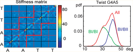
Several recent MD studies of B-DNA reported anharmonic (non-Gaussian) distributions of conformational parameters, notably twist.^6,9 Our MD data of DD exhibit Gaussian-like distributions for most of the parameters. Slide and especially twist do show anharmonicity (Figure 8). The anharmonic form of the G4A5 twist distribution (left panel) can be decomposed into Gaussian-like distributions corresponding to the BI/BI and BI/BII substates of that step. For twist in the C3G4 step (right panel), the distribution for the BI/BI substate is still rather anharmonic but can be further decomposed into two Gaussians corresponding to the BI and BII states of the neighboring G4–A5 backbone fragment. The BII/BII substate is very rare and does not play any significant role in the decompositions shown in the figure.

Figure 8.

Probability density functions of twist in the G4A5 and C3G4 steps from the KCl_Dg simulation. Twist of G4A5 (left, red line) is moderately anharmonic but can be decomposed into harmonic (Gaussian) contributions corresponding to the BI/BI and BI/BII states of the step. Twist of C3G4 in the BI/BI state (right, green line) is still anharmonic but can be further decomposed into harmonic contributions depending on the BI or BII state of the G4–A5 backbone fragment in the 3′ neighboring step. The BII/BII states are rare in all cases and contribute negligibly to the decomposition. Other coordinates in this and the other simulations either show analogous decomposable anharmonic behavior or are harmonic. Only the WW end states are considered; the TT state distributions are very similar.

Structural Differences between MD Simulations Are Small but Statistically Significant

To assess convergence of our structural parameters, we computed them separately for the first and the second halves of each MD trajectory (considering only WW end states as described above). As seen in Tables S1 and S2, the intra-base-pair and step parameters converge very well. Indeed, the error estimates are typically a fraction of a degree for rotational parameters and well below 0.1 Å for translational ones. This enables us to quantitatively compare the MD simulations which differ from each other in the type and parametrization of the ions and in the water model. The profiles of selected parameters are shown in Figure 9. Crosses indicate values for the two halves of each trajectory. Despite the overall similarity, the KCl_JC simulation (ions according to Joung and Cheatham, Table 1) clearly differs from the others: it exhibits, e.g., a more negative propeller in the A/T part and higher twist in GA steps.

Figure 9.

Convergence of selected coordinate averages. Crosses indicate values for the first and the second half of each trajectory (WW state only). Each of the MD trajectories was performed using different simulation conditions (Table 1). The excellent convergence enables one to identify small but statistically significant differences between individual simulations. The full list of average coordinates with error estimates is in Tables S1 and S2. The TT state values converge equally well.

The convergence of the BII populations (Figure 6) is not quite as sharp, especially in the highly populated G4–A5 fragment. Nevertheless, the KCl_JC simulation again stands out in predicting an even higher BII percentage in G4–A5 than the other simulations.

Stiffness

The nonlocal, rigid base harmonic stiffness model proposed by Lankas et al.³¹ assumes the elastic energy to be a general quadratic function of all the intra-base-pair and step coordinates. Thus, any base can in principle interact with any other base, and all the couplings between various coordinates, including those belonging to different base pairs and steps, are automatically taken into account. Here, we apply this model together with the 3DNA definitions of the intra-base-pair and step coordinates.⁴³ We only consider the coordinates within the inner octamer of the DD (90 coordinates in total). Since the fluctuations of the rotational coordinates within the octamer are small (standard deviations of several degrees), we neglect the effect of the Jacobian factor. The minimum energy coordinates (or shape parameters) are then just the coordinate means discussed above, and the stiffness matrix is proportional to the inverse of the covariance matrix (eq 2).

To compare the stiffness matrices from different MD simulations, we first look at their diagonal entries (Figures 10 and 11). The values are rather well converged, and we again observe small, statistically significant differences between the individual simulations. Symmetry with respect to the oligomer center³¹ is satisfied quite well. The diagonal entries have a straightforward physical meaning, following from eq 1: they are stiffness constants for deformations in which only the given coordinate changes, while all the other coordinates are kept at their equilibrium values. Figures 10 and 11 show that the central A-tract is in general stiffer than the flanking G/C parts with respect to these deformations. Notable exceptions are deformations in stretch and opening for which the A-tract is more flexible than the G/C parts. The reason might be that stretch and opening primarily change the geometry of the intra-base-pair hydrogen bonds, and smaller stiffness of the A/T pairs simply reflects the lower number of hydrogen bonds connecting the bases.

Figure 10.

Diagonal entries of the stiffness matrices corresponding to inter-base-pair (or step) coordinates. Only coordinates within the central octamer were used to compute the stiffness matrix. The diagonal entries are stiffness constants associated with a deformation in which only the given coordinate is changed while all the others are fixed in their equilibrium values. For these deformations, the central A-tract is stiffer than the flanking G/C parts for all the step coordinates. For a palindromic sequence, the values should be symmetric with respect to the oligomer center, which the data satisfy rather well. Crosses indicate values for the two halves of the trajectory. Although the convergence is not as clear-cut as for the coordinate averages (Figure 9), there are statistically significant differences between the simulations, with KCl_JC being the stiffest and Na_Bsc the most flexible. Only the WW end state is considered in each case. Comparison to the TT state data is in Figure S4.

Figure 11.

Diagonal entries of the stiffness matrices corresponding to intra-base-pair coordinates. See Figure 10 for details. The values are higher for the central A-tract than for the flanking G/C portions, with the exception of the stretch and opening stiffness. Just as for the step coordinates (Figure 10), the values converge rather well and expose differences between the simulations. Values for the palindromic sequence should be symmetric with respect to the oligomer center, which the data satisfy quite well. Only the WW end states are considered. Comparison to the TT state data is in Figure S5.

The stiffness matrix is fully characterized by its eigenvalues and eigenvectors. For their meaningful computation, the matrix must first be made dimensionally uniform, which we achieve by nondimensionalization and scaling (or reduction) as described in Methods. Numerically, the reduction means leaving the translational entries intact, multiplying the rotational ones by (36/3.4)² ≈ 100 and the mixed ones by 36/3.4 ≈ 10. Thus, the differences between the original translational and rotational entries (Figures 10 and 11) greatly diminish in the reduced matrix. The original matrix is already safely invertible. Indeed, its condition number is on the order of 10⁴ and further diminishes to 10² upon reduction.

The eigenvalues (Figure 12) again converge reasonably well and indicate differences between the simulations: the KCl_JC simulation predicts the stiffest oligomer (highest eigenvalues for all modes), followed by KCl_Dg, with Na_Bsc being the softest. Notice the dramatic change of the overall line slope around the 65th mode which can be interpreted as a separation between soft and hard modes.

Figure 12.

Eigenvalues of the stiffness matrices inferred from the simulations. The initial part of the graph is magnified in the inset. The broken lines indicate values for the two halves of each trajectory. The matrices have been nondimensionalized and scaled (or reduced) as described in the text. The data clearly identify small differences between the simulations: KCl_JC predicts the stiffest oligomer (highest eigenvalues for all modes), followed by KCl_Dg and Na_Bsc. For a given simulation, the stiffness ratio between the softest and the stiffest modes is roughly 1:250. The abrupt change in the slope around mode 65 may be interpreted as a boundary between soft and hard modes. Only the WW end states are considered. Comparison to the TT state data is in Figure S6.

Comparing the eigenvectors between the whole trajectory and its first half (Figure 13, left panel), we observe good convergence: the eigenvectors for the corresponding modes point mostly in very similar directions, with several swaps between neighboring modes. More differences are seen when comparing two different simulations (Figure 13, right panel).

Figure 13.

Scalar products between eigenvectors of the stiffness matrices. Absolute values of the scalar products are shown. On the left, the stiffness matrix eigenvectors for the KCl_Dg trajectory are compared to those for its first half. The vectors are shown in the order of increasing eigenvalues. If the two ensembles were identical, there would be just ones on the diagonal and zeros elsewhere. It is indeed almost the case, with the exception of several swapped modes having entries close to one next to the main diagonal and close to zero on the diagonal. The comparison of the KCl_Dg and Na_Bsc simulations (right) shows most nonzero entries within a narrow band around the diagonal, indicating that the modes are similar but not identical. Only the WW state is considered throughout; analogous data for the TT state are in Figure S7.

Table 2 shows the differences between the stiffness matrices expressed as Riemann distances and KL divergences, as described in the Methods. Again, the differences within one simulation (diagonal entries in the Table) are smaller than differences between simulations, but only by a factor of about two. Thus, the matrices can be considered converged, but the convergence is not absolutely clear-cut. Notice that the Riemann distance and KL divergence measure the difference between two stiffness matrices. They say nothing about which of the two is “stiffer”, or which entries contribute most to the difference.

Table 2.

Riemann Distances and KL Divergences between Stiffness Matrices Computed from the Whole MD Trajectories and from the Trajectory Halves (Diagonal Entries), and between Stiffness Matrices from Different Trajectories^a

	Riemann distance			KL divergence
	KCl_Dg	KCl_JC	Na_ Bsc	KCl_Dg	KCl_JC	Na_ Bsc
KCl_Dg	0.77, 0.78	2.15	2.18	0.55, 0.56	1.54	1.56
KCl_JC		0.96, 1.04	2.82		0.68, 0.74	2.03
Na Bsc			0.96, 1.23			0.68, 0.89

^aOnly the WW end state is considered. Analogous data for the TT state are in Table S3.

It is expected that base–base interactions diminish with the distance between the bases. The stiffness model used here includes all the base–base interactions; thus various simplified interaction patterns can be readily assessed. Lankas et al.³¹ proposed a nearest neighbor interaction model in which each base interacts only with its nearest neighboring bases within the same strand and in the opposite strand (thus, any nonterminal base has five interaction partners). This model implies a stiffness matrix which has nonzero entries only within a certain region around the main diagonal. The stiffness matrices from all the simulations appear to have most of the significantly nonzero entries within that region (Figure 14).

Figure 14.

A zoom-in of the central part of the stiffness matrix in its reduced form inferred from the KCl_Dg simulation (WW state only). The coordinates are ordered as follows: the six columns above the nucleotide symbol correspond to the intra-base-pair coordinates of that pair (buckle, propeller, opening, shear, stretch, and stagger); the six columns to the right correspond to the six coordinates of the 3′-adjacent base-pair step (tilt, roll, twist, shift, slide, and rise). By far the biggest entries (orange dots) are the diagonal stiffness constants for stretch and rise. The nearest-neighbor base–base interaction model predicts nonzero entries only within the region marked by the red lines. It is seen that most of the significantly nonzero entries are indeed found in this region.

Effect of Broken H-Bonds and Noncanonical α/γ Flips

The hydrogen bonds (H-bonds) keeping the WC pairs together occasionally break and reform. The transient H-bond breaks have already been observed in MD of B-DNA.^9,31 In line with the previous MD results, we found that the lifetimes of the broken H-bonds are typically 50 ps or smaller but can attain hundreds of picoseconds in isolated cases (max. 790 ps in our data). In general, H-bonds facing the major groove are more vulnerable to breaking. Notice that this phenomenon is different from the base-pair breathing measured in imino proton exchange experiments, where the base-pair lifetimes are roughly 100 ms and the open state lifetimes are on the order of 10 ns.⁵⁸

Another structural deviation common in simulations is the flip of the backbone torsion angles α/γ from the canonical g⁻/g+ state to the noncanonical g+/t (that is, both angles flip) or, very rarely, g⁻/t (only γ flips). While these alternative conformations are rather common in protein–DNA complexes,⁵⁹ they are only found in naked B-DNA crystal structures in exceptional circumstances,^57,59 such as terminal steps, phosphates in contact with divalent ions, or structures with numerous intermolecular contacts.⁵⁷ In MD simulations using the parmbsc0 force field, the α/γ flips are rare and reversible but can still have long lifetimes.^9,50 Here, we observe several long flips (80–150 ns) together with shorter ones (1–10 ns).

Some authors have suggested to exclude MD snapshots with at least one H-bond broken from data analysis.^8,31,50 Similarly, it has been suggested to exclude snapshots with at least one α/γ flip,⁵⁰ since the flips have a profound effect on the helical structure.^4,50,60 We found that the filtering of broken H-bonds and α/γ flips in our MD data has a small effect on the parameter averages (changes of less than 1° and 0.1 Å). The effect on the stiffness (eigenvalues, Riemann distance, KL divergence) was larger but still within the error estimates. It should be noted, however, that none of the very long (~100 ns) α/γ flips occurred within the trajectory portions used for analysis.

The TT State

Apart from the twist average in the CG steps (Figures 1 and S2), the properties of the simulated DD in its TT state are close to those for the WW state. Comparisons are presented in the Supporting Information (Table S3 and Figures S2–S7). In particular, the stiffness and convergence features as well as the effect of BI/BII on base-pair configuration are quite similar. Nevertheless, lumping the two states together would result in less well-defined DD properties.

DISCUSSION

The traditional picture of a B-DNA molecule is that of a double-stranded helix of WC base pairs, where the pairs occasionally get transiently disrupted. It is not known whether the tWS end pairs observed here exist in reality or whether they are a simulation artifact, perhaps related to a slight imbalance of the glycosidic torsion profile. None of the experimental structures considered here shows tWS pairs. The imino proton exchange experiments on DD²² report frayed end pairs and their strong influence on the neighboring pairs. In sum, currently there seems to be no experimental evidence for the tWS end pairs in DD. Nevertheless, the recent discovery of transient Hoogsteen pairs in double-stranded DNA^61–63 indicates that, in principle, non-WC pairing in DNA duplexes is not impossible.

The comparison of the mean conformational parameters reveals qualitative agreement between experimental data and MD in many important features. In particular, all the data characterize the central A-tract of DD as having high negative propeller, negative slide, and low roll, as well as a narrow minor groove. However, important differences remain, and non-negligible differences are in fact observed between individual experimental structures also in the central part of DD, even though the intra-base-pair and step coordinates are computed using the same coordinate definitions⁶⁴ (we consistently use the 3DNA coordinates in this work).

It is interesting to compare the various experimental structures between themselves (Figures 2 and 3). For twist and slide in CG steps, the differences between the X-ray data on one side and the NMR data on the other side attain 8° and 0.6 Å, respectively. One reason might be that X-ray and NMR experiments capture different substates of this exceptionally flexible step. However, for other coordinates such as rise and stretch, significant differences between X-ray and NMR data are visible all over the oligomer. It is unlikely that a simple explanation exists for this phenomenon. We just remark that molecules in the crystal are under stress from packing forces and divalent ions, and interpretation of NMR measurements may depend on modeling assumptions such as the nature and number of substates assumed for the molecule.

A reliable experimental estimate of the BII population remains so far a major challenge. The experiment-based values (Figure 6) differ quite a lot from each other and are all based on various modeling assumptions to interpret the experimental input. Recent theoretical studies provide important insights into the dependence of NMR parameters on the backbone torsion angles ζ and α.^65,66 Little is known about the dynamics of the coupling between BI/BII switches and the associated changes of base-pair configurations. Do these events happen simultaneously, or do the bases follow, with some delay, a stepwise backbone switch? Additional work is required to clarify the issue.

We found a weak dependence of the MD structural parameters on simulation conditions, notably on the type and parametrization of ions. This is in agreement with the NMR study²³ where no significant dependence was found when varying the K⁺ and Na⁺ concentration over the 40–140 mM range, or indeed when varying the Mg²⁺ concentration from zero to the physiological range of 0.5–1 mM in the presence of moderate ionic strength generated by monovalent ions. Similarly weak dependence was previously found in MD simulations.⁶⁷ Here, we were able to identify these small differences with reasonable statistical reliability and found that the Joung and Cheatham ions⁴² behave slightly differently from the others, which may be related to their stronger affinity to phosphates.⁶⁷

Besides the structural and dynamical features, we also computed stiffness matrices for a recently proposed nonlocal, harmonic rigid base model.³¹ Here again, we carefully investigated the convergence and found small but statistically significant differences in stiffness depending on the simulation conditions. To compare the stiffness matrices, we considered not only their diagonal entries, eigenvalues, and eigenvectors but also the Riemann distances and KL divergences which, to our knowledge, have not been used before in this context. The convergence is apparently slower than for the structural parameters, probably reflecting the different statistical nature of these quantities (covariance, i.e. the second moment, vs mean – the first moment).

The elastic energy in our stiffness model is a quadratic function of the coordinates. Thus, it cannot describe significant deviations from harmonicity associated with large deformations. We see some degree of anharmonicity even within the coordinate range accessible by spontaneous thermal fluctuations (Figure 8). Notice that a Gaussian multidimensional distribution implies that the distribution of any subset of the variables (marginal distribution) is Gaussian, too. Thus, if a one-dimensional distribution is not Gaussian, the whole multidimensional distribution cannot be Gaussian either. However, the deviations from harmonicity in our case are not so dramatic, supporting the use of harmonic deformation models.

What is the source of the anharmonicity we observe? Our analysis suggests that the anharmonic distribution of the coordinates can be decomposed into harmonic contributions associated with BI/BII backbone substates. Moreover, the dependence is nearly local—a step conformation is affected only by the backbone substates of the same or of a neighboring step.

CONCLUSION

The Dickerson–Drew dodecamer, containing the EcoRI binding site, has served for decades as a paradigmatic B-DNA oligomer with prominent sequence-dependent conformational features. A wealth of experimental information about its structure and dynamics exists, making it an ideal benchmark system for evaluating atomistic molecular dynamics force fields and protocols. In particular, reproducing the peculiar structure of the short A-tract in its center is a stringent test for any force field. Experiment-based information about the population of the BI/BII backbone substates is also starting to accumulate, although uncertainties still exist in this respect. Surprisingly little is known about mechanical properties of the Dickerson–Drew dodecamer.

In this work, we performed and analyzed several microsecond-long, explicit-solvent molecular dynamics simulations of this important oligomer. A careful comparison of the simulated data with published modern experimental structures revealed general agreement but pinpointed important differences. Besides that, we obtained further results concerning the oligomer properties. These include the finding that anharmonic probability distributions of some coordinates, notably twist, can be decomposed into a small number of harmonic contributions corresponding to BI/BII backbone substates.

We analyzed the simulated data to describe, for the first time, mechanical properties of the Dickerson–-Drew dodecamer at the level of rigid bases, using a recently proposed nonlocal harmonic model. Although a comprehensive analysis of the inferred stiffness data is beyond the scope of the present study, nontrivial insights are starting to emerge. For instance, it is found that the central A-tract is stiff with respect to some types of deformation but not others, which refines the general notion of a stiff A-tract.

Throughout our analysis, we paid particular attention to the influence of alternative end structures and to the convergence of the inferred quantities, using e.g. the Riemann distance and Kullback–Leibler divergence to assess deviations between stiffness matrices. If end effects are excluded, we find that the structural parameters converge very well within 250–300 ns. The convergence of BI/BII populations and stiffness parameters is worse but still reasonable at this scale.

We believe that our work provides a useful comparison between contemporary experimental data and MD simulations of the Dickerson–Drew dodecamer and may inspire further research aimed at improvement and verification of the molecular dynamics methodology. Besides that, it provides new information about the dynamics and mechanical properties of this important oligomer.

REFERENCES

- 1.Perez A, Luque FJ, Orozco M. Acc. Chem. Res. 2012;45:196–205. doi: 10.1021/ar2001217. [DOI] [PubMed] [Google Scholar]
- 2.Sponer J, Cang X, Cheatham TE., III Methods. 2012;57:25–39. doi: 10.1016/j.ymeth.2012.04.005. [DOI] [PMC free article] [PubMed] [Google Scholar]
- 3.Sim AYL, Minary P, Levitt M. Curr. Opin. Struct. Biol. 2012;22:273–278. doi: 10.1016/j.sbi.2012.03.012. [DOI] [PMC free article] [PubMed] [Google Scholar]
- 4.Beveridge DL, Barreiro G, Byun KS, Case DA, Cheatham TE, III, Dixit SB, Giudice E, Lankas F, Lavery R, Maddocks JH, Osman R, Seibert E, Sklenar H, Stoll G, Thayer KM, Varnai P, Young MA. Biophys. J. 2004;87:3799–3813. doi: 10.1529/biophysj.104.045252. [DOI] [PMC free article] [PubMed] [Google Scholar]
- 5.Dixit SB, Beveridge DL, Case DA, Cheatham TE, III, Giudice E, Lankas F, Lavery R, Maddocks JH, Osman R, Sklenar H, Thayer KM, Varnai P. Biophys. J. 2005;89:3721–3740. doi: 10.1529/biophysj.105.067397. [DOI] [PMC free article] [PubMed] [Google Scholar]
- 6.Lavery R, Zakrzewska K, Beveridge DL, Bishop TC, Case DA, Cheatham TE, III, Dixit SB, Jayaram B, Lankas F, Laughton C, Maddocks JH, Michon A, Osman R, Orozco M, Perez A, Singh T, Spackova N, Sponer J. Nucleic Acids Res. 2010;38:299–313. doi: 10.1093/nar/gkp834. [DOI] [PMC free article] [PubMed] [Google Scholar]
- 7.Arauzo-Bravo MJ, Fujii S, Kono H, Ahmad S, Sarai AJ. Am. Chem. Soc. 2005;127:16074–16089. doi: 10.1021/ja053241l. [DOI] [PubMed] [Google Scholar]
- 8.Fujii S, Kono H, Takenaka S, Go N, Sarai A. Nucleic Acids Res. 2007;35:6063–6074. doi: 10.1093/nar/gkm627. [DOI] [PMC free article] [PubMed] [Google Scholar]
- 9.Perez A, Luque FJ, Orozco MJ. Am. Chem. Soc. 2007;129:14739–14745. doi: 10.1021/ja0753546. [DOI] [PubMed] [Google Scholar]
- 10.Gaillard T, Case DAJ. Chem. Theory Comput. 2011;7:3181–3198. doi: 10.1021/ct200384r. [DOI] [PMC free article] [PubMed] [Google Scholar]
- 11.Wing R, Drew H, Takano T, Broka C, Tanaka S, Itakura K, Dickerson RE. Nature. 1980;287:755–758. doi: 10.1038/287755a0. [DOI] [PubMed] [Google Scholar]
- 12.Neidle S. Principles of Nucleic Acid Structure. Elsevier: Amsterdam; 2008. [Google Scholar]
- 13.Shui X, McFail-Isom L, Hu GG, Williams LD. Biochemistry. 1998;37:8341–8355. doi: 10.1021/bi973073c. [DOI] [PubMed] [Google Scholar]
- 14.Tereshko V, Minasov G, Egli M. J. Am. Chem. Soc. 1999;121:3590–3595. [Google Scholar]
- 15.Tereshko V, Minasov G, Egli M. J. Am. Chem. Soc. 1999;121:470–471. [Google Scholar]
- 16.Liu J, Subirana JAJ. Biol. Chem. 1999;274:24749–24752. doi: 10.1074/jbc.274.35.24749. [DOI] [PubMed] [Google Scholar]
- 17.Minasov G, Tereshko V, Egli MJ. Mol. Biol. 1999;291:83–99. doi: 10.1006/jmbi.1999.2934. [DOI] [PubMed] [Google Scholar]
- 18.Woods KK, McFail-Isom L, Sines CC, Howerton SB, Stephens RK, Williams LDJ. Am. Chem. Soc. 2000;122:1546–1547. [Google Scholar]
- 19.Sines CC, McFail-Isom L, Howerton SB, VanDerveer D, Williams LDJ. Am. Chem. Soc. 2000;122:11048–11056. [Google Scholar]
- 20.Johansson E, Parkinson G, Neidle SJ. Mol. Biol. 2000;300:551–561. doi: 10.1006/jmbi.2000.3907. [DOI] [PubMed] [Google Scholar]
- 21.Howerton SB, Sines CC, VanDerveer D, Williams LD. Biochemistry. 2001;40:10023–10031. doi: 10.1021/bi010391+. [DOI] [PubMed] [Google Scholar]
- 22.Moe JG, Russu IM. Biochemistry. 1992;31:8421–8428. doi: 10.1021/bi00151a005. [DOI] [PubMed] [Google Scholar]
- 23.Wu Z, Delaglio F, Tjandra N, Zhurkin VB, Bax AJ. Biomol. NMR. 2003;26:297–315. doi: 10.1023/a:1024047103398. [DOI] [PubMed] [Google Scholar]
- 24.Schwieters CD, Clore GM. Biochemistry. 2007;46:1152–1166. doi: 10.1021/bi061943x. [DOI] [PubMed] [Google Scholar]
- 25.Zuo X, Tiede DMJ. Am. Chem. Soc. 2005;127:16–17. doi: 10.1021/ja044533+. [DOI] [PubMed] [Google Scholar]
- 26.Nathan D, Crothers DMJ. Mol. Biol. 2002;316:7–17. doi: 10.1006/jmbi.2001.5247. [DOI] [PubMed] [Google Scholar]
- 27.DeRose EF, Perera L, Murray MS. Biochemistry. 2012;51:2407–2416. doi: 10.1021/bi201710q. [DOI] [PMC free article] [PubMed] [Google Scholar]
- 28.Jayaram B, Sprous D, Young MA, Beveridge DL. J. Am. Chem. Soc. 1998;120:10629–10633. [Google Scholar]
- 29.Srinivasan J, Cheatham TE, Cieplak P, Kollman PA, Case DAJ. Am. Chem. Soc. 1998;120:9401–9409. [Google Scholar]
- 30.Arthanari H, McConnell KJ, Beger R, Young MA, Beveridge DL, Bolton PH. Biopolymers. 2003;68:3–15. doi: 10.1002/bip.10263. [DOI] [PubMed] [Google Scholar]
- 31.Lankas F, Gonzalez O, Heffler LM, Stoll G, Moakher M, Maddocks JH. Phys. Chem. Chem. Phys. 2009;11:10565–10588. doi: 10.1039/b919565n. [DOI] [PubMed] [Google Scholar]
- 32.Olson WK, Gorin AA, Lu X-J, Hock LM, Zhurkin VB. Proc. Natl. Acad. Sci. U. S. A. 1998;95:11163–11168. doi: 10.1073/pnas.95.19.11163. [DOI] [PMC free article] [PubMed] [Google Scholar]
- 33.Lankas F, Sponer J, Langowski J, Cheatham TE., III Biophys. J. 2003;85:2872–2883. doi: 10.1016/S0006-3495(03)74710-9. [DOI] [PMC free article] [PubMed] [Google Scholar]
- 34.Lankas F, Sponer J, Langowski J, Cheatham TE., III J. Am. Chem. Soc. 2004;126:4124–4125. doi: 10.1021/ja0390449. [DOI] [PubMed] [Google Scholar]
- 35.Arauzo-Bravo MJ, Sarai A. Nucleic Acids Res. 2008;36:376–386. doi: 10.1093/nar/gkm892. [DOI] [PMC free article] [PubMed] [Google Scholar]
- 36.Gonzalez O, Maddocks JH. Theor. Chem. Acc. 2001;106:76–82. [Google Scholar]
- 37.Moakher M. SIAM J. Matrix Anal. Appl. 2005;26:735–747. [Google Scholar]
- 38.Moakher MJ. Elasticity. 2006;82:273–296. [Google Scholar]
- 39.Moakher M, Batchelor PG. In: Visualization and Image Processing of Tensor Fields. Weickert J, Hagen H, editors. Berlin: Springer; 2005. [Google Scholar]
- 40.Perez A, Marchan I, Svozil D, Sponer J, Cheatham TE, Laughton CA, Orozco M. Biophys. J. 2007;92:3817–3829. doi: 10.1529/biophysj.106.097782. [DOI] [PMC free article] [PubMed] [Google Scholar]
- 41.Dang LX. J. Am. Chem. Soc. 1995;117:6954–6960. [Google Scholar]
- 42.Joung IS, Cheatham TE., III J. Phys. Chem. B. 2008;112:9020–9041. doi: 10.1021/jp8001614. [DOI] [PMC free article] [PubMed] [Google Scholar]
- 43.Lu X-J, Olson WK. Nucleic Acids Res. 2003;31:5108–5121. doi: 10.1093/nar/gkg680. [DOI] [PMC free article] [PubMed] [Google Scholar]
- 44.Olson WK, Bansal M, Burley SK, Dickerson RE, Gerstein M, Harvey SC, Heinemann U, Lu X-J, Neidle S, Shakked Z, Sklenar H, Suzuki M, Tung C-S, Westhof E, Wolberger C, Berman HM. J. Mol. Biol. 2001;313:229–237. doi: 10.1006/jmbi.2001.4987. [DOI] [PubMed] [Google Scholar]
- 45.Leontis NB, Stombaugh J, Westhof E. Nucleic Acids Res. 2002;30:3497–3531. doi: 10.1093/nar/gkf481. [DOI] [PMC free article] [PubMed] [Google Scholar]
- 46.Cang X, Sponer J, Cheatham TE., III Nucleic Acids Res. 2011;39:4499–4512. doi: 10.1093/nar/gkr031. [DOI] [PMC free article] [PubMed] [Google Scholar]
- 47.Tereshko V, Subirana JA. Acta Crystallogr., Sect. D. 1999;55:810–819. doi: 10.1107/s0907444999000591. [DOI] [PubMed] [Google Scholar]
- 48.Colasanti AV. New Brunswick, NJ: Ph.D. Thesis, Rutgers, The State University of New Jersey; 2006. Conformational States of Double Helical DNA. [Google Scholar]
- 49.Perez A, Lankas F, Luque FJ, Orozco M. Nucleic Acids Res. 2008;36:2379–2394. doi: 10.1093/nar/gkn082. [DOI] [PMC free article] [PubMed] [Google Scholar]
- 50.Lankas F, Spackova N, Moakher M, Enkhbayar P, Sponer J. Nucleic Acids Res. 2010;38:3414–3422. doi: 10.1093/nar/gkq001. [DOI] [PMC free article] [PubMed] [Google Scholar]
- 51.Banas P, Mladek A, Otyepka M, Zgarbova M, Jurecka P, Svozil D, Lankas F, Sponer J. J. Chem. Theory Comput. 2012;8:2448–2460. doi: 10.1021/ct3001238. [DOI] [PubMed] [Google Scholar]
- 52.Reblova K, Sponer J, Lankas F. Nucleic Acids Res. 2012;40:6290–6303. doi: 10.1093/nar/gks258. [DOI] [PMC free article] [PubMed] [Google Scholar]
- 53.Isaac RJ, Spielmann P. J. Mol. Biol. 2001;311:149–160. doi: 10.1006/jmbi.2001.4855. [DOI] [PubMed] [Google Scholar]
- 54.Tian Y, Kayatta M, Shultis K, Gonzalez A, Mueller LJ, Hatcher MA. J. Phys. Chem. B. 2009;113:2596–2603. doi: 10.1021/jp711203m. [DOI] [PMC free article] [PubMed] [Google Scholar]
- 55.Heddi B, Foloppe N, Bouchemal N, Hantz E, Hartmann B. J. Am. Chem. Soc. 2006;128:9170–9177. doi: 10.1021/ja061686j. [DOI] [PubMed] [Google Scholar]
- 56.Heddi B, Oguey C, Lavelle C, Foloppe N, Hartmann B. Nucleic Acids Res. 2010;38:1034–1047. doi: 10.1093/nar/gkp962. [DOI] [PMC free article] [PubMed] [Google Scholar]
- 57.Djuranovic D, Hartmann B. Biopolymers. 2004;73:356–368. doi: 10.1002/bip.10528. [DOI] [PubMed] [Google Scholar]
- 58.Warmlander S, Sponer JE, Sponer J, Leijon M. J. Biol. Chem. 2002;32:28491–28497. doi: 10.1074/jbc.M202989200. [DOI] [PubMed] [Google Scholar]
- 59.Svozil D, Kalina J, Omelka M, Schneider B. Nucleic Acids Res. 2008;36:3690–3706. doi: 10.1093/nar/gkn260. [DOI] [PMC free article] [PubMed] [Google Scholar]
- 60.Varnai P, Zakrzewska K. Nucleic Acids Res. 2004;32:4269–4280. doi: 10.1093/nar/gkh765. [DOI] [PMC free article] [PubMed] [Google Scholar]
- 61.Abrescia NGA, Gonzalez C, Gouyette C, Subirana JA. Biochemistry. 2004;43:4092–4100. doi: 10.1021/bi0355140. [DOI] [PubMed] [Google Scholar]
- 62.Kitayner M, Rozenberg H, Rohs R, Suad O, Rabinovich D, Honig B, Shakked Z. Nat. Struct. Mol. Biol. 2010;17:423–429. doi: 10.1038/nsmb.1800. [DOI] [PMC free article] [PubMed] [Google Scholar]
- 63.Nikolova EN, Kim E, Wise AA, O’Brien PJ, Andricioaei I, Al-Hashimi HM. Nature. 2011;470:498–502. doi: 10.1038/nature09775. [DOI] [PMC free article] [PubMed] [Google Scholar]
- 64.Lu X-J, Olson WK. J. Mol. Biol. 1999;285:1563–1575. doi: 10.1006/jmbi.1998.2390. [DOI] [PubMed] [Google Scholar]
- 65.Precechtelova J, Novak P, Munzarova ML, Kaupp M, Sklenar V. J. Am. Chem. Soc. 2010;132:17139–17148. doi: 10.1021/ja104564g. [DOI] [PubMed] [Google Scholar]
- 66.Benda L, Sochorova Vokacova Z, Straka M, Sychrovsky VJ. Phys. Chem. B. 2012;116:3823–3833. doi: 10.1021/jp2099043. [DOI] [PubMed] [Google Scholar]
- 67.Noy A, Soteras I, Luque FJ, Orozco M. Phys. Chem. Chem. Phys. 2009;11:10596–10607. doi: 10.1039/b912067j. [DOI] [PubMed] [Google Scholar]
Associated Data
This section collects any data citations, data availability statements, or supplementary materials included in this article.