Group Analysis of Resting-State fMRI by Hierarchical Markov Random Fields

Abstract

Identifying functional networks from resting-state functional MRI is a challenging task, especially for multiple subjects. Most current studies estimate the networks in a sequential approach, i.e., they identify each individual subject’s network independently to other subjects, and then estimate the group network from the subjects networks. This one-way flow of information prevents one subject’s network estimation benefiting from other subjects. We propose a hierarchical Markov Random Field model, which takes into account both the within-subject spatial coherence and between-subject consistency of the network label map. Both population and subject network maps are estimated simultaneously using a Gibbs sampling approach in a Monte Carlo Expectation Maximization framework. We compare our approach to two alternative groupwise fMRI clustering methods, based on K-means and Normalized Cuts, using both synthetic and real fMRI data. We show that our method is able to estimate more consistent subject label maps, as well as a stable group label map.

1 Introduction

Resting-state functional MRI (rs-fMRI) is widely used for detecting the intrinsic functional networks of the human brain. The availability of large rs-fMRI databases opens the door for systematic group studies of functional connectivity. While the inherently high level of noise in fMRI makes functional network estimation difficult at the individual level, combining many subjects’ data together and jointly estimating the common functional networks is more robust. However, this approach does not produce estimates of individual functional connectivity. Such individual estimates are an important step in understanding functional networks not just on average, but also how these networks vary across individuals.

The most common approaches for functional network identification are Independent Component Analysis (ICA) and its variants [2], which identify the statistically independent functional networks without a priori knowledge of the regions of interest. The more recently proposed clustering-based methods [1,8] partition the brain into disjoint spatial clusters, or label maps, representing the functional networks. Group ICA [2] is a generalization of ICA to multiple subjects, in which all subjects are assumed to share a common spatial component map but have distinct time courses. The time courses from all subjects are concatenated temporally, followed by a single ICA. Although the subject component maps are obtained by a back-reconstruction procedure, there is no explicit statistical modeling of the variability between the group and subject component maps. Ng et. al [6] use group replicator dynamics (RD) to detect subject’s sparse component maps, with group information integrated into each subject’s RD process. In clustering-based methods, the subjects clusterings are usually averaged to obtain a group affinity matrix and are followed by a second level clustering on the group similarity matrix [1,8]. Because the group level clustering is conducted after subject level clustering, the clustering of one subject is unaware of the information from other subjects, as well as the group clustering.

In this paper we propose a Bayesian hierarchical model to identify the functional networks from rs-fMRI that includes both subject and population levels. We assume a group network label map that acts as a prior to the label maps for all subjects in the population. This Bayesian perspective provides a natural regularization of the estimation problem of a single subject using information from the entire population. The variability between the subjects and group are taken into account through the conditional distributions between group and subjects. The within-subject spatial coherence is modeled by a Markov Random Field (MRF). Both the group clustering and subject clusterings are estimated simultaneously with a Monte Carlo Expectation Maximization (MCEM) algorithm. The model is data-driven in that all parameters, regularized by two given hyper-parameters, are estimated from the data, and the only parameter that must be specified is the number of networks.

Markov Random Fields have previously been used in fMRI analysis to model spatial context information [3,4]. However, to our knowledge, ours is the first hierarchical MRF applied to fMRI for modeling both group and individual networks. The model of Ng et al. [5] combines all subjects into a single MRF and bypasses the need for one-to-one voxel correspondence across subjects, but the edges are added directly between subjects without a group layer. In our model, a group layer network map is explicitly defined, and the consistency between subjects is encoded through adding edges between group and subjects labels. Our method differs from other clustering methods [1,8] in that their methods identify the subject’s functional network patterns independently, without any knowledge of other subjects or group population. Instead, our method estimates both levels of network patterns simultaneously. The proposed approach can be seen as a counterpart on the clustering branch of the multi-subject dictionary learning algorithm [9], which also has a hierarchical model and a spatially smoothed sparsity prior on the group component map.

2 Hierarchical Model for Functional Networks

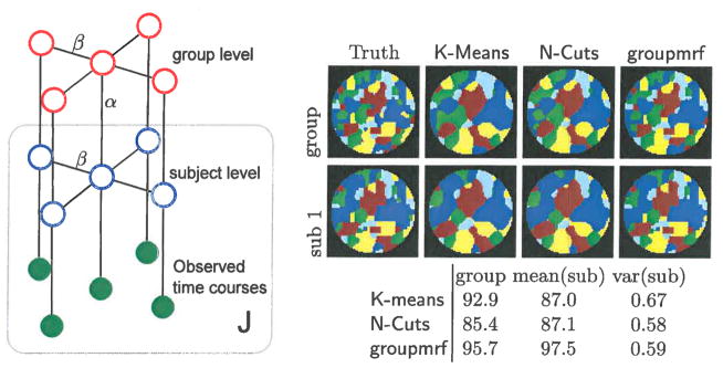
We define each subject’s network label map as a Markov Random Field (MRF) with statistical dependency between spatially adjacent voxels. These connections act as a prior model favoring spatial coherence of functional regions. An additional group label map is defined on top of all subject label maps. The group label map has the same Markov structure as the individuals, again to encourage spatial coherence of the functional regions in the group level. In addition, each voxel in the group is connected to the corresponding voxel of each subject. These connections model the relationship between the group and the individuals. Hence, all voxels of subjects and group label map are jointly connected into a single MRF. See Figure 1 for an illustration. More specifically, define a graph = ( , ), and the set of node = ( , ). is the set of voxels in the group label map, and = ( , …, ) includes voxels for all of the J subjects’ label maps. An edge (s, t) ∈ is defined if 1) s ∈ , t ∈ and s, t are at the same voxel location, or 2) if s, t ∈ , and s, t are spatial neighbors, or 3) s, t ∈ , and s, t are spatial neighbors. On each node s ∈ , a random variable y_s ∈ = {1, ···, L} is defined to represent the functional network labels.

Fig. 1.

Left: Hierarchical MRF depicted by undirected graph. The J subjects are compactly represented by a box with label J. Right: clustering of K-means and N-Cuts on synthetic time series with spatial smoothing, and groupmrf without smoothing. Top is group label map and bottom is one of subjects label map. The table gives the rand index accuracy between estimated label map and ground truth image. The rand index of all subjects are summarized by a mean and variance value.

MRF Prior

Our MRF prior on the hierarchical model is essentially a Potts model with different weights for the within-subject connections and the connections between the group and individuals. Because of the equivalence of MRFs and Gibbs fields, we define our prior as $p(Y)=\frac{1}{Z}exp\{-U(Y)\}$, where the energy function U(Y) is given by

$$U(Y)=\sum _{s,r\in \mathcal{G}}\beta \psi (y_s,y_r)+\sum _{j=1}^J\left(\sum _{s\in \mathcal{G},\stackrel{\sim }{s}\in {\mathcal{H}}^j}\alpha \psi (y_s,y_{\stackrel{\sim }{s}})+\sum _{s,r\in {\mathcal{H}}^j}\beta \psi (y_s,y_r)\right).$$

Here ψ is a binary function that is zero when the two inputs are equal and one otherwise, and α and β are parameters determining the strength of the connections. This regularization encodes two physiologically meaningful a priori assumptions on the functional networks under investigation: 1) The networks are spatially coherent within single subject. This is modeled by the β term. 2) The networks are similar between subjects, and therefore between the group and subjects. This is modeled by the α term.

Likelihood Model

In the generative model, for any individual subject, the observed time course at each voxel is assumed to be generated from a distribution conditioned on the network label at that voxel. In fMRI analysis the time series at each voxel is usually normalized to be zero mean and unit norm, so the analysis is robust to shifts or scalings of the data. This results in the data being projected onto a high-dimensional unit sphere. After normalization, the sample correlation between two time series is equal to their inner product.

We use the notation X = {(x₁, …, x_N) | x_s S^p−1} to denote the set of normalized time series in p-sphere. Given Y, the random vectors x_s are conditional independent, hence log p(X|Y) = Σ_s∈ log p(x_s|y_s). The likelihood function p(x_s|y_s) is naturally modeled by a von Mises-Fisher (vMF) distribution

$$f(x_s\mid y_s=l;{\mu }_l,{\kappa }_l)=C_p({\kappa }_l)exp\left({\kappa }_l{\mu }_l^T{x}_s\right),x_s\in S^{p-1},l\in \mathcal{L},$$ (1)

where for the cluster labeled l, μ_l is the mean direction, κ_l ≥ 0 is the concentration parameter, and C_p is the normalization constant. The larger the κ_l, the greater the density concentrated around the mean direction.

3 Bayesian Inference

We solve the inference problem in a maximum a posteriori (MAP) framework. That is, given the observed time course data X, we estimate the posterior mode of p(Y|X). This consists of the following components.

Parameter Estimation

In this data-driven model, we propose to estimate the parameters θ = {α, β, κ, μ} from the data using an Expectation Maximization (EM) algorithm. However, the high-dimensionality and dependency between spatially adjacent voxels in MRF make it infeasible to obtain a closed form solution of the expectation of [log p(X, Y)] with respect to p(Y|X). Here we propose to approximate the expectation using Monte Carlo EM (MCEM), in which a sample, (Y¹, ···, Y^M), generated from density p(Y|X) is used to approximate the expected value by the empirical average $\frac{1}{M}{\sum }_{m=1}^{M}logp(X,Y^m)$.

Gibbs Sampling

Gibbs sampling converts a multivariate sampling problem into a consecutive univariate sampling, hence is well adapted to draw the Monte Carlo samples from p(Y|X). In our hierarchical structure, the sampling procedure is also done in a hierarchical way. At the image level, a sample of the group label map, $Y_{\mathcal{G}}^m$, is drawn given the previous subject label map, $Y_{{\mathcal{H}}_j}^{m-1}$. Next, a sample for each subject map, $Y_{{\mathcal{H}}_j}^m$, is generated given the previous group label map, $Y_{\mathcal{G}}^{m-1}$. At the voxel level, we can draw samples of the label y_s given the rest of nodes fixed, and update y_s, ∀s ∈ S. The conditional probability used to generate samples at the group and subject voxels are given as

$$\begin{array}{l}p(y_s\mid y_{-s},X)\propto \frac{1}{Z_s}exp\{-U(y_s\mid y_{-s})\}·p(x_s\mid y_s)=\frac{1}{Z_s}exp\{-U_p(y_s\mid y_{{\mathcal{N}}_s},x_s)\}\\ U_p=\alpha \sum _{j=1}^J\psi (y_s,y_{\stackrel{\sim }{s}}^j)+\beta \sum _{r\in {\mathcal{N}}_s}\psi (y_s,y_r),\forall s\in \mathcal{G},\end{array}$$ (2)

$$U_p=\alpha \psi (y_s,y_{\stackrel{\sim }{s}})+\beta \sum _{r\in {\mathcal{N}}_s}\psi (y_s,y_r)-{\kappa }_l{{\mu }_l}^{\top }{x}_s-log{C}_p,\forall s\in {\mathcal{H}}_j,$$ (3)

where −s is the set of all nodes excluding s, Z_s the normalization constant, U_p is the posterior energy, and is the set of neighbor’s of s. In our model we use 6-neighbor system in a 3D volume image. $y_{\stackrel{\sim }{s}}^j$ in (2) is the label of subject j’s voxel with the same spatial location with s, and y_s̃ in (3) is the label of group’s voxel with the same spatial location with s. Because of the dependency on previous samples, the sequence of samples will be a Markov Chain, hence our method falls into Markov Chian Monte Carlo (MCMC) sampling. After a sufficient burn-in period, a series of samples Y^m, m = 1 ··· M is saved for approximating the expectation [log p(X, Y)].

Pseudo Likelihood

To evaluate log p(X, Y^m; θ) = log p(Y ^m; θ) + log p(X|Y ^m; θ) as a function of θ, we face the difficulty of evaluating the partition function Z in p(Y^m). In practice the Gibbs field is approximated by pseudo-likelihood, which is defined as the product of the conditional distribution p(y_s|y_−s), ∀s ∈ . Therefore the energy function can be written as

$$U(Y)\approx \sum _{s\in \mathcal{S}}U(y_s\mid y_{-s})=\sum _{s\in \mathcal{G}}\left(\alpha \sum _{j\in J}\psi (y_s,y_{\stackrel{\sim }{s}}^j)+\beta \sum _{r\in {\mathcal{N}}_s}\psi (y_s,y_r)\right)+\sum _{j=1}^J\sum _{s\in {\mathcal{H}}^j}\left(\alpha \psi (y_s,y_{\stackrel{\sim }{s}})+\beta \sum _{r\in {\mathcal{N}}_s}\psi (y_s,y_r)\right),$$

where $y_{\stackrel{\sim }{s}}^j$ and y_s̃ has the same definition with (2) and (3).

Hierarchical MRF Algorithm Using MCEM

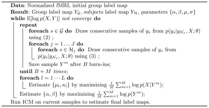
With all the preparation above, parameter estimation can be done by maximizing $\frac{1}{M}{\sum }_{m=1}^{M}logp(X,Y^m)$. The α and β in the MRF prior can be optimized by maximizing $\frac{1}{M}{\sum }_{m=1}^{M}logp(Y^m)$ with a Newton-Raphson method. We assume a Gaussian prior distribution on α with hyper-parameters μ_α and σ_α, which is given manually and does not have significant impact on the model. In order for MCMC sampling to converge quickly to the posterior, we need a reasonably good initial network label map. Here the K-means clustering on a concatenated group dataset is used for the initial maps of both the group and subjects. After the EM parameter estimation iterations are done, an Iterated Conditional Modes (ICM) on the current sample map gives the final label maps. Putting this all together, the groupmrf algorithm to estimate the group and individual label maps is given in Algorithm 1.

Algorithm 1.

Monte Carlo EM for group MRF

4 Results and Conclusion

Three methods are compared in both synthetic data and in vivo data test. The first method is K-Means [1] applied on each subject’s fMRI data, as well as on a group dataset constructed by concatenating all subjects time courses. To alleviate the dependency on initial cluster centers, we run K-Means 20 times with different initial cluster centers generated by a K-means++ algorithm. The second method is a Normalized-Cuts algorithm (N-Cuts), following Van den Heuvel, et al. [8], which is applied in two stages. First N-Cuts is run on each subject’s affinity matrix, as computed by pairwise correlation between time courses. Second, N-Cuts is applied on a group affinity matrix, which is computed by summing up all of the subjects’ segmentation matrices. We use the Ncutclustering 9 toolbox [7], a newer version of the one used in [8]. The third method is our groupmrf approach applied on all subjects’ fMRI data. The preprocessing are same for all three methods except that groupmrf use image data without spatial smoothing, while the other two use data smoothed by a standard 6mm Gaussian filter.

Synthetic Example

We simulate synthetic time course on each voxel of 16 subjects by first sampling from MRF with α = 0.4 and β = 2.0 and get both group and subjects network label map. The time course signals at each voxel are generated by adding Gaussian white noise of σ² = 40 on each cluster’s mean time course, which is synthesized from an auto-regressive process of x_t = ϕx_t−1 + ε with ϕ = 0.7 and noise variance σ_ε = 1. The sample correlation between the mean time series is in the range of (−0.15, 0.3). The rand index value on right side of Figure 1 shows that groupmrf algorithm is able to detect both group and subjects label map more accurately than the K-Means and N-Cuts method. The synthetic images shows that despite the different assumption of K-Means and N-cuts on the data, our algorithm is able to estimate subject label maps with more spatial and inter-subject coherence than the other two methods.

In Vivo Data

We tested our method on the ADHD-200 dataset in the 1000 Functional Connectomes Project. A total of 66 healthy control adolescent subjects were chosen from the same site (University of Pittsburgh). BOLD EPI images (TR = 1.5 s, TE = 29 ms, 29 slices at 4 mm slice thickness, 64 x 64 matrix, 196 volumes) were acquired on a Siemens 3 Tesla Trio scanner. The fMRI volumes were motion corrected, slice timing corrected, registered to NIHPD object 1 atlas, bandpass filtered to 0.01 to 0.1 Hz, regressed out nuisance variables including white matter, CSF mean time courses and six motion parameters, and at last filtered by a 8 mm Gaussian filter for spatial smoothness.

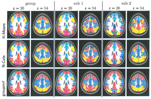
Figure 2 shows the functional networks computed from the three methods. As in the synthetic data experiment, all 66 subjects’ time series were concatenated into a single group dataset. K-means and N-Cuts were applied on the spatially-smoothed, concatenated group dataset, as well as on each subject fMRI. Our groupmrf was applied on all subjects data without any spatial smoothing and with the initial parameter values α = 0.7, β = 1.0. Following [8,1], the number of clusters are set to 7. It can be seen in Figure 2 that our algorithm is able to detect the major functional networks even for individual subjects, while K-means and N-Cuts miss some components in the Default Mode Network (DMN) for certain subjects, due to the high noise level of single subject data.

Fig. 2.

Functional networks estimated by 3 methods shown in separate rows. groupmrf has more consistent estimation of the DMN (red) and motor network (blue) among two example subjects of 66 total used.

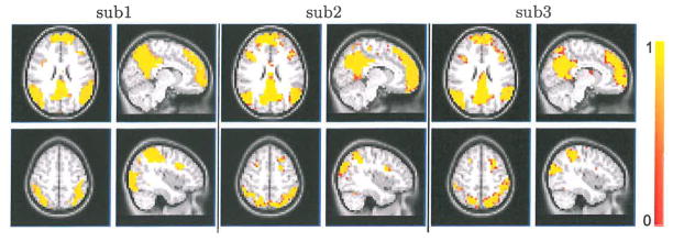
The real strength of Bayesian statistics lies in the probabilistic explanation of the results. The last experiment in Figure 3 shows the posterior probability maps of DMN and attention network of two subjects. The maps are approximated by averaging the Monte-Carlo samples from the individual posterior densities. Unlike other approaches, such as ICA or clustering, these images provide a truly probabilistic interpretation of a voxel’s membership in a particular network.

Fig. 3.

Posterior probability maps of DMN and attention network for 3 example subjects out of the 66 total used. Top row: DMN, x = −8, z = 26. Bottom row: attention network. x = 40, z = 54.

References

- 1.Bellec P, Rosa-Neto P, Lyttelton O, Benali H, Evans A. Multi-level bootstrap analysis of stable clusters in resting-state fMRI. Neuroimage. 2010;51(3):1126–1139. doi: 10.1016/j.neuroimage.2010.02.082. [DOI] [PubMed] [Google Scholar]
- 2.Calhoun V, Adali T, Pearlson G, Pekar J. Spatial and temporal independent component analysis of functional MRI data containing a pair of task-related waveforms. HBM. 2001;13(1):43–53. doi: 10.1002/hbm.1024. [DOI] [PMC free article] [PubMed] [Google Scholar]
- 3.Descombes X, Kruggel F, Von Cramon D. Spatio-temporal fMRI analysis using Markov random fields. IEEE TMI. 1998;17(6):1028–1039. doi: 10.1109/42.746636. [DOI] [PubMed] [Google Scholar]
- 4.Liu W, Zhu P, Anderson JS, Yurgelun-Todd D, Fletcher PT. Spatial Regularization of Functional Connectivity Using High-Dimensional Markov Random Fields. In: Jiang T, Navab N, Pluim JPW, Viergever MA, editors. MICCAI 2010, Part II. LNCS. Vol. 6362. Springer; Heidelberg: 2010. pp. 363–370. [DOI] [PMC free article] [PubMed] [Google Scholar]
- 5.Ng B, Abugharbieh R, Hamarneh G. CVPR 2010. IEEE; 2010. Group MRF for fMRI activation detection; pp. 2887–2894. [Google Scholar]
- 6.Ng B, McKeown M, Abugharbieh R. Group replicator dynamics: A novel group-wise evolutionary approach for sparse brain network detection. IEEE TMI. 2012;31(3):576–585. doi: 10.1109/TMI.2011.2173699. [DOI] [PubMed] [Google Scholar]
- 7.Shi J, Malik J. Normalized cuts and image segmentation. IEEE PAMI. 2000;22(8):888–905. [Google Scholar]
- 8.Van Den Heuvel M, Mandl R, Pol H. Normalized cut group clustering of resting-state FMRI data. PLoS One. 2008;3(4):e2001. doi: 10.1371/journal.pone.0002001. [DOI] [PMC free article] [PubMed] [Google Scholar]
- 9.Varoquaux G, Gramfort A, Pedregosa F, Michel V, Thirion B. Multi-subject Dictionary Learning to Segment an Atlas of Brain Spontaneous Activity. In: Székely G, Hahn HK, editors. IPMI 2011. LNCS. Vol. 6801. Springer; Heidelberg: 2011. pp. 562–573. [DOI] [PubMed] [Google Scholar]