A simple, tunable, and highly sensitive radio-frequency sensor

Abstract

We report a radio frequency (RF) sensor that exploits tunable attenuators and phase shifters to achieve high-sensitivity and broad band frequency tunability. Three frequency bands are combined to enable sensor operations from ∼20 MHz to ∼38 GHz. The effective quality factor (Q_eff) of the sensor is as high as ∼3.8 × 10⁶ with 200 μl of water samples. We also demonstrate the measurement of 2-proponal-water-solution permittivity at 0.01 mole concentration level from ∼1 GHz to ∼10 GHz. Methanol-water solution and de-ionized water are used to calibrate the RF sensor for the quantitative measurements.

Measuring the radio-frequency (RF) permittivity of materials in a microfluidic channel or nanofluidic channel is of great interest for the development of micro-total-analysis-systems (μ-TAS). The small volume and minute property changes of material-under-test (MUT) therein requires high-sensitivity RF sensors. Thus, resonator based approaches are an attractive choice, such as planar resonators,¹ resonant frequency-selective filters,² and whispering gallery mode dielectric resonators.³ Nevertheless, these sensors are limited in broadband frequency capabilities, which are needed for MUT analysis like extracting the relaxation-time of protein solutions⁴ and studying potential resonant microwave-absorptions of molecules and viruses.⁵ Additionally, current planar resonator structures have limited sensitivities since their effective quality factors, defined as Q_eff = f₀/Δf_3dB at operating frequency f₀ with a 3dB bandwidth Δf_3dB, are modest.^{1, 2} The whispering gallery mode dielectric resonators need more sophisticated fabrication and liquid handling procedures. Besides, the Q values of these devices degrade significantly when lossy MUT is introduced. Thus, it is difficult to use them to measure the properties and property changes of lossy materials.

For broadband RF sensors, such as transmission lines,⁶ tunable RF resonators,^{7, 8} harmonic-frequency/multi-mode resonators,⁹ and whispering gallery mode resonators,¹⁰ their sensitivities are limited. Further improvements are needed for challenging applications like measuring single nano-particles, viruses, and molecules in liquid.¹¹

In this work, we propose and demonstrate a simple RF sensor to simultaneously address the sensitivity and frequency tunability challenges of current techniques. The idea is based on a microwave interference process, which was first proposed and demonstrated for measuring minute dielectric property change in microfluidic channels.¹² It was later developed for single yeast cell measurements¹³ and extended for 240 GHz operations.¹⁴ Broadband performance was also reported.¹⁵ But these prior efforts have limited Q_eff and mostly operate at a single frequency point.

Figure 1a is the schematic of the proposed RF sensor. Three frequency bands are combined to cover 3-decades of operating frequencies. The detailed arrangement of band II is illustrated. Compared with the devices in Refs. ^{12, 13, 14, 15}, off-chip tuning components are introduced for continuous adjustments of phase (Φ) and attenuation (R). Broadband off-chip power dividers are also used. Band III has similar configurations. For band I, coaxial cables, instead of phase shifter Φ, are used to provide 180° phase shifts at the fundamental and certain harmonic frequency points. The yellow sensing sections are built with 50 Ω conductor-backed-coplanar-waveguides (GCPW), which are fabricated with Duroid 5870 laminates. Polydimethylsiloxane (PDMS) wells are attached to the CPWs to hold reference and MUT solutions. The dimensions of the GCPWs and PDMS wells are shown in Fig. 1b.

Figure 1.

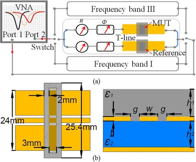
(a) A schematic of the proposed RF sensor setup. Two switches are used to combine the operations of 3 frequency-bands. Band I: from ∼20 MHz to ∼1 GHz; band II: from ∼1 to ∼12.5 GHz, and band III: from ∼26.5 to ∼38 GHz. Manual tuning components are used in this work. (b) The top view and cross section of the sensing well, where w = 2 mm, g = 1 mm, t = 17 μm, h₁ = 2.625 mm, h₂ = 0.787 mm, ε₁: MUT permittivity, ε₂: 2.33.

The sensitivity of the sensor at a given frequency f₀ is characterized by Q_eff or equivalently ${\left|S_{21}\right|}_{\min }$ if the insertion loss of the circuit components in Fig. 1a is negligible. The value of ${\left|S_{21}\right|}_{\min }$ is determined by the level of electrical balance between the two branches when reference solutions are included in the MUT and reference wells. The level of balance, i.e., the sensitivity ${\left|S_{21}\right|}_{\min }$, and the operating frequency f₀ can be tuned by the attenuators and phase shifters. The introduction of MUT or change of MUT properties will cause ${\left|S_{21}\right|}_{\min }$ and f₀ shifts, which are the sensing indicators that can be further processed to obtain MUT properties. Fig. 2 shows the measured ${\left|S_{21}\right|}_{\min }$ when de-ionized (DI) water is used as reference solutions in both wells. It shows that the RF sensor has high sensitivities over the measured frequency range. Lossy water does not significantly decrease sensor sensitivity due to its relatively small volume. This observation is further verified by doubling the PDMS well length in MUT branch. Nevertheless, the amount of water used in the tests is large in the context of μ-TAS due to large CPW dimensions. Considering the scalability of CPW sizes, the achieved ${\left|S_{21}\right|}_{\min }$ also indicates high sensitivities when measuring small-volume samples with nanometer CPWs. As a result, the sensor sensitivity compares favorably against current RF sensors, such as the planar ones in Refs. ^{1, 2}. Furthermore, the lowest ${\left|S_{21}\right|}_{\min }$ at ∼10.6 GHz yields a Q_eff of 3.8 × 10⁶, which is much higher than the un-loaded Q of dielectric resonators.³ This Q_eff is also comparable with that of the optical dielectric resonators, which have been developed for single molecule and single nano-particle measurements.¹¹ Nevertheless, Fig. 2 shows different ${\left|S_{21}\right|}_{\min }$ values, i.e., sensitivities, at different frequencies. The differences are mainly caused by the manual tuning operations of the attenuators and phase shifters. With better tuning components and better control, it is expected that ${\left|S_{21}\right|}_{\min }$ uniformity will be significantly improved across the operating frequency range.

Figure 2.

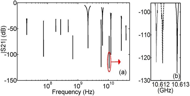
(a) Measured $\left|S_{21}\right|$ from ∼20.5 MHz to ∼38 GHz. (b) Zoom in view at one frequency point.

It should be pointed out that ${\left|S_{21}\right|}_{\min }$ values and their corresponding frequencies, f₀, fluctuate and drift with time when the RF sensor is tuned for high sensitivity operations, as shown in Fig. 2 zoom-in view. As a result, the high sensitivity tuning in Fig. 2 is only obtained for a time duration of ∼1–2 min. Such issues will be addressed in the future.

To demonstrate the process and algorithm for quantitative characterization of MUT permittivity, we use 0.01 mole fraction 2-proponal-water solutions. It is placed in the PDMS well in Fig. 1b. A plastic cylindrical tube is used to hold DI water as reference on the second and identical CPW. The use of a plastic tube is to illustrate the flexibility of the sensor. We also focus our measurements on frequency band II, from ∼1 to ∼12 GHz, where we have better tuning components as well as discrete standards for network analyzer calibration.

We intentionally tune the sensor sensitivity, ${\left|S_{21}\right|}_{\min }$, to −60 dB ∼ −70 dB level, instead of higher sensitivity operation, for a few reasons. First, the sensitivity is still very high when compared with other sensors, e.g., Refs. ^{1, 2}. It is also reasonable for measuring 2-propanol-water solutions at our targeted concentration level, which are of interest in some other efforts.¹⁶ Second, higher sensitivity would require much stricter sample handling procedures for volume and sensor stability control than simple syringe operations, which are conveniently available. Third, the relatively lower sensitivity does not affect the development of our data process algorithms.

Another issue in this effort is that our manually tunable components in Fig. 1 do not provide accurate readings. As a result, their exact phase and attenuation values are unknown. These values are also different at different frequency f₀. In order to address this issue, we assume the permittivity of water and methanol-water mixtures (at 0.01 mole fraction) are known. So, we first use water in MUT well to adjust the RF sensor at each f₀ to obtain an ${\left|S_{21}\right|}_{\min }$ of ∼−60 to ∼70 dB. Then, methanol-water mixtures are used as a standard to calibrate the sensor operation and eliminate the unknown parameters of the tuning components. Lastly, 2-propanol-water mixture is measured. Thus, three different measurements are conducted at each frequency point. Each of the 3-measurements is repeated 3-times. The obtained results are shown in Fig. 3.

Figure 3.

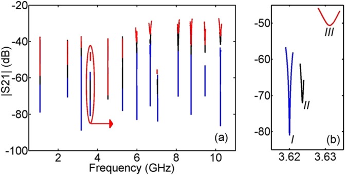
(a) The measured S₂₁ magnitude from ∼1 to ∼10 GHz for water-water, methanol-water, and 2-proponal-water solutions. (b) Zoom in view at one frequency point for DI water (I), methanol-water (II), and 2-propanol-water (III).

The following equations, obtained from analyzing signal transmission through the sensors, can be used to calculate ${\gamma }_p={\alpha }_p+j{\beta }_p$, the propagation constant of MUT section when 2-propanol-water solution is included

$$(S_{21(m)}-S_{21(w)})/(S_{21(p)}-S_{21(w)})=(\exp (-{\gamma }_{m}l)-\exp (-{\gamma }_{w}l))/(\exp (-{\gamma }_{p}l)-\exp (-{\gamma }_{w}l)),$$ (1)

where subscript m is for methanol-water solution, p for 2-propanol-water solution, and w for water-water measurement. The parameters γ_m,p,w are the corresponding propagation constants. Once ${\gamma }_p={\alpha }_p+j{\beta }_p$ is obtained, the real and imaginary permittivity components of 2-propanol-water solution, $\epsilon =\epsilon \prime -j{\epsilon }^{″}$, can be obtained through the following equations:

$$\begin{array}{c}{\alpha }_p=\pi a_1{\epsilon }_1^{″}/({\lambda }_0\sqrt{(a_0-a_1+a_1{\epsilon }_1^{\prime }+a_2{\epsilon }_2^{\prime })(a_0+a_2)})\\ {\beta }_p=2\pi f\sqrt{{\epsilon }_0{\mu }_0}\sqrt{(a_0-a_1+a_1{\epsilon }_1^{\prime }+a_2{\epsilon }_2^{\prime })/(a_0+a_2)}\end{array},$$ (2)

where parameters $a_i=2{\epsilon }_{0}K(k_i)/K(k_i^{\prime })$, i = 0,2, $a_1=2{\epsilon }_{0}K(k_1^{\prime })/K(k_1)$, K(k) is the complete elliptic integrals of the first kind with modulus k, and $k^{\prime }=\sqrt{1-k^2}$.

$$\begin{array}{c}{k}_0=w/(w+2g)\\ k_1=\sinh (\pi w/4h_1)/\sinh (\pi (w+2g)/4h_1)\\ k_2=\tanh (\pi w/4h_2)/\tanh (\pi (w+2g)/4h_2),\end{array}$$ (3)

where the geometrical parameters are defined in Fig. 1b. Fig. 4 shows the obtained permittivity of 2-proponal-water mixture. The values agree with previously published results¹⁷ reasonably well.

Figure 4.

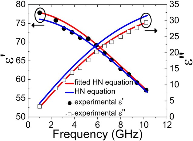
The permittivity, ε = ε′ − jε″, of 2-proponal-water mixture.

From the measured permittivity values, the relaxation time of 2-proponal-water mixtures can be obtained by fitting the Havriliak–Negami(HN) equation¹⁶

$$\epsilon (f)={\epsilon }_{\infty }+\Delta \epsilon /{(1+{(j2\pi f\tau )}^{\beta })}^{\alpha },$$ (4)

where ε_∞ is solution permittivity at infinite frequency, Δε is the permittivity change between high and low frequencies, τ is the relaxation time, and α and β are fitting constants. The obtained τ is 9.82 ps, which is close to 9.59 ps reported in Ref. 17. The rest of the parameters are ε_∞ = 8.4939 + 5.2063i, Δε = 69.7779 − 4.0773i, α = 0.99, and β = 1.0110.

The above results show that the proposed RF sensor is highly sensitive, tunable, and flexible. Different components and combinations can be used for sensing applications. Furthermore, the working principle of the sensor enables frequency scaling and size-reduction of the sensing zones. Additionally, the ultimate achievable sensor sensitivity is determined by noise that disturbs the interference process and registers at signal detectors. The noise includes phase noise of the RF signal source and noise from other system components. For high-speed operations, time-domain measurement techniques need to be developed. These issues will be addressed in our future work.

In summary, we demonstrated that the use of tunable attenuators and phase shifters for an interference-based RF sensor provides a simple and effective approach to build tunable and highly sensitive RF sensors. The obtained effective quality factors are orders of magnitude higher than that of any previously published results. Lossy materials do not significantly reduce the achievable Q values. Thus, the sensors are uniquely suited for biochemical applications. It is expected that such sensors would find wide applications in various areas, including the detection and analysis of single biological cells, particles, and molecules, electron paramagnetic resonance (EPR) spectroscopy and EPR imaging, and near field RF imaging.

References

- Chretiennot T., Dubuc D., and Grenier K., IEEE Trans. Microwave Theory Tech. 61, 972 (2013). 10.1109/TMTT.2012.2231877 [DOI] [Google Scholar]
- Costa F., Amabile C., Monorchio A., and Prati E., IEEE Microw. Wirel. Compon. Lett. 21, 273 (2011). 10.1109/LMWC.2011.2122303 [DOI] [Google Scholar]
- Shaforost E. N., Klein N., Vitusevich S. A., Barannik A. A., and Cherpak N. T., Appl. Phys. Lett. 94, 112901 (2009). 10.1063/1.3097015 [DOI] [Google Scholar]
- Basey-Fisher T. H., Hanham S. M., Andresen H., Maier S. A., Stevens M. M., Alford N. M., and Klein N., Appl. Phys. Lett. 99, 233703 (2011). 10.1063/1.3665413 [DOI] [Google Scholar]
- Liu T.-M., Chen H.-P., Wang L.-T., Wang J.-R., Luo T.-N., Chen Y.-J., Liu S.-I., and Sun C.-K., Appl. Phys. Lett. 94, 043902 (2009). 10.1063/1.3074371 [DOI] [Google Scholar]
- Booth J. C., Orloff N. D., Mateu J., Janezic M., Rinehart M., and Beall J. A., IEEE Trans. Instrum. Meas. 59, 3279 (2010). 10.1109/TIM.2010.2047141 [DOI] [Google Scholar]
- Poplavko Y. M., Prokopenko Y. V., Molchanov V. I., and Dogan A., IEEE Trans. Microwave Theory Tech. 49, 1020 (2001). 10.1109/22.925485 [DOI] [Google Scholar]
- Liu X., Katehi L. P. B., Chappell W. J., and Peroulis D., J. Microelectromech. Syst. 19, 774 (2010). 10.1109/JMEMS.2010.2055544 [DOI] [Google Scholar]
- Rowe D. J., Porch A., Barrow D. A., and Allender C. J., IEEE Trans. Microwave Theory Tech. 60, 1699 (2012). 10.1109/TMTT.2012.2189124 [DOI] [Google Scholar]
- Krupka J., Derzakowski K., Abramowicz A., Tobar M. E., and Geyer R. G., IEEE Trans. Microwave Theory Tech. 47, 752 (1999). 10.1109/22.769347 [DOI] [Google Scholar]
- Armani D. K., Kippenberg T. J., Spillane S. M., and Vahala K. J., Nature 421, 925 (2003). 10.1038/nature01371 [DOI] [PubMed] [Google Scholar]
- Song C. and Wang P., Appl. Phys. Lett. 94(2), 023901 (2009). 10.1063/1.3072806 [DOI] [Google Scholar]
- Yang Y., Zhang H., Zhu J., Wang G., Tzeng T. R., Xuan X., Huang K., and Wang P., Lab Chip 10(5), 553 (2010). 10.1039/b921502f [DOI] [PubMed] [Google Scholar]
- Wessel J., Schmalz K., Gastrock G., Cahill B. P., and Meliani C., J. Phys.: Conf. Ser. 434, 012033 (2013). 10.1088/1742-6596/434/1/012033 [DOI] [Google Scholar]
- Kozhevnikov A., Meas. Sci. Technol. 21, 043001 (2010). 10.1088/0957-0233/21/4/043001 [DOI] [Google Scholar]
- Sato T., Chiba A., and Nozaki R., J. Chem. Phys. 112, 2924 (2000). 10.1063/1.480865 [DOI] [Google Scholar]
- Sato T. and Buchner R., J. Chem. Phys. 119, 10789 (2003). 10.1063/1.1620996 [DOI] [Google Scholar]