

Abstract
Purpose: Human subjects in standing positions are apt to show much more involuntary motion than in supine positions. The authors aimed to simulate a complicated realistic lower body movement using the four-dimensional (4D) digital extended cardiac-torso (XCAT) phantom. The authors also investigated fiducial marker-based motion compensation methods in two-dimensional (2D) and three-dimensional (3D) space. The level of involuntary movement-induced artifacts and image quality improvement were investigated after applying each method.
Methods: An optical tracking system with eight cameras and seven retroreflective markers enabled us to track involuntary motion of the lower body of nine healthy subjects holding a squat position at 60° of flexion. The XCAT-based knee model was developed using the 4D XCAT phantom and the optical tracking data acquired at 120 Hz. The authors divided the lower body in the XCAT into six parts and applied unique affine transforms to each so that the motion (6 degrees of freedom) could be synchronized with the optical markers’ location at each time frame. The control points of the XCAT were tessellated into triangles and 248 projection images were created based on intersections of each ray and monochromatic absorption. The tracking data sets with the largest motion (Subject 2) and the smallest motion (Subject 5) among the nine data sets were used to animate the XCAT knee model. The authors defined eight skin control points well distributed around the knees as pseudo-fiducial markers which functioned as a reference in motion correction. Motion compensation was done in the following ways: (1) simple projection shifting in 2D, (2) deformable projection warping in 2D, and (3) rigid body warping in 3D. Graphics hardware accelerated filtered backprojection was implemented and combined with the three correction methods in order to speed up the simulation process. Correction fidelity was evaluated as a function of number of markers used (4–12) and marker distribution in three scenarios.
Results: Average optical-based translational motion for the nine subjects was 2.14 mm (±0.69 mm) and 2.29 mm (±0.63 mm) for the right and left knee, respectively. In the representative central slices of Subject 2, the authors observed 20.30%, 18.30%, and 22.02% improvements in the structural similarity (SSIM) index with 2D shifting, 2D warping, and 3D warping, respectively. The performance of 2D warping improved as the number of markers increased up to 12 while 2D shifting and 3D warping were insensitive to the number of markers used. The minimum required number of markers for 2D shifting, 2D warping, and 3D warping was 4–6, 12, and 8, respectively. An even distribution of markers over the entire field of view provided robust performance for all three correction methods.
Conclusions: The authors were able to simulate subject-specific realistic knee movement in weight-bearing positions. This study indicates that involuntary motion can seriously degrade the image quality. The proposed three methods were evaluated with the numerical knee model; 3D warping was shown to outperform the 2D methods. The methods are shown to significantly reduce motion artifacts if an appropriate marker setup is chosen.
Keywords: weight-bearing knee, C-arm cone-beam CT, XCAT, motion artifacts, fiducial marker
INTRODUCTION
Flat-panel angiography systems are suitable for assessing three-dimensional (3D) kinematics and stresses on bone and cartilage because they have high spatial resolution, good bone contrast, and highly flexible angulation. In evaluation of human subjects, the feasibility for CT reconstruction was demonstrated using a rotational angiogram in standing position, i.e., weight-bearing position.1 Novel dedicated cone-beam CT (CBCT) systems for orthopedics have also been developed to acquire weight-bearing imaging of the lower extremities.2, 3 CBCT systems with a flat panel provide superior spatial resolution with wide volumetric beam coverage along the axial direction compared to conventional CT, which allows high-resolution 3D images of entire knee in a single sweep without table translating per rotation. However, subjects in standing position are likely to show more involuntary motion than those in supine or prone positions. It is not guaranteed that the reconstructions of the standing subject data will be of diagnostic image quality. Therefore, the impact of the involuntary movements on the reconstruction image quality should be evaluated. In order to understand involuntary knee motion in weight-bearing positions, we tracked nine subjects holding a squat at 60° of knee flexion for 20 s. The subjects holding a squat position showed an average motion of about 2.4 mm at both knees, which is about 8 times larger than the detector resolution (0.308 × 0.308 mm pixel size after 2 × 2 binning) of a flat-panel angiography system.1 Since we expect greater motion in patients with knee pain, motion correction is likely required.
Two-dimensional (2D) and 3D motion compensation techniques have been developed previously. Retrospective electrocardiographic gating techniques have been implemented to reduce blurring from motion in reconstructed 3D cardiac images.4, 5, 6 Specifically, the projections corresponding to the desired cardiac phase were chosen retrospectively among the acquired projections of sometimes multiple sweeps of a C-arm. Multiple sweep acquisition requires longer acquisition time and motion estimation is available for respiratory and cardiac motions that are periodic. Moreover, inaccurate gating and imperfect periodic respiratory or cardiac motion results in residual motion blurring.7 Several studies have proposed using prior four-dimensional (4D) treatment planning CT images to acquire accurate 4D motion vector fields (MVF) or using predefined 4D MVFs.8, 9, 10, 11, 12 The results of these investigations showed fewer view-aliasing artifacts in simulated data9 compared to respiratory-correlated techniques. However, 4D deformable MVF estimation from a clinical projection image is still very difficult and computationally expensive.8 Moreover, previous CT scanning might not match well with a current scan and is sometimes difficult to acquire. Recently, an increasing number of studies have proposed novel iterative motion correction algorithms.13, 14, 15, 16, 17, 18 Iterative reconstruction first calculates the line of integrals through the initial volumetric image. Then, the forward-projected image is compared with the acquired 2D projection image. Based on the difference between them, the initial volume is updated by backward-projection as many times as necessary.13 Although iterative methods provide a higher signal-to-noise ratio (SNR) compared to the analytical reconstruction algorithms,19, 20 they are sometimes impractical due to high computational costs with relatively longer reconstruction times. Several studies have proposed either internal or external fiducial markers to track subjects’ motion.21, 22, 23, 24, 25 Fiducial marker-based methods are advantageous because they do not require additional scanning such as multiple sweeps or a prior CT scan, so there is no additional dose exposure to patients. Marchant et al.22 estimated the mean static 3D position for each marker by identifying its coordinates in multiple projections and applying the exact thin plate spline (TPS) mapping26 to warp projection images before reconstruction. The estimated static 3D position serves as a reference to correct temporal motion. It has been shown that the method does not perform well for overlaying objects with different motion in a 2D projection image. In this study, as an extension to the 2D projection warping method in Marchant et al.,22 we use the approximate TPS mapping27 to prevent unrealistic warping due to the noise in the marker locations. An alternative method, the 2D projection shifting method of Ali and Ahmad23 does not use a well-defined global reference. We adapted this method to use the estimated static 3D marker positions as a reference. Since marker locations in 2D projection images do not accurately represent their genuine location in 3D, especially in cases with different depths along the x-ray path, we also developed a 3D rigid-body warping method. To our knowledge, these fiducial marker-based motion correction algorithms have not previously been applied to lower body motion compensation.
A 4D knee phantom is needed to evaluate reconstruction and motion compensation methods. Current phantoms in CT are based on simple mathematical primitives.28, 29 On the one hand, the knee has a complicated movement resulting from individual six-degree-of-freedom (6DOF) motion of patella, femur, and tibia. Thus, it is very hard to define a realistic knee motion for manipulating a virtual phantom. Manufacturing mechanical motion-controlled phantoms using motors20, 22 is also challenging due to the aperiodicity of knee motion. In this study, we used the acquired optical motion tracking data of nine subjects holding a squat as an accurate representation of the human knee kinematics and successfully implemented the complex motion into the 4D extended cardiac-torso (XCAT) model.30 In the following, we will describe the reconstruction methods that are able to compensate for the motion of the knee during a standing acquisition on simulated data.
METHODS AND MATERIALS
Motion capture of a lower body
In order to animate the XCAT model in a realistic way, we captured a healthy volunteer's lower body movement using an eight-camera Vicon optical motion capture system (Vicon, Oxford, UK) and seven retroreflective markers while squatting at 60° of knee flexion. Three markers were attached on the sacrum (SACR), the right- and left-anterior superior iliac spine (R.ASIS and L.ASIS) to track the pelvis movement as shown in Fig. 1. Four markers were attached to the right- and left-lateral epicondyle of the knee (R.KNE and L.KNE) and the right- and left-malleolus lateralis (R.ANK and L.ANK) to track the lower extremities. The marker positions in three dimensions were recorded at a rate of 120 Hz and smoothed using a second-order low-pass Butterworth filter with a cutoff frequency of 6 Hz in order to filter out photogrammetric measurement errors from the real human involuntary motion.
Figure 1.

Seven markers (small circles on the body) were suitably placed to track a lower body. Six joint centers (big circles in the body) were estimated from the markers. Figure generated using OpenSim available on Simtk.org.
The functional right- and left-hip joint center (R.HJC and L.HJC) were estimated using a regression formula31 and SACR, R.ASIS, and L.ASIS. The right- and left-knee joint centers (R.KJC and L.KJC) were defined as the midpoint between the medial and lateral femoral epicondyles and approximated using R.KNE and L.KNE. The right- and left-ankle joint centers (R.AJC and L.AJC) were defined as the midpoint between the medial and lateral malleoli of the tibia and approximated using R.ANK and L.ANK.
The resulting tracking data of nine subjects holding a squat at about 60° of knee flexion for 20 s are shown in Table 1. In order to quantify the magnitude of the lower body motion, we calculated the translational deviation of R/L.KJC and the squatting angle (flexion) deviation as indicated in Fig. 1. Lateral knee motion along the Y-axis and flexion about the Y-axis dominated translational deviation and flexional deviation, respectively. Among the nine subjects, Subject 2 showed the largest motion in terms of translation and flexion; these data will be used to animate the model since it represents the worst case scenario. The Subject 5 data with the smallest motion will be used to represent a subject with minor motion.
Table 1.
Results of the involuntary movement at the right and left knee of nine healthy subjects while standing in a 60° position. In general, Subject 2 and Subject 5 (indicated in bold face) showed the largest and the smallest motion, respectively.
| Right knee deviation |
Left knee deviation |
|||||||
|---|---|---|---|---|---|---|---|---|
| Translation (mm) |
Flexion (deg) |
Translation (mm) |
Flexion (deg) |
|||||
| Mean | Max | Mean | Max | Mean | Max | Mean | Max | |
| Subject 1 | 2.0335 | 4.9470 | 0.6529 | 1.4243 | 2.1952 | 6.4104 | 0.6970 | 1.8155 |
| Subject 2 (largest) | 3.1735 | 12.0740 | 0.6758 | 2.1538 | 3.6851 | 12.7455 | 0.5908 | 1.7939 |
| Subject 3 | 3.3414 | 6.5166 | 0.8406 | 1.7762 | 1.4478 | 4.9131 | 0.8381 | 1.6329 |
| Subject 4 | 1.7856 | 3.4351 | 0.4677 | 1.6745 | 2.4477 | 5.5710 | 0.3932 | 0.9036 |
| Subject 5 (smallest) | 1.6426 | 5.4937 | 0.2657 | 0.6736 | 2.0744 | 5.6992 | 0.3087 | 0.9186 |
| Subject 6 | 1.3605 | 5.4032 | 0.3668 | 1.0102 | 1.9260 | 5.9417 | 0.3557 | 1.0119 |
| Subject 7 | 1.6972 | 3.6773 | 0.4050 | 0.9777 | 1.8435 | 4.5844 | 0.3330 | 0.6978 |
| Subject 8 | 2.3376 | 7.5767 | 0.4139 | 1.0475 | 2.6664 | 6.4644 | 0.4317 | 1.0034 |
| Subject 9 | 1.9283 | 5.5196 | 0.4449 | 1.1570 | 2.3398 | 6.6324 | 0.3869 | 1.2416 |
| All subjects | 2.1445 | 12.0740 | 0.5037 | 2.1538 | 2.2918 | 12.7455 | 0.4817 | 1.8155 |
Affine transformation of the XCAT knee model
The anatomical structure of the knee model is based on the surface data that is provided with the XCAT phantom. The outline of the XCAT NURBS surface is determined based on the location of its control points. Thus, we manipulated the control points to generate a 6DOF (three rotations and three translations) subject-specific knee joint model and synchronized its motion to the volunteer's motion represented by the location of the optical markers. The XCAT model was segmented into the upper leg and the lower leg. The upper leg is the part above the knee from KJC to HJC including the patella. The lower leg is the part below the knee from AJC to KJC. The two parts of each leg were animated individually using an affine transformation matrix constructed using a series of translations, scaling, and rotations in homogenous space. The patella was transformed one more time due to its distinct movement separate from that of the upper leg. The six joint center points (R/L.HJC, R/L.KJC, and R/L.AJC) in the XCAT phantom were manually identified. We defined two affine transformation matrices to map the vector () from KJC to HJC in the XCAT onto the vector () from KJC to HJC estimated from the markers and to map the vector () from AJC to KJC in XCAT onto the vector () from AJC to KJC from the markers for the upper leg and the lower leg, respectively.
For the case of the right upper leg, its transformation in homogenous space was done in seven steps using and as shown in Fig. 2. Here, represents the vector at the step n and is a homogenous vector at step (1) before transformation. Vector was translated to the origin using a translation matrix T1 so that starts from the origin. Then, was rotated to have the same direction as while maintaining its starting point at the origin using a rotational matrix R1. Now, was scaled to have the same length as using a scaling matrix S. Vector was rotated about itself to properly position the patella relative to patient front using a rotation matrix R2. Vector was translated to so that is equal to using a translation matrix T2. Finally, the patella was rotated about the vector from R.KJC to L.KJC from the markers using a rotational matrix R3. The magnitude of the rotation angle for the patella was determined by its relationship to the flexion–extension angle for the knee:32
| (1) |
| (2) |
This process is repeated at 248 different time frames for the Vicon system, synchronized to the acquisition rate of the 8 s scanning protocol used by the C-arm CT system.
Figure 2.

Transformation procedures to map onto in the upper leg. The same steps were used to transform onto in the lower leg except for step (7). The vectors are labeled with (1)–(7) representing each step. The vectors were transformed to the next step using a translation matrix T, a rotation matrix R, and a scaling matrix S.
Rendering and projection generation of the knee model
The knee is one of the pivotal hinge joints in our body. In our model, the upper leg and the lower leg were rigidly transformed individually with R/L.KJC as a pivotal hinge point. Thus, the NURBS control points in the upper leg located close to the pivot point may collide or overlap with other control points in the lower leg, leading to unrealistic wrinkle or discontinuity of body soft tissue as shown in Fig. 3a. Weighting based on the proximity to the joint was applied to body soft tissue deformation in order to avoid unrealistic wrinkles in the acute angle of the joint. To explain the description in a mathematical manner, we defined Mupper and Mlower as affine transformation matrices for the upper leg and lower leg, respectively. The weighting factor is defined to apply both Mupper and Mlower to control points, but differently depending on their proximity to the pivot point:
| (3) |
where z is the z-coordinate of the control point of interest, and zupper limit and zlower limit are the upper and lower boundary in z, respectively, where the weighting factor takes effect. For our model, we put 70 mm for the value of zupper limit and zlower limit.The final location of the control point () is determined as
| (4) |
where is the initial location of the control point in x, y, z coordinates. The proposed simple weighting method effectively eliminated the unrealistic shape of the NURBS surface in the vicinity of the pivot point in a computationally inexpensive way. Note that the XCAT model becomes subject-dependent after this transformation with respect to motion and patient size, as the correct length of the upper and lower legs are supplied to the algorithm.
Figure 3.

The XCAT knee model was tessellated and rendered as shown in (b). To avoid unrealistic wrinkles in the acute angle of the joint as shown in the windowed region in (a), weighting based on the proximity to the joint was applied.
For the generation of projections at a certain point in time, the XCAT knee model was tessellated to triangles according to the transformed control points . The XCAT knee model consists of three relevant materials: bone, bone marrow, and body soft tissue. For each detector element, all intersections with the model were determined and a monochromatic absorption model was evaluated. In total 248 views with a resolution of 620 × 480 and a pixel spacing of 0.61 mm in [u, v] were generated (Fig. 4). We assumed 70 keV of monochromatic beam energy for projection generation. As we were only interested in the motion and the respective artifact, we did not add noise. The source to detector distance was 1198 mm and the source to patient distance 780 mm. The angular increment between each projection was 0.8°. A detailed description of the rendering process is given in Maier et al.33
Figure 4.

Based on ray casting, 248 Projections with a pixel resolution of 620 × 480 were generated. Two projection views through the volume (AP and oblique) are shown.
Motion compensated reconstruction
We chose different configurations of control points on the skin around each knee in XCAT and used them as pseudo-fiducial markers. In the following this will be referred to as a marker. The markers’ position in 3D at the first time frame was defined as a reference, to correct for time-dependent motion of the lower body, where the subscript i is the marker number. The forward-projected reference point in a projection image is referred to as 2D reference, where the subscript j is the projection image number. Here, the marker's 3D position at all time points subsequent to the referential first frame was assumed unknown. In case of a clinical scan, the true 3D positions of the references are not available so one additional step is required to estimate the reference position in 3D.21, 34
Method 1: Simple projection shifting in 2D
Figure 5 shows a projection before and after shifting. The references (again, the markers at their 3D positions in the first time frame) were forward-projected onto a projection (+). The markers at a time corresponding to the projection were also forward-projected on to the projection (×). The means of the 2D references, and markers, were calculated as
| (5) |
| (6) |
where n is the number of markers used in the projection j. The r and m superscripts label the detector coordinates (u, v) belonging to the 2D references and markers, respectively. The differences (Δu, Δv) in 2D between the two means were calculated:
| (7) |
| (8) |
Then, the projection j was shifted by the amount of the difference (Δuj, Δvj) in the u and v directions. As a result of shifting, a thin black boundary was generated at left and bottom of the projection and exactly overlapped . Within the 248 projection images, |Δu| varies from 0 at the first projection up to a maximum of 7.9 pixels and |Δv| varies from 0 up to a maximum of 5.0 pixels.
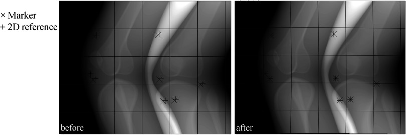
Figure 5.

A projection was shifted by the deviation (Δu, Δv) of the markers’ mean from the 2D references’ mean in a detector coordinates (u, v). The left shows the projection before shifting and the right shows the projection after shifting.
Method 2: Deformable projection warping in 2D
The projection images were warped from 2D to 2D space using the TPS.26 Figure 6 shows a projection image before and after warping in 2D. The markers and the 2D references were used as control points. The markers and the 2D references represent the original shape and the target shape, respectively. In an arbitrary projection, are the control points for the original shape and are those for the target shape where the subscript i is the number of the respective control point/marker. Deviations of from in u- and v-directions are the point loads, . Additionally, the four corner points in the projection were used as control points with zero point loads.22 Thus, the total number p of the control points was increased by four corner points. The TPS was mapped over the control points to acquire the spline interpolation function, fu(u, v) four-direction mapping first. The interpolant for the u-direction has the form:
| (9) |
We define the matrices necessary to calculate the unknown coefficients of fu(u, v) as
| (10) |
where , , , and . The control point locations could have noise especially in experimental data due to measurement error. Moreover, the control points in 2D do not accurately represent their location in 3D. This may be true even if two points appear to be close to each other in 2D; in 3D, the separation could be considerable if they are located at different depths along the x-ray path. Thus, the exact spline interpolation was relaxed by regularization parameter λ.27 The target surface did not go exactly through the control points. With the regularization parameter, the submatrices K, P, and O can be written as
| (11) |
| (12) |
| (13) |
where the subscripts i and j are the row and column number, respectively, and I is the identity matrix. As shown in Eq. 10, an inversion of a large matrix, with high condition number is necessary to compute the TPS model coefficients. In order to lower the condition number, a computationally inexpensive scaling strategy35 was adopted. In our case, the two-norm condition number of the matrix decreased roughly 14 orders of magnitude. Then, the same steps were taken to acquire the spline interpolation function, fv(u, v) for v-direction mapping with instead of .
Figure 6.
A projection was warped using approximate TPS mappings. The markers (×) were mapped smoothly onto the 2D references (+). The left and right show the projection before and after warping, respectively. The grid lines were inserted to better see overall warping of the projection.
Method 3: Rigid body warping in 3D
A 3D transformation matrix performs three rotations and three translations in x, y, and z directions in order to map references onto the identified markers. The six parameters for the matrix were optimized to minimize the distance of transformed references from the identified markers in a projection. A rotation matrix Rj and a translation matrix Tj for a projection number j were defined as
| (14) |
| (15) |
where α, β, and γ represent Euler angles using the y–x–z convention and tx, ty, and tz are translations along x, y, and z directions, respectively. Now we want to find the optimal Rj and Tj which minimize the deviation of transformed 2D references () from markers (). Again, is a 3D reference of marker number i:
| (16) |
where Pj is a projection matrix with 3 × 4 elements describing the acquisition geometry of a C-arm CT system:36
| (17) |
Optimization was done using the Nelder–Mead simplex direct search algorithm37 for every projection. While sequentially backprojecting each projection, entire voxels were transformed in 3D using the acquired Tj and Rj.
Reconstruction
Reconstructions of the projection images were performed using filtered back projection using CONRAD (A Software Framework for CONe-beam in RADiology) (Ref. 38) developed by our group. The reconstruction process was accelerated using graphics hardware (GPU),39 resulting in 512 (Ref. 3) voxels with an isotropic spacing of 0.5 mm and 32-bit depth. In case of 2D projection-based motion correction, projection images were preprocessed with the motion compensation methods before reconstruction while the 3D image warping method warped 3D images during the process of backprojection. The reconstruction pipeline consists of the following five-step sequential procedure: cosine weighting filter,40 Parker redundancy weighting filter,41 truncation correction,42 ramp filtering using Shepp–Logan ramp filter with roll-off,40 and CUDA-enabled GPU backprojection.39 A modified Shepp–Logan ramp filter with a smooth cutoff at high frequencies (cutoff frequency: 0.73 cycles/pixel, cutoff strength: 1.8) was used to suppress high frequency noise components. The frequency response of the kernel reaches its maximum at 69% of the Nyquist frequency and decreases to close to 0% at the Nyquist frequency.
Image quality metrics and investigations
For quantitative image quality comparison, we used the root-mean-square error (RSME) and the structural similarity (SSIM) index43 as image quality metrics. SSIM is an image quality metric that describes the amount of distortion in an image, compared to a gold standard, based on the degradation of structural information. Thus, if there is a structural infidelity as in our application, SSIM outperforms simple RMSE. SSIM index varies from 0 to 1, where one means that the degraded and gold standard images are identical.
We also investigated the effects of number of markers, from a minimum of six markers up to a maximum of 14, on the image quality in order to determine how many markers are needed for each motion compensation method.
Finally, the effect of marker location on correction was also investigated using eight markers. In order to determine candidate marker placements, the follow factors were considered: (i) No markers on a certain surface means that there is no information about motion in the vicinity of that surface. We assumed that a more uniform placement of markers across the field of view would provide an improved estimate of motion. (ii) We can place markers only on the skin. (iii) Markers are made of metal (tantalum) such that there is a chance that they may induce metal artifacts by photon starvation. Based on these factors, we used three different marker placement setups. The first setup, “EVEN,” evenly distributes markers across the entire skin area as shown in Fig. 8c. The second setup “TB1” evaluates evenly spaced markers placed only at the top and the bottom of the field of view. The last setup “TB2” is the same as the second one except that two markers were taken, one each from the top and bottom of the field of view and placed on the skin covering each patella.
Figure 8.

(a) and (b) An image quality comparison of motion compensated axial slice images of Subject 2 using different number of markers. The data points were interpolated using smooth cubic B-splines (the dotted lines). (c) Individual marker locations in an AP view and sequential ID number. Markers with an ID number from 1 to 11 were used for reconstruction with 11 markers.
RESULTS
The projections generated using the optical tracking data of the subject with the largest motion (Subject 2) and smallest motion (Subject 5) were reconstructed with the three different motion compensation methods. Figure 7 shows the representative reconstructed slices for Subject 2. The first column shows references reconstructed with zero motion. The first row is a central axial slice around a knee joint center and the second row is a lower axial slice containing tibia and fibula. The third row is an upper axial slice including the middle of the femoral shaft. These three slices were used to make a comparison of image quality between the three different motion compensation methods.
Figure 7.
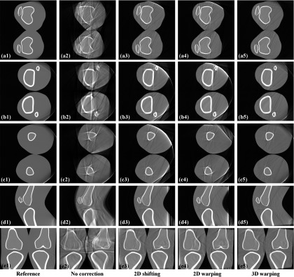
Reconstructed slices of the projections generated using the tracking data of Subject 2 with the largest motion. The first row (a) shows central axial slice and the second row (b) shows lower off-center axial slice containing tibia and fibula. The third row (c) shows upper off-center axial slice containing femur. The fourth row (d) shows sagittal slice and the fifth row (e) shows coronal slice. The slices were reconstructed with and without the motion correction methods according to the label at the bottom of each column.
Compared to the slices before motion correction shown in the second column, slices with all three different methods show fewer motion-induced artifacts. In general, 3D warping works best by showing the clearest recovered bone edge and 2D shifting and 2D warping show comparable performance in the three different axial slices (a), (b), and (c). Calculated RSME and SSIM index are shown in Table 2 below. Only the voxels in the circular field of view were included for the calculation of SSIM index and RSME.
Table 2.
Image quality comparison of Subject 2 and Subject 5 data using a different motion correction method. The “Central” is a central axial slice around a knee joint center. The “Lower” is a lower axial slice containing tibia and fibula and the “Upper” is a upper axial slice with a femoral shaft in it. The best values are reported in bold face.
| No correction |
2D shifting |
2D warping |
3D warping |
||||||
|---|---|---|---|---|---|---|---|---|---|
| Axial slice | SSIM | RSME | SSIM | RSME | SSIM | RSME | SSIM | RSME | |
| Subject 2 (largest motion) | Central | 0.4682 | 29.78 | 0.6712 | 18.70 | 0.6512 | 17.62 | 0.6884 | 17.59 |
| Lower | 0.4918 | 28.85 | 0.6457 | 17.30 | 0.6613 | 16.89 | 0.6808 | 15.05 | |
| Upper | 0.6206 | 23.56 | 0.7151 | 18.68 | 0.7165 | 18.23 | 0.7449 | 15.26 | |
| Subject 5 (smallest motion) | Central | 0.6630 | 20.28 | 0.8085 | 10.42 | 0.8305 | 8.73 | 0.7993 | 10.56 |
| Lower | 0.6630 | 25.05 | 0.8325 | 8.26 | 0.8168 | 9.61 | 0.8254 | 8.13 | |
| Upper | 0.7431 | 13.00 | 0.8013 | 9.43 | 0.8202 | 7.00 | 0.8287 | 9.17 | |
For the three axial slices of Subject 2 with the largest motion of the nine measured data sets, 3D warping outperformed (higher SSIM, lower RSME) the 2D methods as also shown qualitatively in Fig. 7. Subject 5 in Table 2 shows that a higher SSIM index does not guarantee lower RSME.43 2D shifting and 2D warping showed comparable performance over all. In the three axial slices of Subject 5, which had the smallest motion of the nine data sets, the three methods showed similar image quality improvement with a relatively higher SSIM index to begin with, compared to Subject 2. Even before motion correction in the first column, some slices show comparable image quality to the postmotion-correction slices of Subject 2.
Figure 8 shows how the image quality in terms of SSIM index changes as the number of markers used increases. Each motion correction technique responded differently to the increase of marker number. Figures 8a, 8b show that SSIM indices calculated for 2D shifting almost stay the same from marker number 6 up to 14. The SSIM index for 3D warping increases very slowly to the maximum marker number in the central slice in Fig. 8a and fluctuates initially from marker number 6 to 8 and then seems to converge around 0.70 in the lower off-center slice in Fig. 8b. The 2D warping correction shows the largest increase in SSIM index over the entire marker number range. In the central slice in (a), SSIM index for 2D warping keeps increasing until marker number 12 and then reaches a plateau and in the lower slice in (b), SSIM continues to rise with increasing number of markers although the slope of the interpolated fit line decreases as the marker number increases.
Table 3 below shows the image quality comparison between the three different marker placement setups.
Table 3.
Image quality comparison of Subject 2 using different combinations of motion correction methods and marker placement setups. As explained in Table 2, the “Central 1” and “Central 2” are representative central axial slices in the field of view. The “Lower” and “Upper” are a lower off-center axial slice and a upper off-center axial slice, respectively. The best values among different marker placement setups (“EVEN,” “TB1,” and “TB2”) with each motion correction method are reported in bold face.
| 2D shifting |
2D warping |
3D warping |
||||||||
|---|---|---|---|---|---|---|---|---|---|---|
| Axial slice | No correction | EVEN | TB1 | TB2 | EVEN | TB1 | TB2 | EVEN | TB1 | TB2 |
| Central 1 | 0.4604 | 0.6717 | 0.6766 | 0.6793 | 0.6531 | 0.6375 | 0.6481 | 0.6811 | 0.6921 | 0.6927 |
| Central 2 | 0.4795 | 0.6766 | 0.6870 | 0.6890 | 0.6598 | 0.6347 | 0.6597 | 0.6827 | 0.6992 | 0.6980 |
| Upper | 0.5743 | 0.6838 | 0.6963 | 0.6949 | 0.7028 | 0.6966 | 0.6998 | 0.7178 | 0.7209 | 0.7082 |
| Lower | 0.5048 | 0.6659 | 0.6723 | 0.6754 | 0.6286 | 0.6356 | 0.6684 | 0.7018 | 0.7076 | 0.7075 |
Each motion correction method responded differently to the three marker placement setups. In general, 2D shifting, 2D warping, and 3D warping showed best performance with the marker placement setup of TB2, EVEN, and TB1, respectively. However, the differences in the SSIM index of each marker placement setup with respect to other setups using the same motion correction method remained less than 2% (0.02) except for only 2 axial slices. The largest difference in the SSIM index was observed in the slices with 2D warping and the differences in the SSIM index between three placement setups with 2D warping were relatively larger than 2D shifting and 3D warping.
DISCUSSION
The three proposed motion correction methods in either 2D projection or 3D image space effectively reduced motion-induced artifacts. 3D warping showed better performance than the 2D methods for the data sets with relatively large motion (Subject 2 XCAT knee model). Data sets with large motion are of particular interest to us since we are planning to generate weight-bearing volumetric images of patients with an injured joint for clinical assessment and these patients are expected to show more severe involuntary motion during a scan. It is also shown in Fig. 8 that 3D warping performance was better especially in the off-center slices than in the central slice. Lateral knee motion along the Y-axis and flexion about the Y-axis dominated three translational and three rotational deviations. Due to the knee flexion about the Y-axis, the amount of motion becomes greater as the slice number moves away from the knee joint. The 2D methods performed relatively poorly since they do not incorporate rotational movements of the lower and upper leg. For the data sets with small motion (Subject 5 XCAT knee model), all the three methods showed comparable performance since rotational motion is relatively negligible. Note that we did not evaluate the area with the truncation artifacts for SSIM index and RSME.
The 2D shifting with six markers well distributed on a lower body as in (c) showed comparable performance and additional markers do not improve image quality. It is not presented here, but we confirmed that the performance of 2D shifting does not decrease even with only four markers. Thus, a marker number from 4 to 6 is adequate for 2D shifting. Image quality following correction using 2D warping improves as the number of markers increases up to 12 in the central slice. Even more markers obviously help compute the TPS model coefficients by decreasing the condition number of the large matrix, in Eq. 10 and eventually result in improved image quality. Care has to be taken not to make two or more markers overlap each other as the number of markers is increased in a projection image. We expect that it is not easy to avoid overlapping of more than 12 markers in a projection image during actual experiments and thus recommend a total of 12 markers for 2D warping. When two markers with different depth along the x-ray path are adjacent to each other or overlap in a 2D projection, unrealistic body warping around the two markers is estimated. This is because as the two markers are highly likely to have a different point load, the TPS interpolant has to enforce mapping the two adjacent markers to their 2D reference but with a large difference in point load. For that reason the exact spline interpolation was relaxed using a regularization parameter λ. 2D warping is similar to the method of Marchant et al.22 except for the regularization parameter λ. Although 3D warping with six markers has lower SSIM index than that achieved using 14 markers by 0.0115 (1.1%), we expect errors in marker location in a real scenario. We estimate that 8 markers may be required for 3D warping in order to get a stable transformation matrix. The image quality with 3D warping is better than 2D methods since the 3D correction can correct for opposite motions at different depths along the projection rays. However, it is limited in that our 3D warping assumes rigid body motion. An easy solution to this might be applying two different transformations to the upper leg and lower leg, since knee flexion is the dominant motion in the knee joint. Further extensions will be marker-less image-based motion estimation and deformable motion correction in 3D.
As shown in Table 3, 2D warping with respect to other techniques was relatively sensitive to different marker placement setups. In Central 1 and Central 2 slices with 2D warping, TB1 placement performed worst since the spline interpolant does not have motion information to fit in the central field of view and TB2 placement brought better image quality close to that with EVEN placement by providing central motion information from the marker on the patella. Therefore, an optimal marker placement setup for 2D warping is EVEN. Marker placement setups at the top and the bottom of the field of view (TB1 and TB2) showed comparable performance to the uniform marker distribution (EVEN) especially with 2D shifting and 3D warping. TB1 and TB2 setups would be a better choice than EVEN when metallic markers induce metal artifacts and thus deteriorate image quality in the central field of view. However, we did not observe serious metal artifacts from 1 mm tantalum markers in the real data scenarios.34 More practical considerations, such as overlapping markers, and markers leaving the FOV due to motion, may also limit the use of TB1 and TB2. Therefore, EVEN is a more robust choice for 2D shifting and 3D warping.
The XCAT knee model with optical tracking markers was able to simulate the complex involuntary lower body movement of the standing patient. In the optical tracking measurements of motion, some errors could potentially be introduced due to inaccurate estimation of joint centers acquired with seven retroreflective markers and a regression formula with regard to the lower body anatomy. Since we need a regression equation and three noninvasive optical markers to identify the HJC, errors of HJC location are expected to be greater than those of KJC or AJC which only requires knowledge of the medial and lateral condyles of the femur and malleoli, respectively. Stagni et al. estimated the effect of poor HJC estimation on knee joint angles and moments and showed that “the effect of HJC mislocation on knee angles and moments can be considered negligible.”44 However, even in a worst-case scenario, where errors of joint center identification become significant, the errors will not impact the amount of estimated patients’ involuntary motion since joint centers were linearly shifted in x-, y-, and z-directions. Therefore, the amount of mislocation at each time frame will be constant and consistent.
The impact of involuntary motion on image quality was estimated quantitatively and qualitatively. In vivo human subject data with the three methods show similar image quality improvement as the results of XCAT model simulation.34 Note that our XCAT model is limited as it uses a monochromatic absorption model, although we do not expect effects such as beam hardening and scatter will have a large influence on motion compensation. Moreover, the details of the soft tissues in the lower body of the XCAT phantom are lacking. Our XCAT model has only bone, bone marrow, and body soft tissue. Other tissues (e.g., cartilage, ligaments, tendon, meniscus, and muscle) are not represented in the phantom legs, which makes it hard to predict the effect of their motion on image quality. We can, however, see on the in vivo data experiments with subjects holding the squat positions that the three different motion models for the three methods are accurate enough for the amount of motion that is present in the data.34 Since the relative motion of bone and internal soft tissues (e.g., muscle, fat) to the external fiducial markers was minor, the motion compensated reconstruction based on fiducial trackers was able to visualize edges of soft tissue as well as bone. CBCT equipped with flat panels is advantageous over conventional CT in that it has high spatial resolution (e.g., 150 μm isotropic for flat-panel angiographic CT). Considering cartilage contact area45 and thickness46, 47 changes on the order of submillimeter as loads were applied, conventional CT could lead to inaccurate measurements of soft tissue structures and alignment of the bones (e.g., patella, femur, and tibia) in knee. Thus, flat panel CBCT could extract useful information of the knee joint under loading conditions which was not currently achievable. Other future work includes applying the three methods to the XCAT knee model while taking into account the impact of marker tracking errors. Tracking of multiple fiducial markers in previous studies48, 49 sometimes showed marker detection errors larger than the flat panel detector resolution in a C-arm CT system. Given marker tracking errors, the three methods show different amounts of image quality degradation.
CONCLUSIONS
The XCAT knee model with optical tracking markers was able to simulate the complex involuntary realistic lower body movement of the standing patient. The impact of involuntary motion on image quality was estimated quantitatively and qualitatively. Subjects in a squatting position showed motion amplitudes about 8 times larger than the detector resolution and thus considerable motion artifacts were observed in reconstructed images. Three different fiducial marker-based motion compensation methods (2D projection shifting, 2D projection warping, and 3D image warping) without need of prior CT scanning were developed and tested. 2D shifting, 2D warping, and 3D warping resulted in improved SSIM index by 20.30%, 18.30%, and 22.02%, respectively, in the representative central slices of Subject 2 and by 15.39%, 16.95%, and 18.90% in the representative lower off-center slices of Subject 2. As markers in 2D do not accurately represent their location in 3D, 3D image warping outperformed 2D-based methods. The three methods were also evaluated with human subject data in vivo. The suggested number of markers for 2D shifting, 2D warping, and 3D warping are 4–6, 12, and 8, respectively.
ACKNOWLEDGMENTS
This work was supported by NIH 1 R01HL087917, Siemens Medical Solutions, the Lucas Foundation, and CBIS (Center for Biomedical Imaging at Stanford) Seed Funding.
References
- Maier A., Choi J.-H., Keil A., Niebler C., Sarmiento M., Fieselmann A., Gold G., Delp S., and Fahrig R., “Analysis of vertical and horizontal circular C-arm trajectories,” Proc. SPIE 7961, 796123–796128 (2011). 10.1117/12.878502 [DOI] [Google Scholar]
- Tuominen E. K. J., Kankare J., Koskinen S. K., and Mattila K. T., “Weight-bearing CT imaging of the lower extremity,” Am. J. Roentgenol. 200(1), 146–148 (2013). 10.2214/AJR.12.8481 [DOI] [PubMed] [Google Scholar]
- Zbijewski W., De Jean P., Prakash P., Ding Y., Stayman J. W., Packard N., Senn R., Yang D., Yorkston J., Machado A., Carrino J. A., and Siewerdsen J. H., “A dedicated cone-beam CT system for musculoskeletal extremities imaging: Design, optimization, and initial performance characterization,” Med. Phys. 38(8), 4700–4713 (2011). 10.1118/1.3611039 [DOI] [PMC free article] [PubMed] [Google Scholar]
- Prümmer M., Wigstrom L., Hornegger J., Boese J., Lauritsch G., Strobel N., and Fahrig R., “Cardiac C-arm CT: Efficient motion correction for 4D-FBP,” IEEE Nucl. Sci. Symp. Conf. Rec. 4, 2620–2628 (2006). 10.1109/NSSMIC.2006.354444 [DOI] [Google Scholar]
- Lauritsch G., Boese J., Wigstrom L., Kemeth H., and Fahrig R., “Towards cardiac C-arm computed tomography,” IEEE Trans. Med. Imaging 25(7), 922–934 (2006). 10.1109/TMI.2006.876166 [DOI] [PubMed] [Google Scholar]
- Prümmer M., Hornegger J., Lauritsch G., Wigstrom L., Girard-Hughes E., and Fahrig R., “Cardiac C-arm CT: A unified framework for motion estimation and dynamic CT,” IEEE Trans. Med. Imaging 28(11), 1836–1849 (2009). 10.1109/TMI.2009.2025499 [DOI] [PubMed] [Google Scholar]
- Hansis E., Schafer D., Dossel O., and Grass M., “Projection-based motion compensation for gated coronary artery reconstruction from rotational x-ray angiograms,” Phys. Med. Biol. 53(14), 3807–3820 (2008). 10.1088/0031-9155/53/14/007 [DOI] [PubMed] [Google Scholar]
- Rit S., Wolthaus J., van Herk M., and Sonke J. J., “On-the-fly motion-compensated cone-beam CT using an a priori motion model,” Lect. Notes Comput. Sci. 5241, 729–736 (2008). 10.1007/978-3-540-85988-8_87 [DOI] [PubMed] [Google Scholar]
- Li T., Schreibmann E., Yang Y., and Xing L., “Motion correction for improved target localization with on-board cone-beam computed tomography,” Phys. Med. Biol. 51(2), 253–267 (2006). 10.1088/0031-9155/51/2/005 [DOI] [PubMed] [Google Scholar]
- Rit S., Nijkamp J., van Herk M., and Sonke J. J., “Comparative study of respiratory motion correction techniques in cone-beam computed tomography,” Radiother. Oncol. 100(3), 356–359 (2011). 10.1016/j.radonc.2011.08.018 [DOI] [PubMed] [Google Scholar]
- Blondel C., Vaillant R., Malandain G., and Ayache N., “3D tomographic reconstruction of coronary arteries using a precomputed 4D motion field,” Phys. Med. Biol. 49(11), 2197–2208 (2004). 10.1088/0031-9155/49/11/006 [DOI] [PubMed] [Google Scholar]
- Jandt U., Schafer D., Grass M., and Rasche V., “Automatic generation of time resolved motion vector fields of coronary arteries and 4D surface extraction using rotational x-ray angiography,” Phys. Med. Biol. 54(1), 45–64 (2009). 10.1088/0031-9155/54/1/004 [DOI] [PubMed] [Google Scholar]
- Isola A. A., Ziegler A., Koehler T., Niessen W. J., and Grass M., “Motion-compensated iterative cone-beam CT image reconstruction with adapted blobs as basis functions,” Phys. Med. Biol. 53(23), 6777–6797 (2008). 10.1088/0031-9155/53/23/009 [DOI] [PubMed] [Google Scholar]
- Pack J. D. and Noo F., “Dynamic computed tomography with known motion field,” Proc. SPIE 5370, 2097–2104 (2004). 10.1117/12.536283 [DOI] [Google Scholar]
- Hansis E., Schomberg H., Erhard K., Dössel O., and Grass M., “Four-dimensional cardiac reconstruction from rotational x-ray sequences: First results for 4D coronary angiography,” Proc. SPIE 7258, 72580B (2009). 10.1117/12.811104 [DOI] [Google Scholar]
- Rohkohl C., Lauritsch G., Biller L., Prümmer M., Boese J., and Hornegger J., “Interventional 4D motion estimation and reconstruction of cardiac vasculature without motion periodicity assumption,” Med. Image Anal. 14(5), 687–694 (2010). 10.1016/j.media.2010.05.003 [DOI] [PubMed] [Google Scholar]
- Wu H., Maier A., Fahrig R., and Hornegger J., “Spatial-temporal total variation regularization (STTVR) for 4D-CT reconstruction,” Proc. SPIE 8313, 83133J (2012). 10.1117/12.911162 [DOI] [Google Scholar]
- Wu H., Maier A., Hofmann H., Fahrig R., and Hornegger J., “4D-CT reconstruction using sparsity level constrained compressed sensing,” in The Second International Conference on Image Formation in X-ray Computed Tomography, Salt Lake City (2012), pp. 206–209.
- Ziegler A., Kohler T., and Proksa R., “Noise and resolution in images reconstructed with FBP and OSC algorithms for CT,” Med. Phys. 34(2), 585–598 (2007). 10.1118/1.2409481 [DOI] [PubMed] [Google Scholar]
- Rit S., Sarrut D. and Desbat L., “Comparison of analytic and algebraic methods for motion-compensated cone-beam CT reconstruction of the thorax,” IEEE Trans. Med. Imaging 28(10), 1513–1525 (2009). 10.1109/TMI.2008.2008962 [DOI] [PubMed] [Google Scholar]
- Marchant T. E., Amer A. M., and Moore C. J., “Measurement of inter and intra fraction organ motion in radiotherapy using cone beam CT projection images,” Phys. Med. Biol. 53(4), 1087–1098 (2008). 10.1088/0031-9155/53/4/018 [DOI] [PubMed] [Google Scholar]
- Marchant T. E., Price G. J., Matuszewski B. J., and Moore C. J., “Reduction of motion artefacts in on-board cone beam CT by warping of projection images,” Br J. Radiol. 84(999), 251–264 (2011). 10.1259/bjr/90983944 [DOI] [PMC free article] [PubMed] [Google Scholar]
- Ali I. and Ahmad S., “SU-GG-I-17: A technique for removing motion related image artifacts in KV cone-beam CT from on-board imager: 4D-CBCT implications,” in AAPM Annual Meeting (Medical Physics Publishing, Houston, TX, 2008), p. 2646.
- Kim J. H., Nuyts J., Kuncic Z., and Fulton R., “The feasibility of head motion tracking in helical CT: A step toward motion correction,” Med. Phys. 40(4), 041903 (4pp.) (2013). 10.1118/1.4794481 [DOI] [PubMed] [Google Scholar]
- Jacobson M. W. and Stayman J. W., “Compensating for head motion in slowly-rotating cone beam CT systems with optimization transfer based motion estimation,” IEEE Nucl. Sci. Symp. Conf. Rec. 1–9, 5240–5245 (2008). 10.1109/NSSMIC.2008.4774416 [DOI] [Google Scholar]
- Bookstein F. L., “Principal warps - thin-plate splines and the decomposition of deformations,” IEEE Trans. Pattern. Anal. 11(6), 567–585 (1989). 10.1109/34.24792 [DOI] [Google Scholar]
- Donato G. and Belongie S., “Approximate thin plate spline mappings,” Lect. Notes Comput. Sci. 2352, 21–31 (2002). 10.1007/3-540-47977-5_2 [DOI] [Google Scholar]
- Zhu J., Zhao S., Ye Y., and Wang G., “Computed tomography simulation with superquadrics,” Med. Phys. 32(10), 3136–3143 (2005). 10.1118/1.2040727 [DOI] [PubMed] [Google Scholar]
- Han E. Y., Bolch W. E., and Eckerman K. F., “Revisions to the ORNL series of adult and pediatric computational phantoms for use with the MIRD schema,” Health Phys. 90(4), 337–356 (2006). 10.1097/01.HP.0000192318.13190.c4 [DOI] [PubMed] [Google Scholar]
- Segars W. P., Sturgeon G., Mendonca S., Grimes J., and Tsui B. M., “4D XCAT phantom for multimodality imaging research,” Med. Phys. 37(9), 4902–4915 (2010). 10.1118/1.3480985 [DOI] [PMC free article] [PubMed] [Google Scholar]
- Shea K. M., Lenhoff M. W., Otis J. C., and Backus S. I., “Validation of a method for location of the hip joint center,” Gait Posture 5(2), 157–158 (1997). 10.1016/S0966-6362(97)83383-8 [DOI] [Google Scholar]
- van Eijden T. M. G. J., Kouwenhoven E., Verburg J., and Weijs W. A., “A mathematical-model of the patellofemoral joint,” J. Biomech. 19(3), 219–229 (1986). 10.1016/0021-9290(86)90154-5 [DOI] [PubMed] [Google Scholar]
- Maier A., Hofmann H. G., Schwemmer C., Hornegger J., Keil A., and Fahrig R., “Fast simulation of x-ray projections of spline-based surfaces using an append buffer,” Phys. Med. Biol. 57(19), 6193–6210 (2012). 10.1088/0031-9155/57/19/6193 [DOI] [PMC free article] [PubMed] [Google Scholar]
- Choi J. H., Keil A., Maier A., Pal S., McWalter E. J., and Fahrig R., “Fiducial marker-based motion compensation for the acquisition of 3D knee geometry under weight-bearing conditions using a C-arm CT scanner,” in AAPM 54th Annual Meeting (Medical Physics Publishing, Charlotte, NC, 2012), pp. 3973–3973. [DOI] [PubMed]
- Barrodale I., Skea D., Berkley M., Kuwahara R., and Poeckert R., “Warping digital images using thin plate splines,” Pattern Recogn. 26(2), 375–376 (1993). 10.1016/0031-3203(93)90045-X [DOI] [Google Scholar]
- Wiesent K., Barth K., Navab N., Durlak P., Brunner T., Schuetz O., and Seissler W., “Enhanced 3-D-reconstruction algorithm for C-arm systems suitable for interventional procedures,” IEEE Trans. Med. Imaging 19(5), 391–403 (2000). 10.1109/42.870250 [DOI] [PubMed] [Google Scholar]
- Lagarias J. C., Reeds J. A., Wright M. H., and Wright P. E., “Convergence properties of the Nelder-Mead simplex method in low dimensions,” SIAM J. Optim. 9(1), 112–147 (1998). 10.1137/S1052623496303470 [DOI] [Google Scholar]
- CONRAD, A software framework for cone-beam imaging in radiology, R. S. L. Stanford University School of Medicine (2013), see http://conrad.stanford.edu/. [DOI] [PMC free article] [PubMed]
- Scherl H., Keck B., Kowarschik M., and Hornegger J., “Fast GPU-based CT reconstruction using the common unified device architecture (CUDA),” IEEE Nucl. Sci. Symp. Conf. Rec. 6, 4464–4466 (2007). [Google Scholar]
- Kak A. C. and Slaney M., Principles of Computerized Tomographic Imaging (Society for Industrial and Applied Mathematics, Philadelphia, 2001). [Google Scholar]
- Parker D. L., “Optimal short scan convolution reconstruction for fan beam CT,” Med. Phys. 9(2), 254–257 (1982). 10.1118/1.595078 [DOI] [PubMed] [Google Scholar]
- Ohnesorge B., Flohr T., Schwarz K., Heiken J. P., and Bae K. T., “Efficient correction for CT image artifacts caused by objects extending outside the scan field of view,” Med. Phys. 27(1), 39–46 (2000). 10.1118/1.598855 [DOI] [PubMed] [Google Scholar]
- Wang Z., Bovik A. C., Sheikh H. R., and Simoncelli E. P., “Image quality assessment: From error visibility to structural similarity,” IEEE Trans. Image Process. 13(4), 600–612 (2004). 10.1109/TIP.2003.819861 [DOI] [PubMed] [Google Scholar]
- Stagni R., Leardini A., Cappozzo A., Benedetti M. G., and Cappello A., “Effects of hip joint centre mislocation on gait analysis results,” J. Biomech. 33(11), 1479–1487 (2000). 10.1016/S0021-9290(00)00093-2 [DOI] [PubMed] [Google Scholar]
- Bingham J. T., Papannagari R., Van de Velde S. K., Gross C., Gill T. J., Felson D. T., Rubash H. E., and Li G., “In vivo cartilage contact deformation in the healthy human tibiofemoral joint,” Br. Soc. Rheumatol. 47(11), 1622–1627 (2008). 10.1093/rheumatology/ken345 [DOI] [PMC free article] [PubMed] [Google Scholar]
- Cotofana S., Eckstein F., Wirth W., Souza R. B., Li X. J., Wyman B., Hellio-Le Graverand M. P., Link T., and Majumdar S., “In vivo measures of cartilage deformation: Patterns in healthy and osteoarthritic female knees using 3T MR imaging,” Eur. Radiol. 21(6), 1127–1135 (2011). 10.1007/s00330-011-2057-y [DOI] [PMC free article] [PubMed] [Google Scholar]
- Nishii T., Kuroda K., Matsuoka Y., Sahara T., and Yoshikawa H., “Change in knee cartilage T2 in response to mechanical loading,” J. Magn. Reson. Imaging 28(1), 175–180 (2008). 10.1002/jmri.21418 [DOI] [PubMed] [Google Scholar]
- Marchant T. E., Skalski A., and Matuszewski B. J., “Automatic tracking of implanted fiducial markers in cone beam CT projection images,” Med. Phys. 39(3), 1322–1334 (2012). 10.1118/1.3684959 [DOI] [PubMed] [Google Scholar]
- Tang X., Sharp G. C., and Jiang S. B., “Fluoroscopic tracking of multiple implanted fiducial markers using multiple object tracking,” Phys. Med. Biol. 52(14), 4081–4098 (2007). 10.1088/0031-9155/52/14/005 [DOI] [PubMed] [Google Scholar]