Model Selection in Measures of Vascular Parameters using Dynamic Contrast Enhanced MRI: Experimental and Clinical Applications

Abstract

A review of the selection of models in dynamic contrast enhanced MRI (DCE-MRI) is conducted, with emphasis on the balance between bias and variance required to produce stable and accurate estimates of vascular parameters. The vascular parameters considered as a first-order model are the forward volume transfer constant, K^trans, plasma volume fraction, v_p, and the interstitial volume fraction, v_e. To illustrate the critical issues in model selection, a data-driven selection of models in an animal model of cerebral glioma is followed. Systematic errors and extended models are considered. Studies with nested and non-nested pharmacokinetic models are reviewed; models considering water exchange are considered.

Introduction

Model selection is a prerequisite for the construction of significant inferences from relevant observations (1). In physiological studies, model selection has often been viewed as a definitive first step, to be followed by point estimation of the parameters in the model. A more data-driven approach, which we shall illustrate, describes model selection as an iterative process, with an hypothesized model as a first step, and related sub-models or extensions of the base model tested as alternatives, followed by acceptance, or reduction, or extension of the model and further testing. This paper reviews the present state of model selection in dynamic contrast enhanced MRI (DCE-MRI) studies that generally are intended to construct inferences about the physiological state of a target tissue (e.g. solid tumors). It compares some competing models, and identifies those recent efforts that show the way forward toward a stable estimate of physiological parameters obtained via DCE-MRI studies. The process we describe is data-driven; in order to demonstrate some of the central elements of data-driven model selection in DCE-MRI, particularly as they relate to sources of bias, an example from a study in a rodent model of cerebral glioma will be followed.

The Models and Their Parameters

DCE-MRI assessments are intended to allow inferences about the physiological properties of a target tissue. Vascular and tissue properties of interest might include flow per unit volume of tissue, i.e. specific flow (F), plasma volume fraction (v_p), mean transit time (t̄), the rates of transfer of contrast agent (CA) across the microvasculature, parameterized by the forward volume transfer constant (K^trans), the reverse transvascular transfer rate constant (k_ep), the permeability-surface area product (PS), extravascular extracellular volume fraction (v_e), and the diffusion constant of the indicator in the interstitial space (D_i). An updated review of pharmacokinetic models relevant to the estimate of F, v_p, t̄, K^trans, k_ep, and v_e is presented by Sourbron and Buckley in this issue. When MRI is used as an in vivo measure of indicator concentration, transvascular water exchange rate and transcytolemmal water exchange rate may affect the relationship between MRI contrast and CA concentration. Studies of water exchange in tissues as it affects measures of T₁ have a long history and a current interest in their own right (2–7). However, this review will focus on water exchange in tissues as it relates to DCE-MRI studies. Water exchange in pharmacokinetic modeling of DCE-MRI studies has been most studied in breast cancer (8–10), but there are several studies in animal models of cerebral tumor that are relevant (11–13).

Bias and Variance - Two Fundamental Concepts

Model comparisons emerge from the problem of parametric point estimation via the likelihood approach to data analysis, due originally to Fisher, and presented in most texts on mathematical statistics (14,15) or signal detection (16). The DCE-MRI experiment is an example of a stationary stochastic process (16). The voxel-by-voxel measurements of image intensity before, during, and after injection of a contrast agent are viewed as the sampling of a random variable (signal intensity) with time in a system whose physiological properties (F, v_p, K^trans, k_ep, etc.) presumably do not vary during the observation. From the point of view of likelihood theory, all of the parametric estimates we have named are functions of random variables (i.e., the DCE-MRI signal intensities), and thus also must be viewed as random variables to which the fundamental concepts of bias and variance apply.

Bias is a measure of the difference between the expected mean of an experiment that is meant to estimate the value of a parameter, and the true value of that parameter (15). An unbiased estimate of a parameter, or of a function of a parameter, is a desirable outcome because it assures that similarly unbiased estimates can be compared to one another.

Variance, often notated as ${\sigma }_{\tau \mathit{(}\theta \mathit{)}}^2$, in the estimate of a parameter τ(θ) is a measure of its dispersion around its expected mean. Thus, ${\sigma }_{\tau \mathit{(}\theta \mathit{)}}^2$ gives the investigator an idea about how close to the true value of τ(θ), on the average, one might expect to sample. It is a consequence of the Cramér-Rao inequality (14,15) that biased estimates can be expected to have lower mean-square errors (i.e. lower ‘variances’) than unbiased estimates.

In physical measurements, bias is associated with systematic errors, and variance is associated with random-like errors. Both types of error influence model choice, with random-like errors in the estimates of the parameters (and the covariances of the errors) limiting the number of parameters to be estimated, and systematic errors introducing bias into the parameters that can be estimated for a given level of signal to noise (S/N).

Systematic errors contribute to signal behavior in a predictable manner, but are not included in the model employed. Random-like errors do not contribute in a predictable manner, but introduce variance into the parametric estimates of the model. An example of a random-like error in a DCE-MRI experiment is the presence of NMR ‘white’ thermal noise in the sample and coils. Two examples of systematic behavior in a DCE-MRI experiment are the presence of $T_2^{*}$ dephasing and/or the restricted exchange of water across compartmental boundaries, with a subsequent loss of image intensity response following contrast agent (CA) administration (17–19). These two systematic behaviors are mentioned because they are often not included in the model of signal response to CA tissue concentration, and thus are potential sources of systematic error, introducing bias in estimates of the parameters that are included in the model to describe the behavior of the signal. Without some discriminant measure other than change in signal intensity after CA, it might be very difficult to distinguish between these two sources of signal loss in tissue; a model that ignores one while including the other might yield erroneous inferences.

The Principle of Parsimony

Parsimony expresses as an operating principle that a model should deploy the least number of parameters that adequately explain the phenomena being studied (1).

It is assumed that the systematic variation of the signal intensity after the administration of contrast agent can be fully parameterized, and that the fully parameterized model, or some subset of the full model, can be used to describe each data sample. Model selection addresses the question of which subset of the full model “best” describes each of the data samples of time-varying signal, with “best” defined via one of a number of related statistical and probabilistic approaches that generally deploy some measure of a cost (16) that is to be minimized.

The exclusion of a particular systematic effect from a model (i.e., the reduction of the set of parameters) will generally stabilize the estimation of the remaining parameters, but will also generate bias in their estimates. On the other hand, the inclusion of each parameter increases the variance of all parametric estimates, and the covariances of the errors in the parametric estimates. In model choice, these two costs are to be balanced. It should be noted that a probabilistic approach to model selection will not discriminate between alternative models that do not differ significantly in their goodness-of-fit. That choice must be made by comparing the usefulness of the inferences generated by the models.

Comparison of Models in DCE-MRI

Previous work has suggested that typical DCE-MRI data samples in tumor will yield three (20), or at most four (21,22), stable parametric estimates. In brain, the properties of the blood-brain barrier dictate that, in the large majority of voxels of DCE-MRI studies, K^trans and k_ep will not be different from zero. Thus, the principle of parsimony mandates that in order to make useful inferences, those parameters that are most relevant to the dynamic behavior of the data be selected and fitted.

A number of tests for comparison of alternative models have emerged. If the alternative models are nested (i.e., setting one and only one of the model parameters to zero produces a sub-model), a log-likelihood ratio test of the alternative models can be performed (14). If the alternative models are nested, and the errors of the sample are identical independently distributed and normal, an F-statistic (23) can be employed to compare model fits – this is a standard feature of most statistics packages. If the alternative models are not nested, one of a number of tests based Kullback-Leibler (24) extensions of likelihood theory can be used: the Akaike information criterion (AIC) (25,26), the Bayesian information criterion (BIC) (27), or the minimum descriptive length (MDL) (28), among others. A further description of these statistical tests is well outside the range of this review.

DCE-MRI Data in Relation to Model Selection

Because model selection should be a data-driven process, a close examination of typical data is demanded, with particular attention to sources of systematic error. As an example of DCE-MRI data, we will present an analog to human studies (20) in a DCE-MRI study at 7 Tesla in a nude rat implanted with a U251 xenograft model of cerebral glioma (29). The data demonstrates a number of systematic behaviors in a typical DCE-MRI experiment that are not accounted for in commonly used models.

The Initial Model

The full model of the time variation of signal in a DCE-MRI study should include at least F, K^trans, k_ep, v_p, and the two half-lives of water exchange (τ_b for the protons of blood, and τ_I for the intracellular water protons) – 6 free parameters in total. In the following, we will demonstrate other systematic influences on the voxel-by-voxel time variation of DCE-MRI signal. However, the contrast-to-noise ratio (CNR) usually available in DCE-MRI allows three (20), or at most four (30) model parameters. Thus, we begin with a widely used subset of the full model, the standard model (SM) of Tofts et al (31), sometimes known as the extended Tofts model. Following the initial study, we consider what additional parameters might be included in the model, given the information in the measurements.

The SM’s statement of the dependence of CA in tissue is as follows:

$$C_t\mathit{(}t\mathit{)}=K^{\mathit{\text{trans}}}\underset{0}{\overset{t}{\int }}{C}_p\mathit{(}\tau \mathit{)}{e}^{-k_{\mathit{\text{ep}}}\mathit{(}t-\tau \mathit{)}}d\tau +v_p{C}_p\mathit{(}t\mathit{)},$$ [1]

Where t is time, C_t(t) is the tissue concentration of CA, C_p(t) is the plasma concentration, K^trans is the forward volume transfer constant, k_ep is the reverse transfer rate constant, and v_p is the vascular plasma volume fraction. For a compartment diagram of this model, see Figure 9 of the review “Classic Models…” by Sourbron and Buckley in this issue. This equation is an approximation of the behavior of an indicator in tissue. The plasma fractional volume and the blood fractional volume (v_b) are related via the following: $v_b=\frac{v_p}{1-\mathit{\text{Hct}}}$, where Hct is the hematocrit of the microvasculature. The mean value of Hct in large vessels for adult human populations is about 0.45 (32). Individual deviations from that value and variation due to the Fahraeus effect (33) will affect the value of K^trans, and of v_p, proportional to the error in Hct. Thus, an unmeasured variation in microvascular hematocrit is one of the systematic factors that can bias estimates of K^trans and v_p, but one that is usually not given much weight because it is probably global in its effect.

It is a standard practice in physics and applied mathematics to state an observation equation, that is, an equation that relates observables and parameters. In DCE-MRI studies, the observation equation depends critically on the relation between CA tissue concentration and MRI contrast. In what follows, we shall assume that the change in the longitudinal relaxation rate, R₁ (R₁=1/T₁) is proportional to the total amount of CA in the tissue:

$$\mathrm{\Delta }{R}_1\mathit{(}t\mathit{)}=R_1\mathit{(}t\mathit{)}-R_1\mathit{(}0\mathit{)}={\Re }_1\mathit{\left[}Gd\mathit{\right]},$$ [2]

Where ℜ₁ is the longitudinal relaxivity of the CA in mM⁻¹sec⁻¹, and [Gd] is the tissue concentration of Gadolinium, mM. It is a requirement of our assumption of stationarity in the stochastic process that longitudinal relaxivity is assumed to be a constant. A second assumption is that longitudinal relaxivity is independent of its location in the tissue. We will revisit both assumptions when water exchange effects are discussed.

In order to proceed, we must specify a method of acquiring signal. A common tactic is to follow the change of image intensity in a saturated spoiled gradient recalled echo (SPGRE) sequence. Other sequences have been employed, e.g. various forms of a Look-Locker (LL) inversion-recovery imaging experiment (17,18,34–40).

For the SPGRE sequence, the relation between signal and R₁(t) is:

$$R_1\mathit{(}t\mathit{)}\frac{1}{TR}\mathit{\text{ln}}\lfloor \frac{1-\left(\frac{S_n\mathit{(}t\mathit{)}\mathit{\text{cos}}\mathit{(}\theta \mathit{)}}{M_0{e}^{-R_2^{*}TE}\mathit{\text{sin}}\mathit{(}\theta \mathit{)}}\right)}{1-\left(\frac{S_n\mathit{(}t\mathit{)}}{M_0{e}^{-R_2^{*}TE}\mathit{\text{sin}}\mathit{(}\theta \mathit{)}}\right)}\rfloor$$ [3]

Where: S_n(t) is the signal intensity of the n^th image in a T₁-weighted DCE-MRI procedure, t is time, M₀ is the magnetization of the protons in the voxel, θ is the local tip-angle, TR is the repetition time between pulses, TE is the echo time, and R₁(t) and R₂*(t) are the longitudinal and transverse relaxation rates in the voxel, respectively, as a function of time. When two echoes are acquired, R₂*(t) is computed as follows:

$$R_2^{*}\mathit{(}t\mathit{)}=\frac{1}{TE}\mathit{\text{ln}}\lfloor \frac{S_1\mathit{(}t\mathit{)}}{S_2\mathit{(}t\mathit{)}}\rfloor ,$$ [4]

where S₁(t) and S₂(t) are the amplitudes of first and second echoes taken at time t. M₀ which is the longitudinal equilibrium magnetization is estimated via equation 3 from R₁(0), a prior independent estimate of the longitudinal relaxation rate and S₁(0) and S₂(0), the signal prior to contrast agent injection. Thus, the relationship between ΔR₁(t) and CA tissue concentration is a fairly complex expression when expressed in terms of observables. In the following, ΔR₁(t), if fully related to observables would be expressed as ΔR₁(t,S₁(t), S₂(t), S₁(0), S₂(0), TE, TR, R₁(0), θ), with additional parameters if water exchange is considered. This is unwieldy in an observation equation, but the dependencies on observables should be noted in the following observation equation, equivalent to Equation 1:

$$\mathit{(}1-\mathit{\text{Hct}}\mathit{)}\mathrm{\Delta }{R}_{1t}\mathit{(}t\mathit{)}=K^{\mathit{\text{trans}}}\underset{0}{\overset{t}{\int }}\mathrm{\Delta }{R}_{1a}\mathit{(}\tau \mathit{)}{e}^{-k_{ep}\mathit{(}t-\tau \mathit{)}}d\tau +V_p\mathrm{\Delta }{R}_{1a}\mathit{(}t\mathit{)},$$ [5]

where R_1a is the longitudinal relaxation rate of all protons in arterial blood, and R_1t is the longitudinal relaxation rate of all protons in the tissue.

In what follows, we will not consider systematic errors in the setting of θ because in this example a previous evaluation of the tip-angle across the small extent of the brains of typical animals demonstrated that it was constant within measurement error (< 3%). However, we note without further elaboration that, in human studies tip-angle variation across the brain can vary substantially, particularly at higher fields. The systematic errors in tip-angle will then propagate into estimates of R₁(0), M₀, and ΔR₁(t), particularly at the high CA concentrations found in arterial blood, and at as the values of K^trans become large (41). Thus, some independent mapping of θ should accompany human DCE-MRI studies.

Examining the Data

To form a concrete example, let us consider a DCE-MRI experiment carried out in an athymic rat with an implanted xenograft U251 cerebral tumor at 7 Tesla. We will pay particular attention to systematic errors that are not parameterized in the observation equations, and thus are sources of bias.

The DCE-MRI study consisted of a dual-echo SPGRE (2GE) sequence with the following parameters: 150 acquisitions at 4.0 sec intervals: matrix: 128×64, three 2.0 mm slices, no gap, tip angle = 27°, NE= 2 NA=1 TE = 2.0, 4.0 ms, TR = 60 ms, SW=150 kHz. CA (0.25 mmol/kg Magnevist, Bayer Healthcare Pharmaceuticals, Wayne, New Jersey) bolus injection was performed by hand push at image 15. Total run time was 10 minutes. Prior to the DCE-MRI sequence, and immediately after, two Look-Locker (LL) sequences were run so that a voxel-by-voxel estimate of R₁(0) in the tissue could be made pre- and post-CA administration.

In this example we consider the slice that contains the largest cross-section of the tumor. Figure 1 presents a post-contrast image in the brain of the rat that will be used as an example, with an accompanying H&E-stained tissue slide approximating the position of the MR image. The tumor in both images is flame-shaped, but in the MRI, there is a prominent rim of bright contrast. This pair of images suggests that, contrary to the assumptions of the pharmacokinetic model, there may be significant transport of CA after its leakage from the vasculature of the tumor.

Figure 1.

Figure 2 shows the tissue, stained for von Willebrand factor (vessels) and counterstained with hematoxylin. A margin of (presumably leaky) new vessels surrounds the tumor mass itself. The stained vessels range in size from 100 microns downward.

Figure 2.

Figure 3 presents a set of images from the first echo (TE = 2 ms) of the 2GE sequence, numbered as to their order after the beginning of data acquisition. As a measure of S/N, signal to background was about 26:1 in the 5^th pre-contrast image. It might be expected that the major contrast change with the arrival of CA would be due to T₁ effects, demonstrated by a brightening of both vasculature and tissue with leaky microvessels. An examination of the highly vascular tissues in early images shows otherwise. Image 13 is prior to the arrival of CA, and image 14 shows the first evidence of CA in the tissue, with darkening of the blood of the sagittal sinus due to T₂* dephasing. A dark rim in and around the tumor region is evident in the next image (image 15), presumably also because of the presence of CA in the vessels feeding the tumor. The second (4 ms) echo showed even more profound decreases in image intensity. It is noticeable that the later images (e.g., image 140) showed contrast in a more extensive region than did the early images. Either the microvessels in the periphery of the tumor leaked at a slower rate than those located inward, or the streaming of tumor exudate carried CA from the leaky region of the tumor to the periphery.

Figure 3.

Figure 4 presents a time trace of the signals from the first and second echoes summed over an ROI selected in the central tumor and corresponding to the Model 3 region (see below, Figure 6). The strength of the T₂* dephasing effect is visible in the second echo of the image set, where the signal intensity shows an overall decrease in the region lasting for about 10 seconds, followed by an increase in the T₁ effect as the CA leaks out. It is evident (see Figure 2, image number 15) that, in highly vascular regions, the first echo intensity also decreases for a time.

Figure 4.

Figure 6.

Given the two echoes’ amplitudes, their echo spacing, the tip-angle of the DCE-T1 sequence, the pre-contrast amplitudes of the first and second echoes, a Look-Locker estimate of R₁(0), and the sequence repetition time, the quantities R₁(t) and R₂*(t) were calculated voxel-by-voxel using Equation 4. R₁(t) and R₂*(t) were then averaged across the tumor Model 3 region to generate the plots shown in Figure 5. It is clear that the trace of R₁(t), the best available estimate of CA tissue concentration versus time, does not follow either of the two curves of raw image contrast very well. The curve of R₂*(t) is also clearly not related to that of R₁(t), mainly because at 7 Tesla the R₂* relaxivity of the CA changes by as much as a factor of 10 as it leaks out of the microvasculature (42). It should be clear from Figures 3, 4, and 5 that T₂* dephasing is a major source of bias in the estimate of the tissue concentration-time trace of CA, and that without a measurement of the effect, no ad-hoc correction will reliably correct for T₂* dephasing. Note that, while T₂* dephasing is particularly visible at high fields, since the effect is linear in field strength (43), it is still present at the lower fields typical of clinical imaging. Thus, T₂* dephasing, almost never measured in clinical DCE-MRI studies, is a potential source of bias in DCE-MRI parametric estimates.

Figure 5.

Examining the Data: the AIF

In many prior investigations, it was noted that the arterial input function (AIF) was a dominant source of variability in the parametric estimates. For instance, Harrer et al (44) noted that two methods of estimating vascular parameters that should yield approximately equal estimates of v_p were not correlated until the estimates were scaled by their input functions. To cope with the many difficulties of actually measuring an arterial input function using T1-weighted imaging, the original Tofts model (45) employed a standardized input function, fitted to a cohort of previously measured Gd-DTPA concentration curves in healthy human volunteers (46). A reference tissue approach (47,48) has also been employed to bypass the measurement of the AIF entirely, but does not allow an estimate of the vascular volume. For slower data acquisition, and in brain, where the timing lag and dispersion between arterial and venous blood did not significantly affect the estimate of the time constants, a venous profile was utilized (35,49). In a clinical study of cerebral glioma, arterial temporal profiles were selected, and then normalized to the vasculature in normal white matter (20).

In the example we are following, a radiological (i.e. a procedure that employed radiolabeled CA) input function obtained from previous investigations (49) was adjusted in amplitude to yield a 1% plasma volume in the normal caudate putamen of the opposite hemisphere. This input function was then used as an estimate of ΔR_1a(t) in equation 2. Although it is a common practice, the use of a standardized input function, normalized to a tissue, should generate a bias in all of the parametric estimates. However, even if a good AIF could be measured at the level of the large vessels, a major artifact in the AIF is created by the dispersion of the input function as it travels through the feeding vasculature to the tissue microvessels.

Consider Figure 6. The smooth curve is an averaged arterial concentration-time curve from a group of rats studied (49) using ¹⁴C-tagged Gd-DTPA. The sampling interval of the post-peak curve varied downward in such a manner that the expected recirculation ‘bump’ was not seen, but this curve is otherwise a credible input function in large vessels. The other curve with data points marked, the tissue curve, is the curve of ΔR₁(t), gathered and averaged from the caudate putamen. It is thought that this tissue, normal brain, does not leak CA in any measurable quantity. Despite the noisiness of the tissue curve, it is clear that the two curves do not have the same shape, or timing. Consider Equations 3 and 4. If K^trans = 0, then these equations state that the tissue response is some small constant (~1%) times the arterial concentration. That is clearly not the case. There are a number of possible causes of the visible dispersion that occurs. There may in fact be some penetration of the blood-brain barrier by the CA; perhaps this small molecule penetrates the tissue of those vessels that are surrounded by smooth muscle. There is undoubtedly some dispersion in the shape of the input function that is due to the branching of the vessels between the major arteries, where the arterial input function must be sampled, and the arterioles that deliver the CA to the capillary bed of the tissue. There is dispersion in the capillary bed itself, and finally there is some restriction of water exchange (see below) between the intravascular plasma, where the CA resides, and the extravascular tissue, where the great majority of tissue water, and therefore the great majority of MRI signal, resides.

The Model and the Data

Equation 5 states a belief that, despite the effects described above, the major contributions to the time-dependent behavior of change in the longitudinal relaxation rate of the tissue are described by: 1) the filling of the vasculature with CA in the plasma; 2) the leakage of the CA from the microvasculature to the interstitial space; 3) the reflux of CA from the interstitial space to the microvasculature. These are sequential conditions: 2 cannot occur without first 1 happening, and 3 cannot occur without 2 first happening. The parameter vectors that are associated with these three conditions are v_p, v_p and K^trans, and v_p, K^trans and k_ep. We have named these three models as Model 1, Model 2, and Model 3, respectively, corresponding with the number of parameters to be estimated; note that these are physiologically and mathematically nested models. In order to cover all the possible conditions downward, we added a Model 0, in which there is insufficient evidence for filling of the vasculature with CA.

Model Selection

How are we to decide which model to select for each voxel’s data sample? In this example, as in previous work (20,36) an “extra sum of squares analysis for nested variables” (50) was employed to examine which model best described the data. An F statistic was generated that compared each of the nested models (0, 1, 2, 3), a general threshold of the F statistic for acceptance of the higher-order model was selected, and the parameters of the highest-order acceptable model were used for data summary. The fitting procedures produced, at most, maps of v_p, K^trans, k_ep, and F-tests for Model 0 vs. 1, Model 1 vs. 2, and Model 2 vs. 3 (F_0v1, F_1v2, and F_2v3, respectively). A nearly complete map of v_p (excepting only Model 0 voxels) could be produced for all MRI slices, a partial map of K^trans could be produced for those regions where evidence of leakage was sufficiently strong, and a smaller map of k_ep could be presented in those regions where there was sufficient evidence of tissue-to-vascular reflux.

Examining the Data –Model Fit and Model Failure

Figure 7 presents the result of voxel-by-voxel model selection in the animal of Figures 1 through 6. In examining Figure 7, one sees from left to right a nearly complete estimate of plasma volume, v_p, a map of K^trans in pixels where either Model 2 or Model 3 was accepted, a map of v_e, where Model 3 was accepted, and lastly a map of model choice. A summary table of parametric estimates by model region is presented in Table 1. Model 3 estimates of K^trans and v_e are in approximate agreement with those of human studies using MRI-DCE (20), or CT perfusion (51). Estimates of v_p are biased in some Model 2 regions - the yoke-shaped black rim of estimates for plasma volume in the Model 2 regions surrounding the tumor contains numerous negative values. Since a negative estimate for v_p signals a violation of mass conservation, there is clear evidence of artifact (i.e., an instance of model failure) in this region. This region coincides with the rim of bright contrast in Figure 1. The apparent cause of this model failure is the transport, via tumor exudate streaming, of the CA from interior adjacent voxels to the voxels where the negative estimates of v_p appear.

Figure 7.

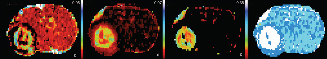
Table 1.

Parameter Summary in Regions by Model

Model 2			Model 3
Pixels	vp X10−3	Ktrans [min−1] X10−3	Pixels	vp X10−2	Ktrans [min−1] X10−2	ve X10−2
323	9.69	4.00	418	1.28	2.64	8.13

Graphing sample data and its associated model fit is an elementary step in the development of relevant inferences. Since they provide intuitive answers, graphical techniques (52–54) that generate linear fits can be powerful tools in this process. Consider Figure 8, and equations 3 and 4. DCE-MRI data can be plotted in such a manner that the data, if the model is correct, can be plotted and fitted to a straight line, the slope of which is K^trans, with intercept v_p. The ordinate of the graph is called ‘stretch time.’ In Model 2, the abscissa is calculated as $\frac{\underset{0}{\overset{t}{\int }}{C}_p\mathit{(}\tau \mathit{)}d\tau }{C_p\mathit{(}t\mathit{)}}$, and in Model 3, the abscissa is calculated as $\frac{\underset{0}{\overset{t}{\int }}{C}_p\mathit{(}\tau \mathit{)}{e}^{-k_{ep}\mathit{(}t-\tau \mathit{)}}d\tau }{C_p\mathit{(}t\mathit{)}}$, with the variable k_ep iteratively adjusted to yield a best-fit approximation of a straight line to the data. Note that, for computational purposes, linearizing the problem is unnecessary, since the optimization problem remains nonlinear (in k_ep) for Model 3 (but Murase (55) describes a linear technique for optimization). However, for the purpose of examining model choice, the practice can be invaluable.

Figure 8.

To generate the data and model fit of Figure 8, the time-varying estimates of ΔR₁(t) were summed across the 248 Model 3 voxels of the tumor (Figure 7), the radiological input function was adjusted as described (see Figure 6), and a single value of k_ep was iteratively adjusted until, when plotted as an extended Patlak Plot (36,37), the model reached a best-fit solution to the data. This procedure produced a remarkably good fit, with R²=0.997; in our experience, excellent fits of this model to DCE-MRI data in cerebral glioma are typical (20). This excellent fit generated the conclusion that, for an individual voxel, three was probably the upper limit of the number of parameters that could be estimated. However, for the summed data the fit is not perfect, and, as the residuals in this plot demonstrate, there is some additional systematic behavior in the first few minutes of tissue response that is not accounted for in the model.

Further Considerations - Extended Models

As we noted in the Introduction, model selection is iterative. We have pointed to instances where there is some systematic behavior in the tissue response not accounted for in the model. Consider the last example, of deviations from the model in the first few minutes after CA arrival. The candidates for this systematic deviation from the expected linear behavior are numerous. On the luminal side of the microvasculature, it may be that, in this particular animal, the radiological input function is not correct; it may be that the heterogeneity of the tumor in the Model 3 region changes the arrival time and shape of the input function across the regions of the tumor, and thus, while the radiological input function is approximately correct, the input function at the various tumor regions is not; in a related hypothesis, it may be that the dispersion of the arterial input function due to normal flow changes the input at the tissue level (see Figure 6); it may be that restricted water exchange in the microvasculature of the tumor changes the apparent longitudinal relaxivity of the tissue in a concentration-dependent manner (3,17,19,34,56). In the tissue, it may be that convective transport of the CA takes place at a relatively high rate, thus draining the tissue of CA and violating the model, which requires that CA, once it extravasates, is reabsorbed in the vasculature of the same voxel. All of these possibilities are plausible, and in fact may all contribute to the behavior of the signal in varying amounts. Given the demanding S/N requirements typical of adding model components to response functions with an exponential kernel (57), the likelihood that a test can be developed to discriminate between these many possible contributions appears to be remote. This leaves the investigator with a somewhat arbitrary choice that depends essentially on an assessment of the most likely main contributor to the residual behavior of the signal after the first three elements of the model have been selected. There are a number of model candidates (c.f. Sourbron and Buckley (58), Koh et al (59), or the review by Sourbron and Buckley in this issue).

In the brain, there is a strong argument for the retention of the three nested models of the SM. If the SM is to be retained, two major candidates for addition to the SM have been flow (60–64) and restricted inter-compartmental water exchange (8,10,19,34,65). (In the latter case, the estimate of v_p is often suppressed.) Since S/N is at a premium, and the heterogeneity of the tumor requires the best spatial resolution available, these two models compete.

Recent Model Selection Studies in DCE-MRI

In animal studies, model selection in an implanted cerebral glioma has been described (36); more recently, a model selection paradigm in a DCE-MRI study in patients with glioblastoma has been published (20). Interestingly, that latter study is methodologically nearly a recapitulation of an earlier work (44) that considered the same hierarchy of models, but did not submit the candidate models to formal model testing. Because there are few formal studies of model selection in DCE-MRI, this paper will consider organs other than the brain. Note, however, because of the blood-brain barrier, and the absence of lymphatic drainage in the brain, there are aspects of the vascular physiology of the brain that do not appear in other organ systems.

See the review by Sourbron and Buckley in this issue for a description, equations, and diagram of the two-compartment exchange (2CXM) and adiabatic approximation to the tissue homogeneity model (AATH) models; these model systems include flow in the model of the tissue concentration-time response. In DCE-MRI studies, when flow was added to the basic parameter set of the SM, using either the 2CXM, or the adiabatic approximation to the tissue homogeneity model (AATH), the instability of the solutions was notable. In fact, in one paper (62) that estimated flow, distribution volume, PS-product, and vascular volume in brain using the 2CXM, in the paper that modeled fitting of equivalent parameters using AATH (64), and in a paper that used AATH in DCE studies in lung (66), all four parameters were not estimated simultaneously, since “… the two-compartment model having four free parameters failed to fit the actual data obtained in vivo, as well as in the simulation (62).” Rather, some tactic was adopted that involved separately fixing the value of at least one of the parameters while varying the other three. While this jack-knifing approach did yield reasonable estimates, it should be noted that, because when one parameter is fixed, the final optimized estimates of model parameters often depend on the starting point of the fitting procedure, the final parametric estimates were likely to be biased.

In studies that summed data over an ROI drawn by a radiologist, and then fitted temporal changes in the summed data, we have studies in bladder cancers (67), and in cervical cancers (63). In both studies, since the concentration-time curve in tissue summed a presumably large number of voxels (possibly in the hundreds), S/N was enhanced to the point where all four parameters of the 2CXM model could be simultaneously estimated, and in Bains et al (67), the matter of whether water exchange was a significant contribution to the time variation of the data in this typically homogeneous tumor was also examined. In Donaldson et al (63), an F-statistic was generated for the 2CXM model versus the SM, and it was concluded that in all 30 patients studied, the 2CXM model generated significantly superior fits, as judged by the F-statistic. These were significant results, but must be tempered by the considerations stated above, in which the potential systematic effects of summed data are discussed, though the choice of bladder cancer (67) significantly ameliorates this concern.

A recent paper using models with as many as the four parameters of the 2CXM, and the reduced Akaike information criterion (AIC) for model selection on a voxel-by-voxel basis, investigated vascular parameters in the brains of patients with multiple sclerosis (30). Notable in this study was the preservation of stability in the model parameters, via parsimonious approaches to data fitting, while at the same time generating as much useful information as might be derived in each tissue. The procedures used some advanced imaging techniques, including view sharing (68) and a 24-channel receiver with an acceleration factor of 2. Temporal resolution was 2.1 s per image set, with 200 image sets acquired in 7 minutes. No S/N, or CNR figures were given for typical studies.

The Akaike weights, used in model comparison, can be thought of as estimates of the relative probability of a given model for a given data sample (1,21,22). As such, they can be used to generate probability-weighted estimates of parameters that candidate models have in common. For instance, in the example study shown above, Model 2 and Model 3 estimates of K^trans could be weighted by their relative probabilities and combined to form a multimodel estimate of the parameter K^trans.

Brix et al (21) used a measured (noisy) arterial input function and a realistic simulation produced by the MMID4 vascular model from the National Simulation Resource at the University of Washington to construct a realistic tissue response curve. The utility of Akaike weighting in constructing multimodel estimates of vascular parameters was investigated in three pharmacokinetic models - the full model with F, PS, v_p, and v_e - and two reduced models, a permeability-limited model (PS, v_p, and v_e), and a flow-limited model (F, v_p+v_e). In the simulations, it was found that there were a number of cases where, due to the conditions specified in the vascular model, the AIC chose the reduced models. Multimodel estimates of in-common parameters were found to improve the precision of their estimates. While estimates of F were found to be biased high in this study, estimates of the other parameters were approximately unbiased.

Contrary to these results, in a modeling study using the 2XCM model as the ground truth, and adding a realistic level of noise to the model response to a noise-free input function, Luypaert et al (22), explored the question of whether a multimodel estimate of 2XCM parameters would stabilize the estimates. Results were not promising, with a number of cases shown in which the reduced and full models competed for statistical power, producing “unexpected increases in the bias and/or uncertainty of the resulting parameter estimates.” The authors suggest that discrepancy between their findings and those of Brix et al (21) had to do with the level of noise added to the model curves. Some caution must be exercised in the interpretation of this study, because, unlike other examples of computer modeling of multimodel estimates, where admixtures of both higher- and lower-order models were used to construct the simulated data (1,21), the underlying simulated model in the Luypaert study was a pure 2CXM model. Nevertheless, the conclusion that the uncertainty in model selection can lead to large errors in multimodel estimates of parameters must be taken into account when considering multimodel parametric estimates as an alternative strategy to a definitive selection of one model per data set.

In most experimental results in the papers we have cited, no statement of measured S/N or CNR was included in the Results section. While noise power is not the only index of data quality, it is certainly a useful measure, and, since signal power in MRI studies is fairly well understood, noise power can be compared between studies and laboratories. A lack of information about S/N in typical experiments generates uncertainty in tradeoffs between spatial resolution, temporal resolution, and model selection; its inclusion might generate standards that real-life studies must reach before parameter sets could be trusted.

Other Models

We have presented a physiologically relevant set of nested models that has the virtue of also being mathematically nested. The 2CXM and AATH models extend this approach in a natural manner; both have the strength of allowing causal inferences as to the behavior of the system under study. Akaike weights may stabilize estimates of model parameters in vivo. However, there are other approaches to the construction of models, and to inferences drawn from the models.

George Box has famously said that “all models are wrong, but some are useful (69).” That represents something of an extremum in scientific approaches to modeling, since it undermines causality as a link between model and data. Nevertheless, this pragmatic approach has often been adopted in medical practice because the systems under study are so complex that often correlation, rather than causality can be established, and in many cases the correlation can be used to predict response. Thus, it is a widespread practice to discard the estimate of plasma volume in DCE-MRI (10,45), even though vascular filling with CA must precede any subsequent leakage. It is noted that plasma volume may be the least stable estimator of the three parameters of the SM (possibly because of restricted intra- to extra-vascular water exchange), but this does not necessarily impinge upon its importance, since it is known that increased vascular volume is a signature of tumor aggressiveness (70). Additionally, it may be that insufficient temporal resolution (71) and/or an incorrect model (63) lead to biased results in estimating plasma volume via the SM. To the best of our knowledge, no formal tests of model choice have been generated to demonstrate that the reduced model is a better choice than the model that includes v_p, although Harrer et al (44) did point out the advantage of the SM versus the original Tofts model that ignored v_p.

Other approaches have ignored reflux of indicator from the interstitium to the plasma (61,72) (as in the original Patlak approach (52)), with the result that v_e is not estimated, but v_p and possibly flow (F) are available. For a complete survey of all models presently in use for DCE-MRI modeling, see Sourbron and Buckley in this issue. Note that, for model systems that are not nested, likelihood ratio tests and F tests cannot be employed, but probabilistic tests (AIC, BIC, etc.) can be use.

Water Exchange in DCE-MRI Modeling

The longitudinal relaxation of the protons of water as they encounter paramagnetic molecules occurs at very small distances – typically nanometers. In liquids, since every proton has an equal likelihood of encountering a paramagnetic molecule in a given time interval (i.e. all protons are equivalent), the longitudinal relaxation rate of the ensemble of protons is proportional to the concentration of the paramagnetic compound. In tissue, where there are many distinct moieties, the relation between the relaxation rate and CA concentration is not so straightforward. First, there are restrictions (mainly between the microvascular endothelium and the interstitium) to the passage of CA, and an absolute exclusion of the CA from the cellular interior. Since CA is then restricted as to its location, the access of compartmentalized water molecules to the paramagnetic molecules becomes important.

In blood, although plasma and erythrocytes form separate compartments, water exchange proceeds at such high rates that the ensemble of all water protons in blood relaxes with a single exponential in nearly all conditions (73). On the other hand, in brain, it is known that significant barriers to water exchange exist across the blood: brain barrier (74). Limits to the intra- to extra-cellular (transcytolemmal) rate of water exchange may pertain also to the large volume of water (relative to that of interstitial space) that resides in intracellular compartments. Given these considerations, a minimum of three compartments of water should be considered when studying the longitudinal relaxation rate of tissue water protons.

The reader is referred to Paudyal et al (75), where an elegant summary of the compartmental modeling of water exchange in tissue using a compact matrix notation (equation 1), based on the model diagrammed in their Figure 1, is presented. This paper extends the earlier work of Li et al (19), and of Paudyal et al (76).

In the brain, it is assumed that the protons associated with tissue water can be characterized as residing in one of three following compartments: intravascular, interstitial, or intracellular with equilibrium water exchange kinetics taking place between these compartments (18,19,34,77). For modeling longitudinal relaxation rate of tissue water protons, the intercompartmental equilibrium water exchange kinetics can thus be described by a linear three-site two-exchange [3S2X] model (19).

Because of their significance in chemistry, systems in exchange have a long history of study in the NMR and MRI literature (78–81). These prior studies pertain directly to the problem of longitudinal relaxation in compartmentalized water exchange. In particular, the Bloch-McConnell equation (79) can be adapted for a system with three species and two exchange rates. The system of equations that results is a set of three linear differential equations with cross-terms in their coefficients. It is not the purpose of this review to examine the solution of these equations, and the tedious algebra associated with that solution (see Li et al (19), and Paudyal et al (13,75),), but note that, since there are three equations, there are three characteristic solutions that have the form of A_ie^−k_it, i = 1,2,3, with three values of A_i and k_i. The k_i typically differ by successive factors of 5 or more, but it is a mistake in most MR experiments with rapidly repeated sampling to assume that the higher k_i’s (shorter time constants) do not contribute to the solution (18,82). This error has been corrected in later studies (13,19,75),.

Landis et al, using a fast Look-Locker variant called PURR (83) in rat thigh muscle convincingly demonstrated the effect of transcytolemmal water exchange on the recovery of longitudinal magnetization (34). The system of equations was reduced to a two compartment model and a clever method was devised for displaying the very small differences between the fast-exchange assumption (FXL – the fast exchange limit assuming no restriction of water exchange) and the fast exchange regime (FXR – moderate restriction of water exchange). The experimental details were optimized for S/N: a homogeneous section of thigh muscle was chosen, and 64 slice-selective inversion recovery images were acquired without phase or read encoding, thus essentially summing all data in the slice. Tip-angle was kept to 6 degrees (this is an important detail, because the exchange effect is minimized at higher tip angles), and echo spacing was varied logarithmically, so that the last image was taken at 9.6 s after inversion. Given the assumption that a single tissue was being studied, sufficient data was available to detect deviation from a monoexponential recovery from inversion as CA was administered to the animal, equilibrating in the thigh muscle. A reliable finding in this investigation was that the response to CA in R₁ (R₁=1/T₁) in tissue did not follow the response in water: the apparent relaxivity of Gd-DTPA in the tissue was somewhat lower than that of Gd-DTPA in water. At high concentrations, the effect was much more noticeable, with the result that, across a range of concentrations, a nonlinearity of R₁ versus CA concentration occurred. These results were supported in brain tumor by modeling (13), but it was noted that for clinically relevant concentrations of CA, the discrepancy between an assumption of constant T₁ relaxivity (linear relation between R₁ and CA concentration) and the maximum deviation from linearity was probably too small to be detected in experiments where the tip-angle was around 20° and S/N was typically lower than 20. When considering error propagation in DCE-MRI estimates, for typical values of K^trans in cerebral glioma, the nonlinearities in T₁ relaxivity introduced errors that were generally less than 4%. On the other hand, estimates of plasma volume were expected to be underestimated by as much as 60%. These results were confirmed by experiment (12). Thus, in cerebral glioma, restricted water exchange across vascular boundaries is important to interpreting the outcome of the experiments vis-à-vis DCE estimates of plasma volume, but is not expected to generate a strong influence on either of the rate constants (K^trans and k_ep, and thus v_e) that are the typical products of DCE analysis.

In the full three-compartment model (13,19), there are five parameters that must be estimated from DCE data: v_p, K^trans, v_e, and the two rate constants of water exchange across the vascular endothelium, and the cellular cytolemma. Given the difficulty of fitting even four parameters to typical DCE data, the likelihood that five freely varied parameters might be simultaneously estimated appears remote. In general, then, approaches that include water exchange have eliminated or fixed two parameters (these are equivalent; eliminating the parameters fixes their values at zero). The two parameters usually chosen for elimination are v_p and the rate constant for water exchange across the vascular endothelium, leaving a three-parameter water exchange model (equivalently shutter-speed model, SSM) that estimates K^trans, v_e, and the mean intracellular water lifetime, τ_I (10).

A direct comparison of the SSM to the original Tofts model (v_p = 0) was undertaken in a study of DCE-MRI in 9 patients with squamous cell carcinoma of the head and neck (82). The BIC was used to select the most probable model, and a modified Monte-Carlo procedure was used to estimate the variances in estimates of model parameters. MRI procedures employed a clever scheme of interleaved radial acquisitions that allowed relatively high temporal sampling (2.5s) while preserving spatial information. The SM was also studied, but the main comparison employed a three-parameter SSM (K^trans, v_e, and τ_I, the intracellular water lifetime). In summed data, and in voxels with rapid uptake curves (but not in voxels with slower uptake curves), the SSM was selected by the BIC over the Tofts model. In a voxel-by-voxel analysis using the BIC, the SSM was superior to the Tofts model in three-quarters of the voxels of the tumor, for all 9 patients. In a separate analysis in three patients, the SM (v_p included in the model), when compared to the Tofts model, was also shown to improve the data fitbut did not explain the data as well as the SSM.

The statistical methodology of this study was quite thorough, with an appropriate test for model comparison, and a robust estimator for parametric variances. However, as we have noted, in a rapidly repeated experiment all of the eigenvalues of the SSM model need to be included when describing the signal response to a bolus of CA. The study under discussion employed a two-compartment model system but computed only one of the eigenvalues of the water exchange model, even though both eigenvalues contribute to the data response as time goes on in the experiment (13,84). A second reservation about the findings of the study is that not all plausible alternative models were included for comparison; for the rapidly filling tissue components, an appropriate comparison model would include flow, since an examination of typical data (Fig 8) suggests that flow is the obvious competing model to water exchange.

The three-parameter SSM has most successfully been applied to studies in breast tumors (9,10,85), with a recent pilot study in prostate cancer (86). MRI procedures were relatively undemanding (85): four to seven channel phased array breast coils, 13 to 41 s temporal resolution, 3 mm slice thickness, 256×128 matrix on a 20 to 24 cm² field of view. Nevertheless, when considering biopsy-confirmed malignant versus benign lesions in 89 patients, a very high positive predictive value (~98%) was generated by calculating ΔK^trans, the difference between an estimate of K^trans generated by the 3-parameter SSM and an estimate of K^trans generated by the 2-parameter Tofts model (i.e., the SM with v_p set to 0). A smaller study in prostate cancer yielded similar results. Thus, DCE estimates analyzed using the SSM yield an extremely significant inference using Box’s criterion of utility. As the authors note, biopsy is both expensive for, and traumatic to, the patients who are subjected to it, and the prospect that nearly two-thirds of the patients referred for needle biopsy can be excluded on the basis of a DCE-MRI study strongly supports the general use of this approach in screening for malignancies. Also supporting the idea that a significant component of tissue response is missing when rapidly enhancing lesions are considered is a previous study using more standard pharmacokinetic analyses that demonstrated a lower predictive value (87) than the nearly perfect positive predictive value of the parameter ΔK^trans.

However, ΔK^trans does not translate easily into causal models. What, for instance, would be inferred from a change downward in ΔK^trans after a therapeutic intervention? What therapeutic target (e.g. vascular, cellular, cell signaling) should be selected in the event that is ΔK^trans elevated, and points to a malignancy? In terms of the three parameters to be estimated, why is it allowable to eliminate plasma volume as a parameter of the model, when it is known that vascular proliferation is a sign both of malignancy and of likelihood of metastasis?

One weakness of the treatment of model selection in DCE-MRI studies is that, despite the tools to objectively select and combine models through the methods of multi-model parametric estimation (1), there are very few formal studies of alternative models that include all relevant alternatives. For instance, in the SSM breast cancer studies, no formal comparison to other three-parameter models (e.g., the three parameters of the SM, v_p, v_e, K^trans) was performed, so no judgment as to whether the three parameter SSM competitively provided the best fit to the data, versus other three parameter models, was available. A study that formally compared the SSM to the SM in the internal obdurator muscle (84) showed no advantage for the SSM. A comparison of DCE-MRI to dynamic computed tomography studies in bladder cancer using 2CXM as a model system (67) concluded that transvascular water exchange might affect the estimate of v_p, but the other parametric estimates were unaffected by either transvascular or transcytolemmal water exchange. These negative results should be viewed with some caution, because 1) the strength of water exchange effects depends on the sequence parameters, and particularly on the flip-angle employed, 2) the amount of CA in the tissue will determine the strength of the transcytolemmal water exchange effects 3) the tissue under study is an important determinant of the most useful model.

Finally, we note the increasing use of the formal tools of model selection (20–22,30,66) as a promising trend. If these tools are applied in a uniform and comprehensive manner to the matter of model selection in DCE-MRI studies, an objective selection of model, a balance of bias against variance, and thus a stable and reproducible estimate of model parameters.

Conclusion/Further Work

Model selection does not take place in a vacuum. It is preceded by a full theoretical description of the model system and an experiment designed to generate a system response that will allow model parameters to be estimated. Data-driven model selection is then followed by the generation of inferences based on stable parametric estimates.

In the DCE-MRI experiment, the full set of models that describes the system starts with a model of MRI data acquisition and image reconstruction combined with a model of signal response following the introduction of a paramagnetic compound to the vasculature of the tissue. A plethora of system properties influence the signal response - we have presented and discussed a number of influences, including T₂* dephasing, vascular leakage or the lack thereof, T₁ shortening, water exchange, R₂* relaxivity changes, dispersion due to flow, artifacts in acquiring an input function, etcetera. While it is convenient to treat the data acquisition as being partitioned, e.g. to consider the phenomena of image formation as separate from the phenomena of pharmacokinetics, the researcher should keep in mind that every system property will influence the final analysis, and thus impinge on the inferences drawn. For instance, we have noted that T₂* dephasing and/or water exchange and/or dispersion due to flow all might contribute to an initial decrease in T₁ signal response after CA administration.

We remind the reader that there is no substitute for good data acquired under an experimental design that has used a priori knowledge to minimize, or better yet measure, systematic effects that tend to confound inferences that might otherwise be drawn from the data.

Biological systems are complex and are generally characterized by “tapering” effects. For instance, in a DCE-MRI study in a tumor, a main effect across time might be the T₁ shortening due to CA leakage. Less dominant effects might be T₂* dephasing, dispersion of the input due to flow, water exchange, and so on. The experiment that gathers the data can and should be designed to weight the measured response of the system toward the effects that lead to the inferences that are of interest. For instance, T₂* effects can be minimized by shortening echo times, or can be estimated by acquiring multiple echoes in an SPGRE experiment. Water exchange effects can be minimized or emphasized by increasing or decreasing the flip angle.

Even when the experimental design has been optimized for the desired inference in a biological system with tapering systematic effects, there will still typically not be enough information in the data sample to fit the full model. This is where model selection enters. Model selection is a data driven process that is intended to ideally balance bias and variance in the analysis of a data set. The virtue of a formal process of model selection, such as we have described here, is that it generates, in some sense, the ‘best’ set of models that apply to the data.

Since a useful inference is the final product of experimentation, there are still areas in which the judgment of the investigators is paramount. If there are two models of the same order that describe the data equally well, the more useful model might well be chosen. On the other hand, causality may be a dominant concern, as in our example of physiologically nested models in the brain.

In DCE-MRI studies, clinically important inferences will eventually dominate model selection (Box’s criterion of utility). These may well vary from tissue to tissue, and from pathology to pathology; it may be that, because K^trans values are very high and flow and vascular volume are relatively small, water exchange models will be selected in breast cancer, and, because K^trans values are relatively low and flow and vascular volume are relatively high, 2CXM models will be selected in brain tumors (75).

A matter that we have not directly addressed, but is relevant to the model choice problem - the tradeoff between spatial resolution, temporal resolution, and S/N – should be resolved for common pathologies in consultation with clinicians. It may be that, in some pathologies, a more reliable picture of the physiological state of the tissue will trump a better localization of the pathology. This matter needs attention in the design of experiments, and modification as experience with the newly available physiological measures establishes their clinical relevance.

In order to ensure the stability of parametric estimates we recommend for all DCE-MRI studies that, when higher order models are to be used (3 or 4 parameters), they should be routinely tested against models of lower order. In the highest-order model systems, plausible alternative models of the same order should be tested against each other. It may be possible, given that scenario, to use a probabilistic approach to generate multimodel estimates of parameters that are common across alternate model systems. S/N figures should be stated for common sequences in order that noise power can be compared across sites, and estimates of the variances and covariances of the parametric estimates should be available.

References

- 1.Burnham KP, Anderson DR. Model Selection and Multimodel Inference: A Practical Information-Theoretic Approach. New York: Springer; 2002. p. 518. [Google Scholar]
- 2.Bacic G, Alameda JC, Jr, Iannone A, Magin RL, Swartz HM. NMR study of water exchange across the hepatocyte membrane. Magn Reson Imaging. 1989;7(4):411–416. doi: 10.1016/0730-725x(89)90490-6. [DOI] [PubMed] [Google Scholar]
- 3.Donahue KM, Burstein D, Manning WJ, Gray ML. Studies of Gd-DTPA relaxivity and proton exchange rates in tissue. Magnetic resonance in medicine : official journal of the Society of Magnetic Resonance in Medicine / Society of Magnetic Resonance in Medicine. 1994;32(1):66–76. doi: 10.1002/mrm.1910320110. [DOI] [PubMed] [Google Scholar]
- 4.Donahue KM, Weisskoff RM, Burstein D. Water diffusion and exchange as they influence contrast enhancement. J Magn Reson Imaging. 1997;7(1):102–110. doi: 10.1002/jmri.1880070114. [DOI] [PubMed] [Google Scholar]
- 5.St Lawrence KS, Lee TY. An adiabatic approximation to the tissue homogeneity model for water exchange in the brain: ITheoretical derivation. J Cereb Blood Flow Metab. 1998;18(12):1365–1377. doi: 10.1097/00004647-199812000-00011. [DOI] [PubMed] [Google Scholar]
- 6.Lu H, Golay X, Pekar JJ, Van Zijl PC. Functional magnetic resonance imaging based on changes in vascular space occupancy. Magn Reson Med. 2003;50(2):263–274. doi: 10.1002/mrm.10519. [DOI] [PubMed] [Google Scholar]
- 7.Kim YR, Tejima E, Huang S, et al. In vivo quantification of transvascular water exchange during the acute phase of permanent stroke. Magn Reson Med. 2008;60(4):813–821. doi: 10.1002/mrm.21708. [DOI] [PMC free article] [PubMed] [Google Scholar]
- 8.Yankeelov TE, Rooney WD, Huang W, et al. Evidence for shutter-speed variation in CR bolus-tracking studies of human pathology. NMR Biomed. 2005;18(3):173–185. doi: 10.1002/nbm.938. [DOI] [PubMed] [Google Scholar]
- 9.Li X, Huang W, Morris EA, et al. Dynamic NMR effects in breast cancer dynamic-contrast-enhanced MRI. Proc Natl Acad Sci U S A. 2008;105(46):17937–17942. doi: 10.1073/pnas.0804224105. [DOI] [PMC free article] [PubMed] [Google Scholar]
- 10.Huang W, Li X, Morris EA, et al. The magnetic resonance shutter speed discriminates vascular properties of malignant and benign breast tumors in vivo. Proc Natl Acad Sci U S A. 2008;105(46):17943–17948. doi: 10.1073/pnas.0711226105. [DOI] [PMC free article] [PubMed] [Google Scholar]
- 11.Pickup S, Chawla S, Poptani H. Quantitative estimation of dynamic contrast enhanced MRI parameters in rat brain gliomas using a dual surface coil system. Acad Radiol. 2009;16(3):341–350. doi: 10.1016/j.acra.2008.09.010. [DOI] [PubMed] [Google Scholar]
- 12.Li X, Rooney WD, Varallyay CG, et al. Dynamic-contrast-enhanced-MRI with extravasating contrast reagent: rat cerebral glioma blood volume determination. J Magn Reson. 2010;206(2):190–199. doi: 10.1016/j.jmr.2010.07.004. [DOI] [PMC free article] [PubMed] [Google Scholar]
- 13.Paudyal R, Bagher-Ebadian H, Nagaraja TN, Fenstermacher JD, Ewing JR. Modeling of Look-Locker estimates of the magnetic resonance imaging estimate of longitudinal relaxation rate in tissue after contrast administration. Magn Reson Med. 2011;66(5):1432–1444. doi: 10.1002/mrm.22852. [DOI] [PMC free article] [PubMed] [Google Scholar]
- 14.Wilks SS. Mathematical statistics. New York: 1962. p. 644. s. p. [Google Scholar]
- 15.Mood AMAGFDCB. Introduction to the Theory of Statistics. New York, N.Y: McGraw-Hill Book Co; 1963. [Google Scholar]
- 16.Helstrom CW. Statistical Theory of Signal Detection. Oxford: Pergamon Press; 1968. p. 470. [Google Scholar]
- 17.Landis CS, Li X, Telang FW, et al. Determination of the MRI contrast agent concentration time course in vivo following bolus injection: effect of equilibrium transcytolemmal water exchange. Magn Reson Med. 2000;44(4):563–574. doi: 10.1002/1522-2594(200010)44:4<563::aid-mrm10>3.0.co;2-#. [DOI] [PubMed] [Google Scholar]
- 18.Yankeelov TE, Rooney WD, Li X, Springer CS. Variation of the Relaxographic “Shutter-Speed” for Transcytoliemmal Water Exchange Affects the CR Bolus-Tracking Curve Shape. Magn Reson Med. 2003;50(6):1151–1169. doi: 10.1002/mrm.10624. [DOI] [PubMed] [Google Scholar]
- 19.Li X, Rooney WD, Springer CS., Jr A unified magnetic resonance imaging pharmacokinetic theory: intravascular and extracellular contrast reagents. Magnetic Resonance in Medicine. 2005;54(6):1351–1359. doi: 10.1002/mrm.20684. [DOI] [PubMed] [Google Scholar]
- 20.Bagher-Ebadian H, Jain R, Nejad-Davarani SP, et al. Model selection for DCE-T1 studies in glioblastoma. Magn Reson Med. 2012;68(1):241–251. doi: 10.1002/mrm.23211. [DOI] [PMC free article] [PubMed] [Google Scholar]
- 21.Brix G, Zwick S, Kiessling F, Griebel J. Pharmacokinetic analysis of tissue microcirculation using nested models: multimodel inference and parameter identifiability. Med Phys. 2009;36(7):2923–2933. doi: 10.1118/1.3147145. [DOI] [PMC free article] [PubMed] [Google Scholar]
- 22.Luypaert R, Ingrisch M, Sourbron S, de Mey J. The Akaike information criterion in DCE-MRI: does it improve the haemodynamic parameter estimates? Phys Med Biol. 2012;57(11):3609–3628. doi: 10.1088/0031-9155/57/11/3609. [DOI] [PubMed] [Google Scholar]
- 23.Chernoff H, Lehmann EL. The use of maximum likelihood estimates in c2 tests of goodness of fit. Ann Math statist. 1954;1(25):579–586. [Google Scholar]
- 24.Kullback S. Information theory and statistics. New York: 1959. p. 395. s. p. [Google Scholar]
- 25.Akaike H. A new look at the statistical model identification. IEEE Transaction on Automatic Control. 1974;19(6):716–723. [Google Scholar]
- 26.Akaike H. Information theory and an extension of the maximum likelihood principle. In: Kiado Ae., editor. 2nd International Symposium on Information Theory. Volume 1. Budapest: Information Theory; 1973. pp. 267–281. [Google Scholar]
- 27.Schwarz G. Estimating the Dimension of a Model. Annals of Statistics. 1978;6:461–464. [Google Scholar]
- 28.Grunwald PD, Myung IJ, Pitt MA. Advances in minimum description length : theory and applications. x. Cambridge, Mass: MIT Press; 2005. p. 444. [Google Scholar]
- 29.Mikkelsen T, Brodie C, Finniss S, et al. Radiation sensitization of glioblastoma by cilengitide has unanticipated schedule-dependency. Int J Cancer. 2009;124(11):2719–2727. doi: 10.1002/ijc.24240. [DOI] [PubMed] [Google Scholar]
- 30.Ingrisch M, Sourbron S, Morhard D, et al. Quantification of perfusion and permeability in multiple sclerosis: dynamic contrast-enhanced MRI in 3D at 3T. Invest Radiol. 2012;47(4):252–258. doi: 10.1097/RLI.0b013e31823bfc97. [DOI] [PubMed] [Google Scholar]
- 31.Tofts PS, Brix G, Buckley DL, et al. Estimating kinetic parameters from dynamic contrast-enhanced T(1)-weighted MRI of a diffusable tracer: standardized quantities and symbols. J Magn Reson Imaging. 1999;10(3):223–232. doi: 10.1002/(sici)1522-2586(199909)10:3<223::aid-jmri2>3.0.co;2-s. [DOI] [PubMed] [Google Scholar]
- 32.Dittmer DS. Blood and Other Body Fluids. In: Handbooks CoB., editor. Biological Handbooks. 1 ed. Washington. D.C.: Federation of American Societies for Experimental Biology; 1963. p. 540. [Google Scholar]
- 33.Fahraeus R, LIndqvist T. The Viscosity of the Blood in Narrow Capillary Tubes. American Journal of Physiology. 1931;96:562–568. [Google Scholar]
- 34.Landis CS, Li X, Telang FW, et al. Equilibrium Transcytolemmal Water-Exchange Kinetics in Skeletal Muscle In Vivo. Magnetic Resonance in Medicine. 1999;42:467–478. doi: 10.1002/(sici)1522-2594(199909)42:3<467::aid-mrm9>3.0.co;2-0. [DOI] [PubMed] [Google Scholar]
- 35.Ewing JR, Knight RA, Nagaraja TN, et al. Patlak plots of Gd-DTPA MRI data yield blood-brain transfer constants concordant with those of 14C-sucrose in areas of blood-brain opening. Magn Reson Med. 2003;50(2):283–292. doi: 10.1002/mrm.10524. [DOI] [PubMed] [Google Scholar]
- 36.Ewing JR, Brown SL, Lu M, et al. Model selection in magnetic resonance imaging measurements of vascular permeability: Gadomer in a 9L model of rat cerebral tumor. J Cereb Blood Flow Metab. 2006;26(3):310–320. doi: 10.1038/sj.jcbfm.9600189. [DOI] [PubMed] [Google Scholar]
- 37.Ewing JR, Brown SL, Nagaraja TN, et al. MRI measurement of change in vascular parameters in the 9L rat cerebral tumor after dexamethasone administration. J Magn Reson Imaging. 2008;27(6):1430–1438. doi: 10.1002/jmri.21356. [DOI] [PMC free article] [PubMed] [Google Scholar]
- 38.Knight RA, Karki K, Ewing JR, et al. Estimating blood and brain concentrations and blood-to-brain influx by magnetic resonance imaging with step-down infusion of Gd-DTPA in focal transient cerebral ischemia and confirmation by quantitative autoradiography with Gd-[(14)C]DTPA. J Cereb Blood Flow Metab. 2009;29(5):1048–1058. doi: 10.1038/jcbfm.2009.20. [DOI] [PMC free article] [PubMed] [Google Scholar]
- 39.Paudyal R, Ewing JR, Nagaraja TN, et al. The concordance of MRI and quantitative autoradiography estimates of the transvascular transfer rate constant of albumin in a rat brain tumor model. Magn Reson Med. 2011;66(5):1422–1431. doi: 10.1002/mrm.22914. [DOI] [PMC free article] [PubMed] [Google Scholar]
- 40.Ewing JR, Aryal M, Bagher-Ebadian H, et al. Dynamic Contrast Enhanced MRI at 7T in a Rat Model of Cerebral Glioma: Data Analysis and Model Selection; Melbourne, Australia. International Society for Magnetic Resonance Imaging, 20th Annual Meeting and Exhibition; International Society for Magnetic Resonance Imaging; 2012. p. 1530. [Google Scholar]
- 41.Schabel MC, Parker DL. Uncertainty and bias in contrast concentration measurements using spoiled gradient echo pulse sequences. Phys Med Biol. 2008;53(9):2345–2373. doi: 10.1088/0031-9155/53/9/010. [DOI] [PMC free article] [PubMed] [Google Scholar]
- 42.Ewing JR, Bagher-Ebadian H, Paudyal R. International Society for Magnetic Resonance in Medicine: Fourteenth Scientific Meeting and Exhibition. Seattle, Washington: International Society for Magnetic Resonance in Medicine; 2006. The Ratio of T2* and T1 Relaxivities in Experimental Cerebral Tumor and Normal Brain; p. S3394. [Google Scholar]
- 43.Yablonskiy DA, Haacke ME. Theory of NMR signal behavior in magnetically inhomogeneous tissues: the static dephasing regime. Magnetic Resonance in Medicine. 1994;32:749–763. doi: 10.1002/mrm.1910320610. [DOI] [PubMed] [Google Scholar]
- 44.Harrer JU, Parker GJ, Haroon HA, et al. Comparative study of methods for determining vascular permeability and blood volume in human gliomas. J Magn Reson Imaging. 2004;20(5):748–757. doi: 10.1002/jmri.20182. [DOI] [PubMed] [Google Scholar]
- 45.Tofts P, Kermode A. Measurement of the blood-brain barrier permeability, leakage space using dynamic MR Imaging 1 Fundamental Concepts. Magnetic Resonance in Medicine. 1991;17:357–367. doi: 10.1002/mrm.1910170208. [DOI] [PubMed] [Google Scholar]
- 46.Weinmann HJ, Laniado M, Mutzel W. Pharmacokinetics of GdDTPA/dimeglumine after intravenous injection into healthy volunteers. Physiological chemistry and physics and medical NMR. 1984;16(2):167–172. [PubMed] [Google Scholar]
- 47.Kovar DA, Lewis M, Karczmar GS. A new method for imaging perfusion and contrast extraction fraction: input functions derived from reference tissues. J Magn Reson Imaging. 1998;8(5):1126–1134. doi: 10.1002/jmri.1880080519. [DOI] [PubMed] [Google Scholar]
- 48.Yankeelov TE, Luci JJ, Lepage M, et al. Quantitative pharmacokinetic analysis of DCE-MRI data without an arterial input function: a reference region model. Magn Reson Imaging. 2005;23(4):519–529. doi: 10.1016/j.mri.2005.02.013. [DOI] [PubMed] [Google Scholar]
- 49.Nagaraja TN, Karki K, Ewing JR, et al. The MRI-measured arterial input function resulting from a bolus injection of Gd-DTPA in a rat model of stroke slightly underestimates that of Gd-[(14)C]DTPA and marginally overestimates the blood-to-brain influx rate constant determined by Patlak plots. Magn Reson Med. 2010;63(6):1502–1509. doi: 10.1002/mrm.22339. [DOI] [PMC free article] [PubMed] [Google Scholar]
- 50.Bates D, Watts D. Nonlinear Regression Analysis and its application. New York: John Wiley and Sons; 1988. [Google Scholar]
- 51.Jain R, Ellika SK, Scarpace L, et al. Quantitative estimation of permeability surface-area product in astroglial brain tumors using perfusion CT and correlation with histopathologic grade. AJNR Am J Neuroradiol. 2008;29(4):694–700. doi: 10.3174/ajnr.A0899. [DOI] [PMC free article] [PubMed] [Google Scholar]
- 52.Patlak CS, Blasberg RG, Fenstermacher JD. Graphical evaluation of blood-to-brain transfer constants from multiple-time uptake data. J Cereb Blood Flow Metab. 1983;3:1–7. doi: 10.1038/jcbfm.1983.1. [DOI] [PubMed] [Google Scholar]
- 53.Patlak C, Blasberg R. Graphical Evaluation of blood to brain transfer constants from multiple time up take data Generalizations. J Cereb Blood Flow Metab. 1985;5:584–590. doi: 10.1038/jcbfm.1985.87. [DOI] [PubMed] [Google Scholar]
- 54.Logan J, Fowler JS, Volkow ND, et al. Graphical analysis of reversible radioligand binding from time-activity measurements applied to [N-11C-methyl]-(−)-cocaine PET studies in human subjects. J Cereb Blood Flow Metab. 1990;10(5):740–747. doi: 10.1038/jcbfm.1990.127. [DOI] [PubMed] [Google Scholar]
- 55.Murase K. Efficient method for calculating kinetic parameters using T1-weighted dynamic contrast-enhanced magnetic resonance imaging. Magn Reson Med. 2004;51(4):858–862. doi: 10.1002/mrm.20022. [DOI] [PubMed] [Google Scholar]
- 56.Judd RM, Reeder SB, May-Newman K. Effects of water exchange on the measurement of myocardial perfusion using paramagnetic contrast agents. Magn Reson Med. 1999;41(2):334–342. doi: 10.1002/(sici)1522-2594(199902)41:2<334::aid-mrm18>3.0.co;2-y. [DOI] [PubMed] [Google Scholar]
- 57.Landaw EM, DiStefano JJ., 3rd Multiexponential, multicompartmental, and noncompartmental modeling. II. Data analysis and statistical considerations. Am J Physiol. 1984;246(5 Pt 2):R665–R677. doi: 10.1152/ajpregu.1984.246.5.R665. [DOI] [PubMed] [Google Scholar]
- 58.Sourbron SP, Buckley DL. Tracer kinetic modelling in MRI: estimating perfusion and capillary permeability. Phys Med Biol. 2012;57(2):R1–R33. doi: 10.1088/0031-9155/57/2/R1. [DOI] [PubMed] [Google Scholar]
- 59.Koh TS, Bisdas S, Koh DM, Thng CH. Fundamentals of tracer kinetics for dynamic contrast-enhanced MRI. J Magn Reson Imaging. 2011;34(6):1262–1276. doi: 10.1002/jmri.22795. [DOI] [PubMed] [Google Scholar]
- 60.Singh A, Haris M, Rathore D, et al. Quantification of physiological and hemodynamic indices using T(1) dynamic contrast-enhanced MRI in intracranial mass lesions. J Magn Reson Imaging. 2007;26(4):871–880. doi: 10.1002/jmri.21080. [DOI] [PubMed] [Google Scholar]
- 61.Sourbron S, Ingrisch M, Siefert A, Reiser M, Herrmann K. Quantification of cerebral blood flow, cerebral blood volume, and blood-brain-barrier leakage with DCE-MRI. Magn Reson Med. 2009;62(1):205–217. doi: 10.1002/mrm.22005. [DOI] [PubMed] [Google Scholar]
- 62.Larsson HB, Courivaud F, Rostrup E, Hansen AE. Measurement of brain perfusion, blood volume, and blood-brain barrier permeability, using dynamic contrast-enhanced T(1)-weighted MRI at 3 tesla. Magn Reson Med. 2009;62(5):1270–1281. doi: 10.1002/mrm.22136. [DOI] [PubMed] [Google Scholar]
- 63.Donaldson SB, West CM, Davidson SE, et al. A comparison of tracer kinetic models for T1-weighted dynamic contrast-enhanced MRI: application in carcinoma of the cervix. Magn Reson Med. 2010;63(3):691–700. doi: 10.1002/mrm.22217. [DOI] [PubMed] [Google Scholar]
- 64.Kershaw LE, Cheng HL. Temporal resolution and SNR requirements for accurate DCE-MRI data analysis using the AATH model. Magn Reson Med. 2010;64(6):1772–1780. doi: 10.1002/mrm.22573. [DOI] [PubMed] [Google Scholar]
- 65.Quirk JD, Bretthorst LG, Duong TQ, et al. Equilibrium water exchange between the intra- and extracellular spaces of mammalian brain. Magnetic Resonance in Medicine. 2003;50:493–499. doi: 10.1002/mrm.10565. [DOI] [PubMed] [Google Scholar]
- 66.Naish JH, Kershaw LE, Buckley DL, Jackson A, Waterton JC, Parker GJ. Modeling of contrast agent kinetics in the lung using T1-weighted dynamic contrast-enhanced MRI. Magn Reson Med. 2009;61(6):1507–1514. doi: 10.1002/mrm.21814. [DOI] [PubMed] [Google Scholar]
- 67.Bains LJ, McGrath DM, Naish JH, et al. Tracer kinetic analysis of dynamic contrast-enhanced MRI and CT bladder cancer data: A preliminary comparison to assess the magnitude of water exchange effects. Magn Reson Med. 2010;64(2):595–603. doi: 10.1002/mrm.22430. [DOI] [PubMed] [Google Scholar]
- 68.Song T, Laine AF, Chen Q, et al. Optimal k-space sampling for dynamic contrast-enhanced MRI with an application to MR renography. Magn Reson Med. 2009;61(5):1242–1248. doi: 10.1002/mrm.21901. [DOI] [PMC free article] [PubMed] [Google Scholar]
- 69.Box GEP, Draper NR. Empirical Model-Building and Response Surfaces. New York, N.Y.: John Wiley and Sons; 1987. p. 669. [Google Scholar]
- 70.Brem S, Cotran R, Folkman J. Tumor angiogenesis: a quantitative method for histologic grading. J Natl Cancer Inst. 1972;48(2):347–356. [PubMed] [Google Scholar]
- 71.Henderson E, Rutt BK, Lee TY. Temporal sampling requirements for the tracer kinetics modeling of breast disease. Magn Reson Imaging. 1998;16(9):1057–1073. doi: 10.1016/s0730-725x(98)00130-1. [DOI] [PubMed] [Google Scholar]
- 72.Li KL, Jackson A. New hybrid technique for accurate and reproducible quantitation of dynamic contrast-enhanced MRI data. Magn Reson Med. 2003;50(6):1286–1295. doi: 10.1002/mrm.10652. [DOI] [PubMed] [Google Scholar]
- 73.Stanisz GJ, Li JG, Wright GA, Henkelman RM. Water dynamics in human blood via combined measurements of T2 relaxation and diffusion in the presence of gadolinium. Magn Reson Med. 1998;39(2):223–233. doi: 10.1002/mrm.1910390209. [DOI] [PubMed] [Google Scholar]
- 74.Raichle ME, Eichling JO, Grubb RL. Brain Permeability of Water. Archives of Neurology. 1974;30:319–321. doi: 10.1001/archneur.1974.00490340047010. [DOI] [PubMed] [Google Scholar]
- 75.Paudyal R, Poptani H, Cai K, Zhou R, Glickson JD. Impact of transvascular and cellular-interstitial water exchange on dynamic contrast-enhanced magnetic resonance imaging estimates of blood to tissue transfer constant and blood plasma volume. J Magn Reson Imaging. 2013;37(2):435–444. doi: 10.1002/jmri.23837. [DOI] [PubMed] [Google Scholar]
- 76.Paudyal R, Bagher-Ebadian H, Nagaraja TN, Panda S, Fenstermacher JD, Ewing JR. MRI Look-Locker Estimates of the Longitudinal Relaxation Rate Are Approximately Linear in Contrast Agent Tissue Concentration; Toronto, CA. International Society for Magnetic Resonance in Medicine 16th Scientific Meeting and Exhibition; International Society for Magnetic Resonance in Medicine; 2008. p. 3854. [Google Scholar]
- 77.Labadie C, Lee JH, Vetek G, Springer CS., Jr Relaxographic imaging. J Magn Reson B. 1994;105(2):99–112. doi: 10.1006/jmrb.1994.1109. [DOI] [PubMed] [Google Scholar]
- 78.Zimmerman RA, Brittin WE. Nuclear Magnetic Resonance Studies in Multiple Phase Systems: Lifetime of a Water Molecule in Adsorbing Phase on Silica Gel. Journal of Physical Chemistry. 1957;61:1328–1333. [Google Scholar]
- 79.McConnell HM. Reaction Rates by Nuclear Magnetic Resonance. J Chem Phys. 1958;28(3):430–431. [Google Scholar]
- 80.Mulkern RV, Bleier AR, Sandor T, Jolesz FA. Compatibility of the Two-Site Exchange Model and 1H NMR Relaxation Rates. Magnetic Resonance in Medicine. 1990;14(2):377–388. doi: 10.1002/mrm.1910140222. [DOI] [PubMed] [Google Scholar]
- 81.Spencer RG, Fishbein KW. Measurement of spin-lattice relaxation times and concentrations in systems with chemical exchange using the one-pulse sequence: breakdown of the Ernst model for partial saturation in nuclear magnetic resonance spectroscopy. J Magn Reson. 2000;142(1):120–135. doi: 10.1006/jmre.1999.1925. [DOI] [PubMed] [Google Scholar]
- 82.Kim S, Quon H, Loevner LA, et al. Transcytolemmal water exchange in pharmacokinetic analysis of dynamic contrast-enhanced MRI data in squamous cell carcinoma of the head and neck. J Magn Reson Imaging. 2007;26(6):1607–1617. doi: 10.1002/jmri.21207. [DOI] [PubMed] [Google Scholar]
- 83.Lee JH. PURR-TURBO: a novel pulse sequence for longitudinal relaxographic imaging. Magn Reson Med. 2000;43(5):773–777. doi: 10.1002/(sici)1522-2594(200005)43:5<773::aid-mrm23>3.0.co;2-7. [DOI] [PubMed] [Google Scholar]
- 84.Buckley DL, Kershaw LE, Stanisz GJ. Cellular-interstitial water exchange and its effect on the determination of contrast agent concentration in vivo: dynamic contrast-enhanced MRI of human internal obturator muscle. Magn Reson Med. 2008;60(5):1011–1019. doi: 10.1002/mrm.21748. [DOI] [PubMed] [Google Scholar]
- 85.Huang W, Tudorica LA, Li X, et al. Discrimination of benign and malignant breast lesions by using shutter-speed dynamic contrast-enhanced MR imaging. Radiology. 2011;261(2):394–403. doi: 10.1148/radiol.11102413. [DOI] [PMC free article] [PubMed] [Google Scholar]
- 86.Li X, Priest RA, Woodward WJ, et al. Feasibility of shutter-speed DCE-MRI for improved prostate cancer detection. Magn Reson Med. 2013;69(1):171–178. doi: 10.1002/mrm.24211. [DOI] [PMC free article] [PubMed] [Google Scholar]
- 87.Brix G, Kiessling F, Lucht R, et al. Microcirculation and microvasculature in breast tumors: pharmacokinetic analysis of dynamic MR image series. Magn Reson Med. 2004;52(2):420–429. doi: 10.1002/mrm.20161. [DOI] [PubMed] [Google Scholar]