AudioGene: Predicting Hearing Loss Genotypes from Phenotypes to Guide Genetic Screening

Abstract

Autosomal Dominant Nonsyndromic Hearing Loss (ADNSHL) is a common and often progressive sensory deficit. ADNSHL displays a high degree of genetic heterogeneity, and varying rates of progression. Accurate, comprehensive and cost-effective genetic testing facilitates genetic counseling and provides valuable prognostic information to affected individuals. In this paper, we describe the algorithm underlying AudioGene, a software system employing machine-learning techniques that utilizes phenotypic information derived from audiograms to predict the genetic cause of hearing loss in persons segregating ADNSHL. Our data show that AudioGene has an accuracy of 68% in predicting the causative gene within its top three predictions, as compared to 44% for a Majority classifier. We also show that AudioGene remains effective for audiograms with high levels of clinical measurement noise. We identify audiometric outliers for each genetic locus and hypothesize that outliers may reflect modifying genetic effects. As personalized genomic medicine becomes more common, AudioGene will be increasingly useful as a phenotypic filter to assess pathogenicity of variants identified by massively parallel sequencing.

Introduction

Hearing loss is defined as reduced hearing acuity during auditory testing. Hearing is measured in decibels hearing level (dB HL) with a frequency-specific normative threshold of 0 dB defining the level at which normal controls perceive a tone burst of a given intensity 50% of the time. A measurement of these thresholds across several frequencies is known as an audiogram. A person's hearing acuity is classified as normal when it falls within 20 dB of these defined thresholds, with hearing loss otherwise graded as mild (20-40 dB), moderate (41-55 dB), moderately severe (56-70 dB), severe (71-90 dB) or profound (>90 dB). Hearing loss can be further characterized as low frequency (<500Hz), mid-frequency (501-2000Hz) or high frequency (>2000Hz) (Smith et al., 2005).

Hearing loss is the most common sensory deficit in Western societies (Smith et al., 2005). In the United States, congenital hearing loss occurs three times more frequently than Down Syndrome, six times more frequently than spina bifida, and at least 50 times more frequently than phenylketonuria (Stierman, 1994; Leonard et al., 1999; White, 2003). Thus, an estimated 4,000 neonates are born each year in the United States with severe-to-profound bilateral hearing loss, while another 8,000 neonates have either unilateral or mild-to-moderate bilateral hearing loss (Mohr et al., 2000; Thompson et al., 2001; White, 2004). By etiology, the loss is inherited in simple Mendelian fashion in more than half of these babies. In 75-80% of inherited cases, both parents have normal hearing and the loss is classified as Autosomal Recessive Non-syndromic Hearing Loss (ARNSHL). Autosomal Dominant Non-syndromic Hearing Loss (ADNSHL) accounts for about 20% of cases with fractional contributions due to X-linked and mitochondrial inheritance.

The Hereditary Hearing Loss Homepage has 95 genetic loci for ARNSHL annotated, although only 40 of the genes for these loci have been identified (Van Camp and Smith, 2012). In order of frequency, mutations in GJB2, SLC26A4, MYO15A, OTOF, CDH23, and TMC1 are most commonly reported (Hilgert et al., 2009). For these six genes, at least 20 mutations have been identified in persons with ARNSHL. In the case of GJB2, there are well over 220 mutations reported, with GJB2-related deafness accounting for between 20-50% of all ARNSHL, depending on the population studied (Hilgert et al., 2009).

For ADNSHL, in contrast, no single gene accounts for the majority of cases. There are currently 64 ADNSHL-mapped loci, with genes identified for only 25. Current data suggest that of these 25 genes, mutations in WFS1, KCNQ4, COCH, and GJB2 are somewhat more common as causes of ADNSHL in comparison to the other 21 genes (Hilgert et al., 2009). Interestingly, mutations in a few genes such as WFSI, COCH, and TECTA cause an easily recognizable audiogram configuration, which we refer to as an audioprofile. This observation suggested to us that audioprofiles could provide a powerful phenotypic tool for predicting hearing loss genotypes and spurred our development of AudioGene (Snoeckx et al., 2005). We developed such a phenotypic tool, which we call ‘AudioGene’. Following several years of testing we made the first version of AudioGene publicly available online (http://audiogene.eng.uiowa.edu/) and reported its first application to gene prioritization in 2008 (Hildebrand et al., 2008). Subsequently, we successfully applied our machine learning tool to other types of genetic hearing loss (Hildebrand et al., 2009; Hildebrand et al., 2011). Here we document our updated algorithm underlying the gene prioritization by AudioGene and further analyse its robustness to noise.

Examples of audioprofiles similar to those generated by AudioGene for two loci are shown in Figure 1. There are obvious differences in progression and shape of these audioprofiles. It is these differences that AudioGene leverages for predicting hearing loss genotypes. Initially conceived as a method of directing Sanger-based genetic testing for hearing loss, which is costly and labor intensive, AudioGene's phenome-based analysis is now of exceeding importance in filtering genomic data generated from massively parallel sequencing platforms that can interrogate all genetic causes of non-syndromic hearing loss simultaneously (Shearer et al., 2010; Shearer et al., 2011).

Figure 1. Example Audioprofiles.

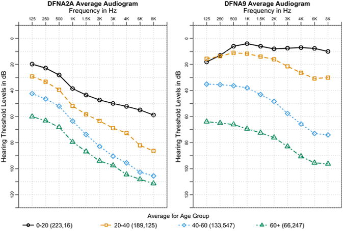
Sample audioprofiles from the averages of patients from DFNA2A and DFNA9 grouped into age groups spanning two decades. Average standard deviation across all ages and frequencies is 18.92 dB and 19.47 dB for DFNA2A and DFNA9, respectively. This same plot with error bars is shown in Supp. Figure 1. The number of audiograms for each age group is listed in parentheses in the legend, with the number of audiograms for DFNA2A listed first and then DFNA9. Both loci exhibit distinctly different shapes of hearing loss along with different rates of progression over time.

In this article, we describe the algorithms, procedures, and methods used to conduct automatic prioritization of genetic loci based on patient-derived audiograms. This prioritization procedure results in a ranked list of genetic loci for a given audioprofile. These methods are used both in a large-scale pipeline to classify sets of audiograms submitted for analysis, as well as a web-based portal for independent analysis of audiograms from patients or their physicians. In most cases, the steps outlined apply to both training data as well as previously unclassified audiograms.

Methods

Audiometric Data

The dataset used to train AudioGene consists of audiograms collected from publications, original audiograms provided by authors, and by otolaryngology and audiology clinics. Our dataset was comprised of 3,312 audiograms from 1,445 patients. The typical audiogram included data for six frequencies: 250Hz, 500Hz, 1kHz, 2kHz, 4kHz, and 8kHz. Audiograms based on fewer than four frequency points were excluded. To date, we have developed four versions of AudioGene based on the number of available audiograms – in the latest version, after processing 3,024 audiograms are included in the training set. The total number of patients and audiograms for each locus is listed in Supp. Table S1.

Preprocessing

Audiograms in the dataset were preprocessed prior to their use in prioritization or training. If available, audiograms from both ears taken at the same time were combined by retaining the minimum value (i.e. better acuity) at each frequency. This results in a composite audiogram that has the least amount of hearing loss at each frequency. Coefficients of second and third order polynomials were then fit to each audiogram and added as secondary features. Linear interpolation and extrapolation were used next to replace missing threshold values. Each collection of patient-derived audiograms was grouped into a ‘bag’ for use with multi-instance classifiers, with a one-to-many relationship between patients and audiograms (Auer, 1997). For classifiers that did not support multi-instance datasets, each bag was reduced to a single representative audiogram using the geometric average of the audiograms in the bag.

Prioritization

Patient audiograms collected during clinical care visits as part of a diagnostic protocol (referred to subsequently as ‘unknown’ audiograms) were ranked according to the probabilities generated by a modified Support Vector Machine (SVM) using a linear kernel capable of utilizing multi-instance datasets, which was already implemented in Weka (Frank et al., 2004; Hall et al., 2009). SVM training was performed using the Sequential Minimization Optimization algorithm (SMO), in which a one-versus-one strategy is used to handle multiple classes in conjunction with pair-wise coupling to generate the probabilities for each locus (Vapnik, 1995; Platt, 1998). Since probabilities of SVMs are not well calibrated, they are only useful in ranking. The multi-instance SVM processes the bagged audiograms at the kernel level, where the kernel distance between two patients is the sum of all pairwise kernel distances between all pairs of audiograms in each patient's bag. The loci/genes are then ranked in decreasing order of probability to produce a prioritized list of loci to inform genetic testing efforts. While these probabilities are useful for ranking they are not regularized, and are therefore only useful as relative probabilities.

Classifier Choice

Five different classifiers were evaluated using two strategies. 1) Accuracy, area under ROC curves (AUC), precision and recall were computed for each classifier using ten 10-fold cross-validation experiments. AUC, precision and recall were then computed for each class using a weighted average based on the size of each locus. 2) We performed a leave-one-out analysis of the aforementioned prioritization method using each classifier. Audiogram bags corresponding to each patient were removed from the training set one at a time, and the prioritization method was performed with the classifier being evaluated. For this analysis, patients were considered correctly classified if their locus was ranked amongst the top N loci, using the ranking method described in the previous section. SVM, Multi-instance SVM, a Majority classifier, Random Forest (Breiman, 2001), and Bagging (Breiman, 1996) were each tested as classifiers. Both SVM implementations used a linear kernel and all of the classifiers were derived from implementations in Weka (Hall et al., 2009). The Majority classifier was considered the baseline against which the performance of all others was measured.

Validating Preprocessing

A leave-one-out analysis of various combinations of preprocessing steps was performed on the training set. These permutations included combining only audiograms taken from different ears at the same age, combining and filling in missing (frequency) values, and adding the coefficients of fitted second- and third-order polynomials.

Noise Model and Robustness to Noise

A noise model was developed by representing real-world noise associated with the measurement and recording of audiometric data (Figure 2). This model was then used to perform a simulation to determine the robustness of our method in the presence of noise. The noise model takes into consideration a mis-calibrated audiometer and test-retest variability (Schmuziger et al., 2004). According to our model, a mis-calibrated audiometer could result in an additive (+/−) shift across an entire audiogram, and the test-retest variability may introduce up to a 10 dB difference between measurements taken at two different times for the same patient. The noise model adds noise in the frequency domain. In other words, the added noise is based on treating the frequency values as values in the domain (x-axis) and the dB loss/gain as values along the range (y-axis). The Discrete Cosine Transform (DCT) (Ahmed and Natarajan, 1974) was used to transform the audiogram curves into the frequency domain. The DCT was chosen over the Fourier transform for simplicity, because all DCT components are all real-valued. The DCT transform function F is shown in Equation 1.

Figure 2. Audiogram with noise added.

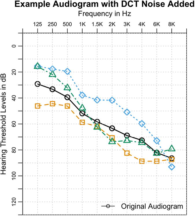
An audiogram with three examples of added noise, with a ShiftScale of 10 and Scale of 5. The overall characteristic shape of the audiogram still remains after noise is applied.

$$F_k=a_k\sum _{n=0}^{N-1}{f}_n\text{cos}(\frac{\pi }{N}(n+\frac{1}{2})k),k=0,\dots ,N-1$$

$$\text{where}{a}_k=\{\begin{array}{c}\frac{1}{\sqrt{N}}k=0\\ \sqrt{\frac{2}{N}}k>0\end{array}$$

Once in the frequency domain, noise is added in two parts. First, a random magnitude of noise is added to F₀ (the DC component) in order to shift the entire audiogram. This mimics the case where the calibration of the audiometer results in uniform inaccuracy for the entire measurement of the audiogram. Next, Gaussian noise is added to the other coefficients with a magnitude scaled by an exponential decay function. This simulates the test-retest variability discussed above. The exponential decay function effectively concentrates the noise in lower frequency components of the DCT and results in noisy audiograms that still retain their overall characteristic shape. With the addition of this noise, an inverse DCT was performed to recreate a time-domain audiogram. A few examples of the noise added to an audiogram are shown in Figure 2, with ShiftScale at 10 and Scale at 5. We define ShiftScale as a scalar value that controls the magnitude with which the audiogram can be shifted, and Scale as a variable used to control the degree with which overall curve shape is changed. Lower values of both of these variables mean lower noise, and vice versa. To determine the robustness of our prioritization method to noise, 5% of the patients were selected at random and removed from the training set.

Noise was added to the removed audiograms using our noise model, with the value of ShiftScale always twice as large as the value of Scale. For a given level of noise x, ShiftScale and Scale are typically 5x and 2.5x, respectively. The prioritization method was then trained on the remaining 95% of patients, and the 5% withheld subset was classified. This process was repeated 200 times with a different random sampling of patients on each repetition. The final accuracy for a given ranking requirement (N) is the sum of all the patients that were correct across all iterations divided by the total number of patients that were withheld over all 200 iterations. The value of N specifies that the locus/gene must be ranked amongst the top N loci/genes given by the prioritization method described in the Prioritization section.

Identifying Outliers

A variant of the leave-one-out analysis was used to identify patients who are outliers to the classifier and are often misclassified. Each patient was removed and the classifier was retrained on the remaining patients. The noise model described in the previous section was used to add noise to the removed patient's audiograms, with a noise Scale of 5. The patient was then classified with the retrained classifier, and the predicted locus was recorded. The classification was repeated 100 times with the noise model applied each time to the patient's original audiograms. If the correct locus was never predicted for any of the 100 iterations, the patient was considered an outlier.

Web Interface

AudioGene is accessible via a web interface (http://audiogene.eng.uiowa.edu) and all analyses are performed on secure servers managed by the Center for Bioinformatics and Computational Biology (CBCB) at the University of Iowa. Audiometric data may be uploaded via a web-based spreadsheet form or by using a downloadable Excel™ spreadsheet provided on the website. After uploading data, audiograms are displayed as images to validate data entry. Once verified, the analysis can be completed using all available loci or a user-selected subset of these loci, an option that can be chosen when specific loci have already been excluded. Uploaded and verified data are submitted to a local computational cluster in the CBCB for analysis. When predictions are complete, results are made available to users online and by e-mail. Successful application of this website to genetic hearing loss has been demonstrated by the authors and others (de Heer et al., 2011).

Results

Comparison of Classifiers and Performance

Bagging, Random Forest (RF), and Multi-Instance SVM (MI-SVM) had very comparable performance (Table 1), and ROC curves for each class for these classifiers are shown in Supp. Figure S2. However, their performance differs when measuring accuracy over various values of N. At higher values of N, when plotting accuracy versus the number of guesses, MI-SVM and Single-Instance SVM (SI-SVM) outperform all other classifiers (Figure 3). The MI-SVM and SI-SVM have approximately equal accuracies at higher values of N but for lower values, the MI-SVM performs better. Both the Random Forest classifier (RF) and Bagging classifier perform as well as the MI and SI-SVMs at lower values of N, but at higher values of N, their accuracy reaches a maximum of approximately 91%, whereas the MI- and SI-SVMs approach 100%. This difference is due to limitations in the training methods, since loci for which there are only a few audiograms are never predicted. Based on this analysis, we chose to use the MI-SVM as the classifier for AudioGene. It has an estimated accuracy of 68% of including the correct locus/gene in the top 3 predictions. In contrast, the Majority classifier has an accuracy of only 47%. This measurement of performance is a good metric because it is similar to the intended use of AudioGene, where clinicians would sequence the predicted genes in an iterative fashion, often-times quite rapidly (days). This approach allows us to determine our accuracy in the event that multiple predictions are required before identifying the correct locus.

Table 1. Classifier Performance.

Accuracy, AUC, precision and recall for all classifiers tested. Bold values indicated the highest value, and multiple bold values indicate that they were statistically the same. AUC, precision, and recall were all computed as weighted averages based on the size of each locus.

Classifier	Accuracy	AUC	Precision	Recall
Bagging	43.86% (3.06)	0.82 (0.02)	0.37 (0.03)	0.44 (0.03)
RF	43.14% (3.16)	0.71 (0.16)	0.37 (0.04)	0.43 (0.03)
MI-SVM	42.95% (2.91)	0.80 (0.16)	0.31 (0.03)	0.43 (0.03)
SVM	40.99% (2.57)	0.79 (0.17)	0.26 (0.02)	0.41 0.03
Majority	19.72% (0.34)	0.50 (0.00)	0.04 (0.00)	0.20 0.00

Figure 3. Classifier Performance over various N.

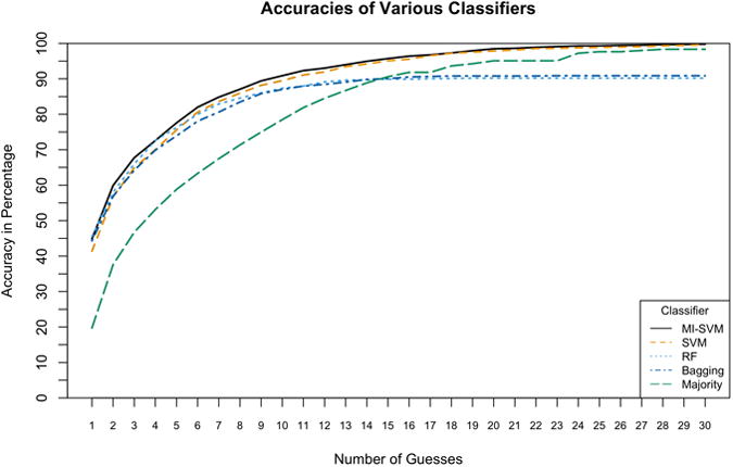
A comparative plot of the accuracy of the evaluated classifiers. This plots accuracy against N, where N represents whether or not the correct locus was ranked among the top N loci. Both SVMs outperform all other classifiers and the Multi-Instance SVM (MI-SVM) demonstrates the best accuracy of all.

Preprocessing Validation

Raw data without any preprocessing outperform any of the other preprocessing steps at higher values of N. We hypothesized that this was due to a bias in which frequency measurements are not randomly missing, but rather are dependent upon their constitutive loci (Figure 4). This hypothesis was evaluated by converting audiograms into binary vectors in which each frequency value was coded as 1 if a threshold measurement is available or 0 if there is no measurement. A10-fold cross-validation was then run with an SVM and its accuracy was compared against a Majority classifier. Accuracies should be similar if no information is contained in the missing frequency values, but the MI-SVM produced an accuracy of 33% while the Majority classifier had an accuracy of 20%. Therefore, filling the missing values must be done to eliminate this bias.

Figure 4. Preprocessing Validation.

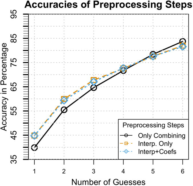
The accuracies of different combinations of preprocessing steps. While preprocessing with only combining audiograms taken at the same age but from different ears has greater accuracy as the number of guesses increase, it has been shown that this is due to a collection bias. Interpolating missing values is therefore necessary in order to remove this bias. Even though adding the coefficients of fitted second and third order polynomials produces marginal increase in performance, it has been shown in a follow-up experiment to be statistically significant.

On the basis of this analysis, we did not include a comparison of the effect of adding only the polynomial coefficients. As Figure 4 shows, adding the coefficients has only a marginal effect on the accuracy. To prove statistical significance, 10-fold cross-validation experiments were performed as a follow-up to compare the addition of the coefficients. The accuracy of identifying the correct gene/locus within the first three predictions was 66.05% with the coefficient added, versus 65.22% without. This small gain improves performance and is computationally inexpensive to compute. We therefore included a preprocessing step that consists of adding the coefficients of fitted second and third order polynomials and filling in missing values.

Robustness to Noise

AudioGene suffers minor performance degradation from its baseline performance over modest amounts of noise (∼3% at noise levels between 1 and 3, as defined previously), as shown in Figure 5. It is only with higher levels of noise that there is a significant loss of performance (∼10%). This amount of noise would equate to a shift of the audiogram between 20 and 25 dB and substantial distortion to the original audiogram's shape.

Figure 5. Noise Analysis.

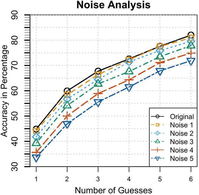
The result of the noise analysis with varying degrees of noise versus performance of the ‘top N loci’ selection method compared to the classification performance with no noise (the original). From this plot, it is shown that AudioGene is robust to the amount of noise expected from mis-calibration and test-retest variability.

Outlier Identification

A patient's audiogram was considered an outlier if the correct gene/locus was never predicted during any of 100 repetitions with the addition of high amounts of noise. The plot of outliers by loci is shown in Supp. Figure S3. We can infer that, to the classifier, patients who are outliers never appear similar to other patients from that locus.

As a general rule, smaller loci (in terms of the number of patients per locus) should contain a larger percentage of outlier patients and conversely, larger loci should contain fewer outliers. However, there exist some loci that have a larger number of outliers than expected. DFNA10 is an example in which 34 of 56 patients are labeled as outliers. Further investigation of these outliers is necessary to determine if they are truly outliers or are representative of the inherent variability of the audiograms for a particular locus.

Discussion

In this paper, we present a method for predicting genotypes based on phenotypes in patients segregating ADNHSL, and our complete pipeline can be seen in Figure 6. We show that the most robust performance was achieved using MI-SVM, and that this approach has an accuracy of ∼68% as compared to a Majority classifier, which has an accuracy of ∼44%. Missing threshold values must be interpolated to guarantee an unbiased classifier that generalizes effectively to unknown data.

Figure 6. Final Pipeline.

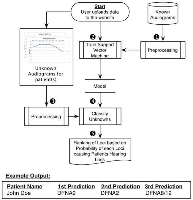
The final analysis pipeline of AudioGene used to make predictions for unknown patients. (1) The training set is preprocessed by filling in missing values and adding coefficients of fitted second and third order curves. (2) A Multi-Instance SVM is trained on the preprocessed training set from step 1. (3) Unknown patients' audiograms are preprocessed in the same manner as described in Step 1. (4) Probabilities for each locus are generated by the trained SVM model. (5) Loci are finally ranked by their probabilities, with results being displayed on the website and emailed to the user.

In some settings, missing data can serve as informative features. For example, a missing value from a “date of death” field implies that the patient is not deceased. In the case of an audiogram, missing frequency thresholds imply nothing about the phenotype of the patient, but rather are normal variations in clinical practice between sites. Therefore, missing thresholds must be interpolated to guarantee an unbiased classifier, otherwise the classifier cannot generalize effectively to data collected at different clinics.

Our data show that AudioGene is robust to modest levels of noise. Although we attempted to employ a simple linear model to apply random amounts of noise independently at each frequency, this approach generated physically impossible audiograms and was abandoned. An example is a saw tooth-patterned audiogram produced by alternating +/−10 dB at each frequency. By applying noise in the frequency domain with the DCT, we retained the overall audioprofile but produced audiograms that were shifted and/or stretched but still physically possible. This model allowed us to tune the noise so that we could test the addition of varying amounts of noise and also enabled us to identify outliers.

The identification of outliers is particularly interesting, since genetic modifiers of hearing loss are known to exist. Our method for identifying outliers is equivalent to selecting the patients who are not predicted correctly, even when allowing for large degrees of error in the data collection. This could be caused by inadequate training data for a given locus, inadequate separation between two phenotypically similar loci, an improperly assigned causative locus, or environmental and genetic modifiers that affect the patient's phenotype.

In summary, we have developed a method for prioritizing genetic loci for ADNSHL screening based on a patient's phenotype. Using a leave-one-out analysis, AudioGene has an estimated accuracy of 68% for identifying the correct genetic cause of hearing loss within the top three predictions using a MI-SVM. The method is robust to noise with a drop in accuracy only when large amounts of noise are applied. AudioGene is available as a web service at http://audiogene.eng.uiowa.edu. Originally developed for prioritizing loci for Sanger sequencing (Hildebrand et al., 2008; Hildebrand et al., 2009), as technologies have advanced, AudioGene has proven invaluable as a method of evaluating variants of unknown significance generated by targeted genomic capture and massively parallel sequencing, effectively linking a person's phenome to their genome (Shearer et al., 2010; Eppsteiner et al., 2012).

References

- Ahmed N, Natarajan T. Discrete Cosine Transform. IEEE Trans Computers. 1974:90–93. [Google Scholar]
- Auer P. On Learning From Multi-Instance Examples: Empirical Evaluation of a Theoretical Approach; Proceedings of the Fourteenth International Conference on Machine Learning; 1997. pp. 21–29. [Google Scholar]
- Breiman L. Bagging predictors. Machine Learning. 1996;24:123–140. [Google Scholar]
- Breiman L. Random Forest. Machine Learning. 2001;45:5–32. [Google Scholar]
- de Heer AMR, Schraders M, Oostrik J, Hoefsloot L, Huygen PLM, Cremers CWRJ. Audioprofile-directed successful mutation analysis in a DFNA2/KCNQ4 (p.Leu274His) family. Ann Otol Rhinol Laryngol. 2011;120:243–248. doi: 10.1177/000348941112000405. [DOI] [PubMed] [Google Scholar]
- Eppsteiner RW, Shearer AE, Hildebrand MS, Taylor KR, Deluca AP, Scherer S, Huygen P, Scheetz TE, Braun TA, Casavant TL, Smith RJH. Using the Phenome and Genome to Improve Genetic Diagnosis for Deafness. Otolaryngol Head Neck Surg. 2012 doi: 10.1177/0194599812454271. [DOI] [PMC free article] [PubMed] [Google Scholar]
- Frank E, Hall M, Trigg L, Holmes G, Witten IH. Data mining in bioinformatics using Weka. Bioinformatics. 2004;20:2479–2481. doi: 10.1093/bioinformatics/bth261. [DOI] [PubMed] [Google Scholar]
- Hall M, Frank E, Holmes G, Pfahringer B, Reutemann P, Witten IH. The WEKA data mining software. SIGKDD Explor Newsl. 2009;11:10–18. [Google Scholar]
- Hildebrand MS, Deluca AP, Taylor KR, Hoskinson DP, Hur IA, Tack D, McMordie SJ, Huygen PLM, Casavant TL, Smith RJH. A contemporary review of AudioGene audioprofiling: a machine-based candidate gene prediction tool for autosomal dominant nonsyndromic hearing loss. Laryngoscope. 2009;119:2211–2215. doi: 10.1002/lary.20664. [DOI] [PMC free article] [PubMed] [Google Scholar]
- Hildebrand MS, Morín M, Meyer NC, Mayo F, Modamio-Hoybjor S, Mencía A, Olavarrieta L, Morales-Angulo C, Nishimura CJ, Workman H, Deluca AP, Del Castillo I, et al. DFNA8/12 caused by TECTA mutations is the most identified subtype of non-syndromic autosomal dominant hearing loss. Hum Mutat. 2011 doi: 10.1002/humu.21512. [DOI] [PMC free article] [PubMed] [Google Scholar]
- Hildebrand MS, Tack D, McMordie SJ, DeLuca A, Hur IA, Nishimura C, Huygen P, Casavant TL, Smith RJH. Audioprofile-directed screening identifies novel mutations in KCNQ4 causing hearing loss at the DFNA2 locus. Genetics in Medicine. 2008;10:797–804. doi: 10.1097/GIM.0b013e318187e106. [DOI] [PMC free article] [PubMed] [Google Scholar]
- Hilgert N, Smith RJH, Van Camp G. Forty-six genes causing nonsyndromic hearing impairment: which ones should be analyzed in DNA diagnostics? Mutat Res. 2009;681:189–196. doi: 10.1016/j.mrrev.2008.08.002. [DOI] [PMC free article] [PubMed] [Google Scholar]
- Leonard D, Shen T, Howe H, Egler T. Trends in the prevalence of birth defects in Illinois and Chicago 1989 to 1997. Springfield, IL: Illinois Department of Public Health; 1999. [Google Scholar]
- Mohr PE, Feldman JJ, Dunbar JL, McConkey-Robbins A, Niparko JK, Rittenhouse RK, Skinner MW. The societal costs of severe to profound hearing loss in the United States. Int J Technol Assess Health Care. 2000;16:1120–1135. doi: 10.1017/s0266462300103162. [DOI] [PubMed] [Google Scholar]
- Platt JC. Sequential minimal optimization: A fast algorithm for training support vector machines. Advances in Kernel MethodsSupport Vector Learning. 1998;208:1–21. [Google Scholar]
- Schmuziger N, Probst R, Smurzynski J. Test-retest reliability of pure-tone thresholds from 0.5 to 16 kHz using Sennheiser HDA 200 and Etymotic Research ER-2 earphones. Ear Hear. 2004;25:127–132. doi: 10.1097/01.aud.0000120361.87401.c8. [DOI] [PubMed] [Google Scholar]
- Shearer AE, Deluca AP, Hildebrand MS, Taylor KR, Gurrola J, Scherer S, Scheetz TE, Smith RJH. Comprehensive genetic testing for hereditary hearing loss using massively parallel sequencing. Proc Natl Acad Sci USA. 2010;107:21104–21109. doi: 10.1073/pnas.1012989107. [DOI] [PMC free article] [PubMed] [Google Scholar]
- Shearer AE, Hildebrand MS, Sloan CM, Smith RJH. Deafness in the genomics era. Hear Res. 2011;282:1–9. doi: 10.1016/j.heares.2011.10.001. [DOI] [PMC free article] [PubMed] [Google Scholar]
- Smith RJ, Bale JF, Jr, White KR. Sensorineural hearing loss in children. The Lancet. 2005;365:879–890. doi: 10.1016/S0140-6736(05)71047-3. [DOI] [PubMed] [Google Scholar]
- Snoeckx RL, Huygen PLM, Feldmann D, Marlin S, Denoyelle F, Waligora J, Mueller-Malesinska M, Pollak A, Ploski R, Murgia A, Orzan E, Castorina P, et al. GJB2 mutations and degree of hearing loss: a multicenter study. Am J Hum Genet. 2005;77:945–957. doi: 10.1086/497996. [DOI] [PMC free article] [PubMed] [Google Scholar]
- Stierman L. Birth defects in California: 1983–1990. California Department of Health Services; 1994. [Google Scholar]
- Thompson DC, McPhillips H, Davis RL, Lieu TL, Homer CJ, Helfand M. Universal newborn hearing screening: summary of evidence. JAMA. 2001;286:2000–2010. doi: 10.1001/jama.286.16.2000. [DOI] [PubMed] [Google Scholar]
- Van Camp G, Smith RJH. The Hereditary Hearing loss Homepage. 2012 Available from: http://hereditaryhearingloss.org/
- Vapnik V. The nature of statistical learning. Springer; 1995. [Google Scholar]
- White KR. The current status of EHDI programs in the United States. Ment Retard Dev Disabil Res Rev. 2003;9:79–88. doi: 10.1002/mrdd.10063. [DOI] [PubMed] [Google Scholar]
- White KR. Early hearing detection and intervention programs: opportunities for genetic services. Am J Med Genet A. 2004;130A:29–36. doi: 10.1002/ajmg.a.30048. [DOI] [PubMed] [Google Scholar]
Associated Data
This section collects any data citations, data availability statements, or supplementary materials included in this article.