Detection of epileptic activity in fMRI without recording the EEG

Abstract

EEG–fMRI localizes epileptic foci by detecting cerebral hemodynamic changes that are correlated to epileptic events visible in EEG. However, scalp EEG is insensitive to activity restricted to deep structures and recording the EEG in the scanner is complex and results in major artifacts that are difficult to remove.

This study presents a new framework for identifying the BOLD manifestations of epileptic discharges without having to record the EEG. The first stage is based on the detection of epileptic events for each voxel by sparse representation in the wavelet domain. The second stage is to gather voxels according to proximity in time and space of detected activities.

This technique was evaluated on data generated by superposing artificial responses at different locations and responses amplitude in the brain for 6 control subject runs. The method was able to detect effectively and consistently for responses amplitude of at least 1% above baseline. 46 runs from 15 patients with focal epilepsy were investigated. The results demonstrate that the method detected at least one concordant event in 37/41 runs. The maps of activation obtained from our method were more similar to those obtained by EEG–fMRI than to those obtained by the other method used in this context, 2D-Temporal Cluster Analysis. For 5 runs without event read on scalp EEG, 3 runs showed an activation concordant with the patient’s diagnostic.

It may therefore be possible, at least when spikes are infrequent, to detect their BOLD manifestations without having to record the EEG.

Introduction

Functional MRI (fMRI) is now established as a powerful tool for the presurgical evaluation of refractory epilepsy. fMRI can predict the possible deficits in visual, language, motor or sensory functions that would arise from a surgical intervention. fMRI can also be used to help in the evaluation of epileptic foci. The difficulty of this technique is to identify the timing of epileptic activity. Simultaneously acquired electroencephalogram (EEG) and fMRI allows the timing of the events seen on EEG to be locked to the blood oxygen level dependent (BOLD) signal, allowing the examination of hemodynamic changes in the brain that correlate to epileptic events. EEG–fMRI is a technique that combines the high temporal resolution of scalp EEG with the high spatial resolution of BOLD signal. Many studies showed the usefulness of EEG–fMRI to characterize various forms of focal and generalized epilepsy (Aghakhani et al., 2004; Kobayashi et al., 2006; Salek-Haddadi et al., 2006; Tyvaert et al., 2008; Zijlmans et al., 2007). Unfortunately, scalp EEG is insensitive to activity restricted to deep structures or discharges with an unfavorable dipole orientation for scalp recordings. Moreover, recording the EEG in the scanner is complex and results in major artifacts that are difficult to remove (ballistocardiogram–gradient artifact). Finally this technique is useful only in patients with frequent interictal events recorded from the scalp EEG. The challenge of this study is to propose a method for identifying the BOLD manifestations related to epileptic events without having to record the EEG.

Common fMRI analyses use a convolution between the paradigm and the hemodynamic response function (HRF). A related problem is that the nature, timing and duration of the events (paradigm) are hard to specify a priori. An alternative analysis strategy that may be appropriate in such situations is the data-driven approach. Data-driven approaches ignore the underlying physiology and attempt to determine the intrinsic structure of the data. These methods are applied to obtain a simplified data representation of the raw data that performs data reduction. The most popular methods are principal component analysis (PCA) for which the derived components are orthogonal to each other (Baumgartner et al., 2000); and independent component analysis (ICA) for which the sources (signal and noise) are statistically independent (Beckmann and Smith, 2004). Other data-driven techniques such as clustering (Fadili et al., 2000) and temporal clustering analysis (TCA) (Morgan et al., 2004) can be used. Although ICA-based approaches may be able to accurately estimate the number of components using cross-validation (Varoquaux et al., 2010), most of them need manual intervention to estimate a priori the number of components or clusters, and then to distinguish the noise-related from neurophysiologic-relevant components or clusters.

TCA is the only method that has been used in the detection of BOLD responses to epileptic events of unknown timing. This technique gathers voxels based on the timing of their first activation and may be efficient due to the high temporal synchronicity associated with epileptic activity. A modified version of TCA, called 2D-TCA, has shown some success for the detection of fMRI activity in epilepsy (Morgan et al., 2007). We recently showed, however, that 2D-TCA could only detect epileptic activity if enough events were recorded during an fMRI run and if the HRF associated with those events was of sufficient amplitude (Khatamian et al., 2011). Moreover, the method often provided components describing other activity not associated with epilepsy but it does not separate them.

Another class of methods for fMRI data analysis is called model-based approaches. Model-based approaches assume a more or less complete mathematical model of the data. The General Linear Model is the most common method. It assumes that the shape of the HRF is known. An accurate estimate of the HRF is crucial to prevent false positive and negative results (Lindquist and Wager, 2007). While a Glover HRF (Glover, 1999) is commonly used for fMRI analyses, studies have shown a significant variability of the HRF for different types of epileptiform discharges across subjects (Benar et al., 2002). To overcome these problems, parameterized HRF approach can be used (Makni et al., 2008; Woolrich et al., 2004). The benefit of the parameterization is to separately represent different shape characteristics of the HRF.

Our approach is similar to the so-called “blind deconvolution”. Most of the methods in Bayesian formulation used the prior hypothesis that the timings of events are a Bernoulli process (Champagnat et al., 1996). The first step is the detection of the timings and is followed by the magnitude estimation. In this study, we detected the timings of events by using a dictionary of HRF in the wavelet domain. Recently, Khalidov et al. (2011) introduced a new dictionary, called “activelets”. These wavelets have the benefit to approximate well a class of gamma-functions HRF models based on the balloon model, instead of having a single HRF model. Moreover, these wavelets compact the activation energy on a few coefficients, so in the case of sparse paradigm, the response will also be sparse and this is why a sparse representation is useful to select the most significant wavelet coefficients. The study of Khalidov et al. showed that these new wavelets were well suited for the activation-related signal in fMRI without knowledge of the actual onset times. However, they only showed the ability of this dictionary to detect activation associated with visual stimulation in a small region-of-interest.

The aim of our study was to propose a new framework for identifying the timing of epileptic events in fMRI BOLD signals without recording the EEG. Our method is based on an activelets dictionary and a sparse representation to detect epileptic activities in each voxel and then a spatio-temporal clustering to gather voxels according to timing of detected activity and spatial information. Validations of such methods can be difficult due to the absence of a “gold standard” with which to corroborate the results. Consequently, we first validated the method using simulated data obtained from healthy subjects and then we showed the effectiveness of the method for 15 epileptic patients compared to EEG–fMRI.

Methods

Data acquisition

Data were selected from a database of focal epilepsy patients and control subjects who underwent EEG–fMRI. Functional images were continuously acquired using a 3 T Siemens Trio Scanner. The functional data were acquired over 6 min runs using ${\text{T}}_2^{\ast }$-weighted EPI sequence (TR=1.75 s, TE=30 ms, flip angle of 90°, 5 mm isotropic voxel size, 64×64 matrix, 25 transverse slices). A T₁-weighted anatomic acquisition (TR=23 ms, TE=7.4 ms, flip angle of 30°, 1 mm isotropic voxel size, 256×256 matrix, 176 sagittal slices) was used for superposition with the functional images and for defining a brain mask.

Multiple 6-min runs were performed up to 2 h, unless patients experienced discomfort or if they suffered from clinical events susceptible of causing injuries. During the fMRI scanning, simultaneous EEG was recorded using 25 MR-compatible Ag/AgCl electrodes positioned on the scalp according to the 10–20 system (19 standard locations), with additional electrodes at F9-T9-P9 and F10-T10-P10, and referenced to FCz. Two additional electrodes on the back recorded the electrocardiogram. The EEG was low pass filtered at 1 kHz and sampled at 5 kHz with a BrainAmp amplifier (Brain Products, Gilching, Germany). After scanning, correction of gradient artifacts was performed using an averaged subtraction method (Allen et al., 2000) implemented in BrainVision Analyzer software (Products, Gilching, Germany). The ballistocardiogram artifact was then removed by an ICA method (Benar et al., 2003). Finally, a neurologist reviewed the EEG and marked the timing of epileptic activity.

Simulated data

Simulated data were used according to previous studies (Khatamian et al., 2011; LeVan and Gotman, 2009). Artificial time courses were created by simulating epileptic activity at different locations in the brain for 6 control subject runs. The EEGs of these runs were checked to ensure that no abnormal activity was present. Simulated responses were created by generating epileptic-like activity at random timings and convolving them with a HRF function (a Glover HRF (Glover, 1999) or its temporal derivative or a gamma function). The choice of the HRF was random. Three volumes of interest (VOIs) (right frontal lobe, left temporal lobe, and right hippocampus) were selected to simulate activity related to spikes by using all combinations of the following parameters: 1, 5, or 10 randomly generated spike timings per 6-min run (sufficiently sparse in time to avoid nonlinearities, see below); HRF amplitudes between 0.5% and 2%, above the mean fMRI signal value, in 0.25% increments; and VOIs of 12, 27, 36, 64, 80, and 125 voxels. An additional dataset was created using a single randomly timed 5 s long event in a parietal lobe VOI with the above HRF amplitudes in VOIs of 64, 125, and 216 voxels, to represent a short seizure.

In summary, each simulated run contained 4 VOIs with 4 forms of epileptic activity (i.e. 1 spike, 5 spikes, 10 spikes, and one 5 s event). There were 6 control subject scans, 6 VOI sizes, 7 HRF amplitudes, yielding 252 simulated datasets.

Proposed method

For the purpose of detecting epileptic activity in fMRI without information on when the activation occurs or on the shape of the HRF, it was critical to make some assumptions. We first assumed that the hemodynamic responses were sufficiently sparse in time to have a linear response. Although, they are not very large, non-linearities have been noted when events are close in time (Bagshaw et al., 2005). Secondly, we assumed a spatial coherence in the mapping of the activation. Several voxels inside the same region must have the same kind of temporal events. The proposed method is a two-stage approach. The first identifies the timings of epileptic events for each time course (voxel) based on the sparsity of events and the second stage gathers voxels with similar event timings and similar spatial distribution. A weight was added to the clustering stage in order to give more importance at voxels with similar event timings than voxels with similar spatial distribution. All fMRI data were pre-processed by applying slice time correction, motion correction, and spatial smoothing (6 mm FWHM). A brain mask, defined from the anatomical MRI, was created to remove voxels outside of the brain.

Detecting the timing of epileptic activity for each time course

In this stage, the hemodynamic system is assumed to be linear and shift-invariant, which are common assumptions in fMRI analyses. Thus, we can model each BOLD signal as follows:

$$\text{y}[\text{t}]=\sum _{\text{k}}{\text{A}}_{\text{k}}\text{h}[\text{t}-{\text{t}}_{\text{k}}]+\text{n}[\text{t}].$$ (1)

Where A_k and t_k are the activity amplitude and activity onset, respectively. These parameters were unknown in our study and we used a dictionary of functions for modeling the hemodynamic system h. The parameter n of Eq. (1) corresponds to the noise term including baseline, trend, and noise. It was removed by applying a normalization step (the time series were corrected to zero mean and unit variance), then the voxel time courses were detrended by removing a fitted polynomial regression model from the time courses (Worsley et al., 2002), and finally an autoregressive model (order 1) was applied. Although the noise structure is correlated in space (Worsley et al., 2002), we considered the fMRI BOLD signal independent in space. We neglected the spatial dependencies of noise because we think that our model itself is flexible enough to account for HRF shape fluctuations. Eq. (1) became:

$$\text{y}[\text{t}]=\sum _{\text{k}}{\text{A}}_{\text{k}}\text{h}[\text{t}-{\text{t}}_{\text{k}}]+\mathrm{\epsilon }[\text{t}].$$ (2)

Where ε_t is a white random vector. The main issue was then to identify the timing of BOLD activity. Studies using a threshold value to detect the activities have shown low specificity because of the weak BOLD contrast that exists in the hemodynamic response (Khatamian et al., 2011). We propose to use a more robust thresholding technique. Wavelet analysis has led to many successful signal and image processing algorithms, including thresholding techniques (Crouse et al., 1998; Donoho and Johnstone, 1994). The ability of wavelet transform to pack the most signal energy in few large coefficients is behind the success of wavelet-based thresholding algorithms. Although the wavelet transform has been applied to fMRI time course processing, the traditional wavelets are not well-suited for the detection of activity in BOLD signal because no information about the shape of the HRF is introduced. Two popular frameworks for the hemodynamic model are the “balloon model” (Buxton et al., 1998) and the “windkessel model” (Mandeville et al., 1999). Recently, Khalidov et al. (2011) showed a new wavelet basis, called “activelets”, which is able to model the hemodynamic system by using a linear approximation of the expanded balloon model (Friston et al., 2000) for the HRF. These wavelets depend on one vector α⃗ and one scalar γ, which are expressed in terms of hemodynamic parameters of this model (Khalidov, 2009) (see Appendix A). The definition of activelets is also explained in this appendix.

Different shapes of the wavelet function can be obtained by changing the hemodynamic parameters (Fig. 1). We have optimized these two degrees of freedom by minimizing the reconstruction error of several HRFs (Glover function, gamma function and its derivative). An activelet decomposition was applied to each HRF by using an undecimated wavelet transform with 3 scales in the decomposition. Five wavelet coefficients were sufficient to reconstruct different shapes of HRF (canonical and gamma functions) with an average SNR of 30 dB. In comparison, to obtain the same quality using regular wavelets (Haar–Daubechies — B-spline), 30 coefficients are needed. Fig. 2 illustrates the activelet basis in a multiscale decomposition. The dilated versions of the scaling and wavelet functions show the ability for capturing different shapes of HRF.

Fig. 1.

The effects of changing the balloon parameters on the activelet basis. (top) Scaling functions and (bottom) wavelet functions in varying the parameter α in the balloon model. In this case, the time to peak is different following the value of α.

Fig. 2.

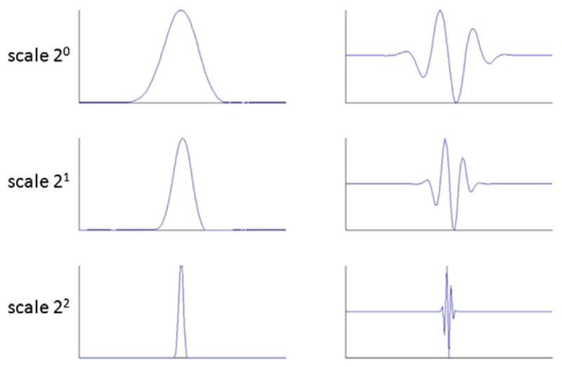
Multiscale representations of scaling function (left) and wavelet functions (right) of the activelet basis.

Activelets form a dictionary of basis functions in which the hemo-dynamic response is sparsely represented and these wavelets model the hemodynamic system by using a linear approximation of the balloon model for the HRF (common assumption in fMRI analyses). This linearity assumption assumes that the events must be sufficiently sparse in time, as discussed above. This is why a sparse representation algorithm was used to select the activelet coefficients giving the sparsest solution β₀ for each voxel, i.e. the solution with the smallest possible number of epileptic events. This is achieved by imposing a l1-norm penalty in the transform domain:

$${\mathrm{\beta }}_0=arg\underset{\mathrm{\beta }}{min}\left(\frac{1}{2}{\Vert \text{y}-\mathrm{\Phi }\mathrm{\beta }\Vert }_2^2+\lambda {\Vert \mathrm{\beta }\Vert }_1\right).$$ (3)

Where Φβ is the reconstruction of a signal on the activelets basis Φ (Φ^T is the undecimated wavelet transform obtained by performing the “a trous” algorithm). Each activelet filter is normalized with respect to its l₂ norm; β is the solution vector and λ is the regularization parameter. All degrees of freedom were empirically set for the best performance on simulated data. Although we kept the values giving the best performance, each parameter had a stability range. λ was set to 0.5. This parameter controls the sparsity of the solution. The solution is sparser when λ is high. For Φ^T, 3 scales of decompositions were used for the undecimated wavelet transform. The dictionary was therefore composed of 3×256 points, with 256 the length of the time series. The Homotopy algorithm (Donoho and Tsaig, 2008) was used to solve Eq. (3) (see Appendix B). At the end of this stage, the signal f corresponding to the detection of activity was obtained by applying the undecimated inverse wavelet transform to β₀. This step was repeated for each voxel inside the brain mask.

We tried a second method for the estimation procedure of A_k and t_k (Eq. (1)). Similar to Khalidov et al. (2011), we added wavelet functions (low scale B-spline) to capture the trends in the raw data, instead of the detrending in the pre-processing step. The results on simulated data were better with the first approach, which is why we kept it. However, this did not have a major impact in terms of efficiency of the method.

Spatio-temporal clustering

The second stage of the method was to gather voxels according to timing of detected activity and spatial information. Clustering techniques aim at identifying regions with similar patterns of activation. Clustering fMRI time series has emerged in recent years for the analysis of brain networks using resting-state fMRI (Shen et al., 2010) and as a possible alternative to parametric modeling approaches in activity detection (Goutte et al., 2001). In our study, a clustering technique was used for identifying regions with similar patterns of detected activation. In any clustering approach, the effectiveness depends on the choice of the clustering metrics and the clustering algorithm itself. Most of the clustering metrics in fMRI used the functional distance between two voxels, but in order to improve the chance of physically-close voxels to be grouped together, information about the spatial location of two voxels V_i ={x_i, y_i, z_i} and V_j ={x_j, y_j, z_j} was added in the metric:

$${\text{d}}_{\text{i},\text{j}}=\frac{{\sum }_{\text{t}=1}^{\text{T}}{\left({\text{f}}_{\text{i}}(\text{t})-{\text{f}}_{\text{j}}(\text{t})\right)}^2}{{\sigma }_{\text{f}}^2}+\frac{{\Vert {\text{V}}_{\text{i}}-{\text{V}}_{\text{j}}\Vert }_2^2}{{\sigma }_{\text{s}}^2}.$$ (4)

Where, T is the number of samples of time courses. The kernel width parameters σ_f and σ_s were fixed, being careful not to set too high the spatial bias and risking to gather voxels only due to their physical distances; this is why σ_s was set 3 times higher than σ_f. A small value of σ_f or σ_s means that the decreasing rate is fast and only near-by points are connected.

Compared with traditional clustering algorithms such as k-means and fuzzy clustering, spectral clustering algorithms often outperform these model-based approaches because it does not presume any parametric form for the data. This implies that it can identify clusters with complex geometries. Spectral clustering methods are most related to the spectral graph theory. A graph cut technique has been used in this study and its principle is described in Appendix C. At the end of the algorithm, the voxels were arranged in different clusters according to detected activity by the first stage and spatial information.

Results

Performance in detecting simulated activity

Each simulated data set consisted of one fMRI run from a control subject with 4 VOIs containing simulated activity. After preprocessing, the first stage of the framework was applied to each voxel of each simulated data set, in order to detect the timing of simulated activity for each time course. Fig. 3 shows some results of this step. The delay between the timings of the simulated event (red line) and the activity seen in the simulated time course (blue line) is due to the convolution of the event with the HRF, which is why the same delay was observed in all results. For a one 5 s event, the method was always able to detect the activity in more than 96% of voxels for an HRF amplitude of 0.5% above baseline. More complex results were obtained for spikes. An HRF amplitude of at least 1% was needed for a correct detection of spikes. It was interesting to note that the detection was very specific; very few false positives were obtained, as shown in Fig. 3 for one spike with an HRF amplitude of 0.75% above baseline. In the case of many spikes, the method was not able to detect all the events, but only some of them. This resulted from the strength of the sparsity constraint (parameter λ in Eq. (3)), but it was decided to keep this constraint in order to limit false positive detections.

Fig. 3.

Examples of simulated activity detected by the method. The red line corresponds to the timing of simulated activity (before convolution with the HRF) and the blue line corresponds to the simulated time course on the left and the detection of activity extracted by the method on the right. For a one 5 s event, the method was always able to detect the activity for an HRF amplitude of at least 0.5% above baseline. An HRF amplitude of at least 1% was needed for a correct detection of spikes. Below this amplitude (0.75% for example), the method did not detect the event, but it remained very specific (no false positives). In the case of 5 spikes, the method did not detect all the events, but only some of them.

After this stage of timing detection for each time course, the voxels were gathered in clusters in terms of functional and spatial information by applying the second stage of the framework. Four clusters were used, because each data set consisted of 4 simulated VOIs. The expected result was thus to find 4 clusters corresponding to each VOI. Fig. 4 shows the average sensitivity (calculated across all runs containing the specified simulated activity) for the map created by the spatio-temporal clustering. For effective detection, an HRF amplitude of at least 1% above baseline was required, while an amplitude of 0.5% was sufficient for one 5 s event. The rates of false positive voxels within the brain were all very small (on the order of 1%).

Fig. 4.

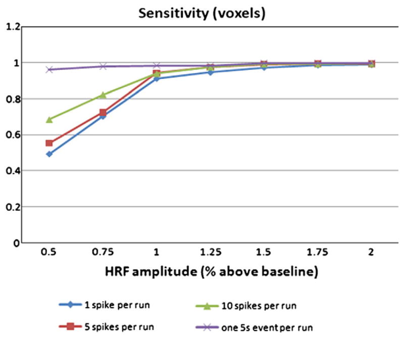
Sensitivity of the method in terms of well classified voxels for simulated data. For effective detection, an HRF amplitude of at least 1% above baseline was required, while an amplitude of 0.5% was sufficient for one 5 s event.

To conclude, although the method is not able to detect all activities in a time course, the spatio-temporal step allows to correctly gather voxels with the same simulated activity.

Patient data

Fifteen patients with focal epilepsy were selected. The functional data were acquired in series of 7–14 runs of 6 min each using a ${\text{T}}_2^{\ast }$-weighted EPI sequence. Although a patient has some runs with events, other runs can be without events. A patient was included if EEG–fMRI results showed clear activation and if some runs had few epileptic events (fewer than 5). The second criterion was used due to the sparsity constraint of our method. Only the patient runs with clear activation in their EEG–fMRI results were analyzed with our method. First, two groups of run were defined according to the number of events per run. For the first group, 28 runs with 1 to 5 events per run were selected. The second group was formed by 13 runs with more than 10 events per run. Second, the runs without any event from the 15 patients were selected for a third group (5 runs had no event).

Performance in detecting epileptic activity in patients

The method was evaluated by demonstrating its performance in comparison to EEG–fMRI (our “gold standard”) and 2D-TCA (“reference” method in the literature) (Khatamian et al., 2011), in detecting epileptic activity in patients. As in our simulation study, four clusters were used in the spatio-temporal clustering, but this time only the cluster corresponding to the sparsest mean component was retained. For the voxels inside this cluster, the maximum of detected activation in each voxel was used to generate an activation map.

First, the event detection sensitivity of the method was assessed by comparing the detected events with the events read on EEG. Table 1 shows this comparison, separating the first and second groups of runs, and showing the number of detected events considered as true positive and false positive. These numbers were measured on the mean component of the selected cluster. Fig. 5 shows an example of mean component obtained for a run. Four spikes were read on EEG by a neurologist in this run and the method detected two true positive and no false positive event. The method did not usually detect all the events in a run. In fact, 1.4±0.8 events for the first group and 2.0± 1.6 for the second group were detected on average, compared to 2.5± 1.2 and 14.4±3.0 events read on EEG for the first and second groups, respectively. Only 66% and 14% in average of EEG events were truly identified by our approach for the first and second groups, respectively. However, 26/28 and 11/13 runs had at least one concordant event for the first and second groups, respectively. Also, the method was very specific, because few of these runs had false positive events. The rightmost column of Table 1 reflects the delay of the hemody-namic response with the event read on EEG. It was computed by taking the timing of the maxima of true positive BOLD events and subtracting it from the timing of the corresponding events read on EEG (symbol Δ in Fig. 5). These measures showed important inter-and intra-variability between patients in the delay of the hemody-namic response. The mean value was around 6 s, which corresponds to the delay commonly used in fMRI analyses (see Fig. 6). In conclusion, the dilated and translated versions of the activelet were sufficient to account for HRF shape fluctuations. Indeed, Table 1 shows that the method was able to detect hemodynamic responses with different times to peak and shapes (spike or burst).

Table 1.

Comparison of events observed in EEG and events detected by our method. The rightmost column shows the time difference between the events observed in EEG and the events detected by our method in the BOLD signal.

Group #	Patient characteristics			Event detection by our method
	Patient #	Event type	# of events	True positive	False positive	Average time to peak±standard deviation (s)
1	1	Spike	4	2	0	4.2±0.8
	1	Spike	2	1	1	9.3±0.0
	2	Spike	2	1	0	7.5±0.0
	2	Spike	2	2	1	5.3±1.1
	3	Burst	1	1	0	8.7±0.0
	4	Spike	4	3	0	5.9±0.1
	5	Spike	4	2	0	7.6±1.6
	5	Spike	1	1	0	2.1±0.0
	6	Burst	2	2	0	7.3±1.3
	7	Spike	2	1	0	−0.6±0.0
	7	Spike	3	0	1
	8	Burst	2	1	1	7.3±0.0
	8	Burst	2	1	1	6.4±0.0
	9	Burst	3	3	0	5.2±2.9
	9	Burst	3	2	0	3.8±0.3
	9	Burst	2	2	0	2.1±0.8
	9	Burst	4	2	0	3.9±0.4
	10	Spike	3	2	0	3.3±0.6
	11	Spike	2	1	0	7.4±0.0
	11	Burst	1	1	0	8.7±0.0
	11	Burst	1	1	0	9.1±0.0
	12	Burst	5	2	0	4.6±1.4
	13	Spike	3	0	1
	13	Spike	2	1	0	5.1±0.0
	14	Burst	1	1	0	7.2±0.0
	15	Spike	5	3	0	6.4±2.9
	15	Spike	2	2	0	4.9±1.5
	15	Spike	3	1	0	3.7±0.0
2	3	Burst	12	4	0	8.4±2.1
	3	Burst	13	5	0	6.8±1.8
	3	Burst	11	1	0	6.5±0.0
	3	Spike	18	3	0	4.5±2.0
	3	Spike	12	2	2	4.6±1.0
	8	Burst	20	2	0	5.2±1.7
	8	Burst	12	0	1
	8	Burst	14	0	1
	9	Spike	11	1	1	8.0±0.0
	11	Spike	18	1	0	9.8±0.0
	12	Burst	16	2	0	5.3±0.8
	15	Spike	17	1	2	6.2±0.0
	15	Spike	13	4	0	4.7±0.8

Fig. 5.

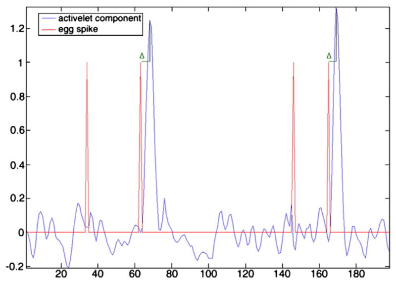
Example of mean component (blue line) extracted from voxels of selected cluster. The red line is the timings of interictal events read on EEG and the symbol Δ is the time delay between the EEG event and the BOLD response detected by the method.

Fig. 6.

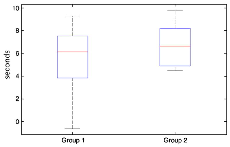
Box plot of delays between EEG events and BOLD changes detected by the method. This plot shows an average of 6.1 s and 6.7 s for the first and second groups, respectively. These values are close to the typical value used in fMRI analyses (around 6 s). Another important point is the variability of the delay.

The performance of our method in detecting activated regions close to EEG–fMRI analysis was then investigated. Results of 2D-TCA were also compared to EEG–fMRI analysis to evaluate our method with a reference method in the literature. 2D-TCA created many maps of activity with an average of 8 maps per subject for group 1 and 10 for group 2. Only runs in which 2D-TCA created a map that described what was seen by EEG–fMRI were reported and the most similar map to EEG–fMRI was selected. Table 2 summarizes the results. The maps obtained by our method were more similar to EEG–fMRI (with 26/28 and 9/13 significant positive correlations) than 2D-TCA (11/28 and 6/13 significant positive correlations) (Spearman’s test, P<0.05). The next validation was about the largest cluster of activity for the maps of each method. Although our method is not able to detect all events in a run, this detection is sufficient to get similarly activated regions compared to EEG–fMRI. The distance between centers of gravity of these two clusters showed no significant difference (P<0.05) for the first and second groups, while a most similar activity was found for the first group comparing our method to EEG–fMRI when measuring the distance between maxima voxels. It was also found that for the first group, our method and EEG–fMRI had similar sizes for their largest clusters, because a significant positive correlation was found between their largest clusters (R3=0.74, P<0.01) (Fig. 7). However, no significant positive correlation was found for the second group (R3=0.41, P=0.23), EEG–fMRI analysis creating maps with larger cluster size than our method. Figs. 8, 9, and 10 show examples of maps created by our method and EEG–fMRI. The location of maximum BOLD signal for the event detected by our method is displayed as a cross. Examples of strong correlation are shown in Figs. 8 and 9 and an example of no correlation is shown in Fig. 10. In this last example, a similar cluster of activity was found by both methods, but the largest clusters did not correspond.

Table 2.

Performance of our method in detecting activities close to EEG–fMRI analysis. The correlation between the maps obtained from EEG–fMRI and our method is shown in column 4. (+) means significant correlation (P<0.05). Columns 5, 6, 7 and 8 show the distances between centers of gravity and between maximum activation voxels for the most significant cluster obtained from “EEG–fMRI” and our method and “EEG–fMRI” and 2D-TCA method. Column 9 shows the number of components (t-maps) obtained from 2D-TCA method.

Group #	Patient characteristics			Our method results			2D-TCA results
	Patient #	Event type	# of events	Correlation of maps	Distance between centers of gravity (mm)	Distance between maxima (mm)	Distance between centers of gravity (mm)	Distance between maxima (mm)	# of components
1	1	Spike	4	0.41+	5	18	6	5	15
	1	Spike	2	0.02	20	42			7
	2	Spike	2	0.50+	9	5	5	11	11
	2	Spike	1	0.72+	4	7	23	9	11
	3	Burst	1	0.79+	6	29	5	16	13
	4	Spike	4	0.4+	20	11			5
	5	Spike	4	0.14+	19	31			4
	5	Spike	1	0.42+	17	5			2
	6	Burst	2	0.29+	15	41			14
	7	Spike	2	0.28+	6	17	10	16	12
	7	Spike	3	0.24+	16	16			6
	8	Burst	2	0.46+	10	29	12	15	12
	8	Burst	2	0.27+	9	38			4
	9	Burst	3	0.33+	12	9			13
	9	Burst	3	0.35+	38	22			11
	9	Burst	2	0.14+	15	32			8
	9	Burst	4	0.37+	32	25	33	24	8
	10	Spike	3	0.09+	9	11			4
	11	Spike	2	0.17+	11	34			3
	11	Burst	1	0.19+	20	15			5
	11	Burst	1	0.28+	8	50	14	8	9
	12	Burst	5	0.19+	13	15			10
	13	Spike	3	0.05	35	56			14
	13	Spike	2	0.32+	7	19	22	13	7
	14	Burst	1	0.41+	9	11	10	7	7
	15	Spike	5	0.29+	15	17			9
	15	Spike	2	0.44+	11	9			6
	15	Spike	3	0.29+	21	22	15	19	4
2	3	Burst	12	0.14+	17	12	15	8	14
	3	Burst	13	0.28+	46	79			12
	3	Burst	11	0.20+	9	32			8
	3	Spike	18	0.01	32	51	21	19	9
	3	Spike	12	0.24+	15	52			6
	8	Burst	20	−0.01	21	12			15
	8	Burst	12	0.14+	23	21			11
	8	Burst	14	0.04	25	31	19	18	10
	9	Spike	11	0.18+	19	29	22	13	11
	11	Spike	18	0.64+	12	35	19	9	13
	12	Burst	16	0.12+	21	31			8
	15	Spike	17	−0.06	45	62			9
	15	Spike	13	0.16+	23	28	21	19	9

Fig. 7.

Box plot of cluster sizes for first and second groups. For the first group, a significant positive correlation was found between the largest clusters of our method and EEG–fMRI (R3=0.74, P<0.01). However, no significant positive correlation was found for the second group (R3=0.41, P=0.23).

Fig. 8.

Example of high correlation between the maps created by (A) our method and (B) EEG–fMRI for the first group (patient #2 run #2 of Table 2).A strong correlation is found between our method and EEG–fMRI regarding the localization of the largest activation.

Fig. 9.

Example of high correlation between the maps created by (A) our method and (B) EEG–fMRI for the second group (patient #11 run #1 of Table 2).A strong correlation is found between our method and EEG–fMRI regarding the localization of the largest activation.

Fig. 10.

Example of no correlation between the maps created by (A) our method and (B) EEG–fMRI for the first group (patient #13 run #1 of Table 2).A similar cluster of activity was found by both methods, but the largest clusters did not correspond.

Finally, the last validation was to observe how the method works in the case of runs without event read on EEG. Three activity maps from 2 patients were concordant with the patient’s diagnostic and 2 activity maps had no concordance with the patient’s diagnostic. Fig. 11 shows an example of map in agreement with the patient’s diagnostic. The most significant activated cluster was observed in the left inferior frontal cortex. This activation fitted with one run for this patient and the localization of this spike fitted with some spikes found in long-term EEG monitoring. Moreover, a small spike was observed on scalp EEG in checking in a range of 10 s around the timing of events detected in fMRI. This spike was not marked by the neurologist due to its low amplitude, but its mapping was similar to the region detected in fMRI.

Fig. 11.

(top) fMRI activation obtained by the method for a run without spike on scalp EEG. fMRI shows a bilateral activation with a maximum over the left inferior frontal cortex. This activation fit with one run for this patient and the localization of this spike fit with some spikes found in long-term EEG monitoring. (bottom) Scalp EEG: few seconds around the timing of the activity detected in fMRI; the blue line shows a spike with low amplitude over the left fronto-temporal region which was not marked by the neurologist. The figures on the right show the mapping of the spike (top) and the mapping few milliseconds after the spike (bottom).

Discussion

EEG–fMRI has been shown to be clinically useful in the localization of epileptic discharges (Gotman, 2008). fMRI has also been shown to be potentially useful for localizing epileptic activity throughout the entire brain (Morgan et al., 2007). Our study proposes a new framework to localize epileptic activity in fMRI without dependence on the timing of events read on a simultaneously recorded EEG. The main benefit of this approach is to remove the issues related to recording the EEG inside the scanner and to be able to detect activity restricted to deep brain structures, which is unlikely to be detected by scalp EEG.

Proposed method

To address the problem of “blind” activity detection in fMRI, two kinds of approach can be used: the data-driven approach or the model-based approach. Data-driven approaches are the most commonly used. 2D-TCA detects transients in fMRI data independently of the EEG (Morgan et al., 2008) and the ICA approach decomposes fMRI data sets into spatially independent components (LeVan and Gotman, 2009). These techniques require estimating a priori the number of components or clusters and then selecting those corresponding to the epileptic activity. Otherwise, the methods create maps describing other activity not associated with epileptic discharges (Khatamian et al., 2011).

In this study, we proposed a combination of model-based and data-driven framework for the detection of epileptic activity in fMRI without recording the EEG. The method was based on a modeling of the HRF by wavelet decomposition. A new wavelet basis, called activelet, is able to model the HRF by assuming a linear approximation to the balloon model. This linearity is a common assumption in fMRI analysis. The benefit of this new wavelet basis is to model the HRF with few coefficients. For example, we needed 5 coefficients, on average, to reconstruct different shapes of HRF with a SNR of 30 dB, while we needed 30 coefficients with a traditional wavelet basis. This is why a sparse estimation technique was used to select wavelet coefficients corresponding to the presumed BOLD activity. In order to increase the specificity of the method, we decided to use the Homotopy algorithm (Donoho and Tsaig, 2008), because this iterative algorithm only selects one coefficient at each iteration. The Homotopy algorithm selected coefficients according to a dictionary (activelet decomposition for our study). A dictionary with only one activelet basis was sufficient to model the HRF for simulated and real data. The dilated and translated versions of the activelet basis were able to capture different shapes of HRF, but other activelet basis could be added to the dictionary in modifying the balloon parameters in the definition of vector α⃗ and scalar γ (Fig. 2) (Friston et al., 2000).

Finally, during this stage of epileptic activity detection for each time course, we are not taking into account the physiological noise. An automatic method could be used to remove this noise from the data to achieve structured noise reduction and improve the detection of signal fluctuations related to neuronal activity (Perlbarg et al., 2007).

Comparison with methods from the literature

Model-based approaches have been developed to analyze data with no timing constraints (Faisan et al., 2007; Hutchinson et al., 2009). A recent study proposed a method based on the mathematical deconvolution of the HRF from the time courses and a temporal t-statistics to detect activity timings in the deconvolved signal (Gaudes et al., 2010). The method was validated on five subjects who performed visually cued finger tapping at 7 T. However, this method needs a baseline period to evaluate the statistical significance of the activations and this period has to be sufficiently long to properly estimate the mean amplitude and variance of the baseline state. This kind of statistics is difficult in the case of epilepsy due to the difficulty to define a baseline period. Moreover, this is impossible in the case of runs with lots of spikes, because the number of time point for this period has to be large enough (>30) and of sufficient length (>60 s). In our study, variable shapes of HRF can be captured by the activelet dictionary compared to a deconvolution framework. Also, we used a clustering stage to gather voxels according to timings of detected activations and spatial information, instead of a statistical test to detect activated voxels.

Perspectives of the method

In this study, we are interested in “blind deconvolution” in the wavelet domain. However, other approaches can be used. One possibility is to model the timing of the events as a Bernoulli process, while their magnitudes are statistically modeled by a Gaussian distribution (Champagnat et al., 1996). In this context, recent studies based on efficient Bayesian extensions could be used to simultaneously estimate the hemodynamic response function and the input spike train signal (Ge et al., 2011a, 2011b).

The method used in this study was a univariate analysis as the detection of epileptic events was based on a voxelwise estimation. The use of multivariate analysis could improve the sensitivity of this detection. The first approach will be to extend the method to perform spatially regularized detection of epileptic events. This could be addressed by combining sparsity in the activelets domain and spatial regularization in the image domain. The second approach would be to combine the two stages of the method in a joint framework. In this context, the work of Lu et al. (2007) gives some interesting directions.

Simulated data

The method was evaluated on simulated and real data. Various characteristics of epileptic activity were studied in our simulations (size of simulated regions – shape of the HRF – amplitude of the simulated events – number of events per run). The range of HRF amplitudes from 0.5 to 2% above baseline corresponded to typical values in realistic fMRI data (Gu et al., 2001). A maximal rate of 10 spikes per run was used in the simulations and the artificial time courses were generated in a way that preserved the linearity of the response. The method was dependent on the amplitude and the kind of event but not on the size of the simulated region and the shape of the HRF. An amplitude of at least 1% was necessary for the spikes, while the method was efficient in almost all test cases for a long event (5 s). The successful detection of 5 s events showed that the method could work well for short seizures. Simulations cannot reproduce all the conditions present in real data, but they still provide a controlled way of evaluating the performance of the method under realistic parameters and also a way to define some degrees of freedom of a method, such as the number of scales in the activelet decomposition (3 scales in our study) and the vector α⃗ and the scalar γ in the activelets definition (Eq. (3)).

Comparison with EEG–fMRI

The second validation was on real data. 15 epileptic patients were selected according to their results in EEG–fMRI and the number of events per run. We decided to select the patients with clear activation in EEG–fMRI, because this technique was considered as our “gold-standard”. The number of events was also an important criterion because our method is supposed to be more efficient in the case of rare events, due to the sparsity constraint. Firstly, the results of our method and EEG–fMRI analysis were compared in terms of correlation between the two maps. A threshold value corresponding to a P-value of 0.05 corrected for multiple comparisons and spatial extent was applied to the statistical t-map obtained from EEG–fMRI. The two maps were binarized and a correlation coefficient was computed between the two maps. The second measure for the comparison of the two methods was based on the most significant cluster obtained from each method. We measured the distances between both the centers of gravity and the maxima voxels. It is difficult to define a method of validation in fMRI analysis, but in most fMRI studies, the most significant cluster and the maxima voxel are common measures. The results suggested that the method was more efficient in the case of runs with few events than with many events. Our method was able to find the same maps of activity as EEG–fMRI analysis in the majority of runs.

Our method has several advantages compared to EEG–fMRI. EEG–fMRI has a lack of sensitivity in the case of patients with too few spikes, due to statistical issues, while our framework is suitable for the assessment of these patients due to sparsity constraint. In addition, EEG–fMRI analyses are optimal if the modeling assumptions are correct. These techniques commonly employ a canonical HRF shape, sometimes with multiple delays (Bagshaw et al., 2004), or more flexible basis sets to model arbitrary HRF shapes (Josephs and Henson, 1999; Lu et al., 2006). However, these models do not account for inter-trial variability in the delay of the HRF and the last column of Table 1 shows some inter-run variability in terms of time to peak (see the standard deviation). In the case of one run for instance, we observed that the BOLD response preceded the spike on the EEG. This phenomenon has been observed in focal and generalized epilepsy (Hawco et al., 2007; Jacobs et al., 2009; Moeller et al., 2008), but our method is insensitive to it. The quality of the EEG recording inside the scanner is also an important factor. Strong artifacts are visible on scalp EEG (such as gradient artifact and ballistocardiogram). Although techniques have been developed to remove these artifacts (Benar et al., 2003), this is sometimes very difficult. Moreover, our method has the potential to detect activity restricted to deep brain structures since the HRF is independent of brain localization, unlike the EEG. While this was evident when our method was applied to simulated data (i.e. detection of the activity in the hippocampal VOI), it was not confirmed in patient data. Finally, our approach seemed to work for some runs without epileptic events visible on scalp EEG. A perspective will be to compare the focus of activation obtained by our approach with other information, such as intracranial EEG, long-term EEG recording, imaging findings and the patient’s final diagnosis.

Comparison with 2D-TCA method

We also investigated the performance of our method in detecting epileptic activity as compared to 2D-TCA. 2D-TCA was chosen because it is the only method used for the detection of epileptic activity in fMRI without EEG co-registration (Khatamian et al., 2011; Morgan et al., 2007); it has also a better performance than ICA (Morgan et al., 2008). Compared with 2D-TCA, our method had better sensitivity and specificity. 2D-TCA created maps describing other activity not associated with epilepsy, while only one map of activity was created with our method. The amplitude threshold used to detect activity in each time course can explain the lack of sensitivity and specificity of 2D-TCA.

Conclusion

We propose a framework for the detection of epileptic activity in fMRI without recording the EEG. The validity of this method was tested by a simulation study and real fMRI data (15 patients with focal epilepsy). The results showed that the new algorithm could identify the regions corresponding to epileptic activity, especially for patients with few events but also in some patients with frequent spikes. It may therefore be possible, at least when spikes are infrequent, to detect their BOLD manifestations without having to record the EEG in the scanner. A prior EEG may be used to assess the likelihood that spikes are rare. However, this framework needs more investigation for patients without clear activation in EEG–fMRI. In this study, the patients were selected if EEG–fMRI gave clear activation in concordance with the patient’s diagnostic. This means that the hemodynamic response must have been large in order to have clear activation with EEG–fMRI despite rare events. After this second validation is completed, studies similar to those performed with EEG–fMRI may be extended to fMRI alone and may also include patients with infrequent epileptic events, ultimately improving non-invasively the localization of the epileptic focus.

Appendix A. Biophysical models of fMRI responses and activelets design

The designing of activelets basis is based on the biophysical model of Friston et al. (2000). This model comprises one input (the stimulus u), four hemodynamic state variables {s, f_in, v, q}, whose interactions are described by differential equations with seven hemodynamic parameters. These parameters have an explicit biophysical meaning (see Table A.1). For the state variables, s is the flow inducing signal, f_in the blood flow, v the normalized venous volume and q the normalized deoxy-hemoglobin content. The system of the hemodynamic model is defined by:

$$\{\begin{array}{c}\stackrel{.}{s}=\in \text{u}-\frac{\text{s}}{{\tau }_{\text{s}}}-\frac{{\text{f}}_{\text{in}}-1}{{\tau }_{\text{f}}}\\ {\stackrel{.}{f}}_{\text{in}}=\text{s}\\ \stackrel{.}{v}=\frac{1}{{\tau }_0}\left({\text{f}}_{\text{in}}-{\text{v}}^{\frac{1}{\alpha }}\right)\\ \stackrel{.}{q}=\frac{1}{{\tau }_0}\left({\text{f}}_{\text{in}}\frac{1-{(1-{\text{E}}_0)}^{\frac{1}{{\text{f}}_{\text{in}}}}}{{\text{E}}_0}-{\text{v}}^{\frac{1}{\alpha }-1}\text{q}\right).\end{array}$$ (A.1)

And one observed quantity (the BOLD signal):

$${\text{BOLD}}_{\text{non}-\text{linear}}={\text{V}}_0\left({\text{k}}_1(1-\text{q})+{\text{k}}_2\left(1-\frac{\text{q}}{\text{v}}\right)+{\text{k}}_3(1-\text{v})\right).$$ (A.2)

From a linear approximation of Eqs. (A.1) and (A.2) Khalidov et al. (2011) obtain a linear differential equation of the form:

$$\left({\text{D}}^4+{\text{a}}_3{\text{D}}^3+{\text{a}}_2{\text{D}}^2+{\text{a}}_1\text{D}+{\text{a}}_0\right)\text{y}=(\text{D}-\gamma )\text{x}.$$ (A.3)

Where x(t) is a neuronal input signal, y(t) is the linear BOLD response and D is the first order differential operator.

If we denote the operator L such as Ly=x, then the hemodynamic response h(t) is given by:

$$\text{L}\{\text{h}(\text{t})\}=\delta (\text{t}).$$ (A.4)

Where δ(t) denotes the Dirac impulse.

Mathematically, h(t) is thus a Green function of L and:

$$\text{h}(\text{t})={\mathcal{L}}^{-1}\left\{\frac{(.-\gamma )}{{\prod }_{\text{n}=1}^4(.-{\alpha }_{\text{n}})}\right\}(\text{t}).$$ (A.5)

Where, is the inverse Laplace transform and α = (α₁, …, α_N) the roots of the polynomial s⁴ + a₃s³ + a₂s² + a₁s + a₀.

In our case, α⃗ and γ are defined by identifying the operator L that is linked to the hemodynamic system by using a linear approximation of the expanded balloon model (see Eq. (A.3)):

$$\begin{array}{l}\overrightarrow{\mathit{\alpha }}=\left(-\frac{1}{0},-\frac{1}{0},-\frac{1}{2_{\text{s}}}\left(1\pm \text{j}\sqrt{\frac{4{\tau }_{\text{s}}^2}{{\tau }_{\text{f}}}-1}\right)\right)\\ \mathit{\gamma }=\left(-\frac{({\text{k}}_1+{\text{k}}_2)\left(\frac{1-\alpha }{\alpha {\tau }_0}-\frac{\text{c}}{\alpha }\right)-({\text{k}}_3-{\text{k}}_2)\frac{1}{{\tau }_0}}{-({\text{k}}_1+{\text{k}}_2)\text{c}{\tau }_0-{\text{k}}_3+{\text{k}}_2}\right).\end{array}$$ (A.6)

With $\text{c}=\frac{1+(1-{\text{E}}_0)ln(1-{\text{E}}_0)/{\text{E}}_0}{{\tau }_0}$. Given a smoothing function ϕ (also called basis functions, see Khalidov et al. (2011)) at some scale j and localized at time t=k2^j, the wavelet coefficient of some BOLD response b(t) is defined by:

$$\langle \text{b},{\mathrm{\Psi }}_{\text{j}}(.-\text{t})\rangle =\text{L}\left\{\text{b}\right\}\ast {\mathrm{\phi }}_{\text{j}}(\text{t}).$$ (A.7)

Where Ψ_j are the wavelet functions at a different scale j.

Activelets generate a generalized multiresolution analysis that is non-stationary in the sense that the wavelets and the scaling functions depend on the scale. Fast Mallat’s filterbank algorithm with scale dependent filters is used to perform the decomposition and the reconstruction in this new wavelet basis (see Khalidov et al. (2011) for details about implementation).

Appendix B. Homotopy algorithm

The Homotopy method (Donoho and Tsaig, 2008) was used to solve Eq. (4). The algorithm starts out at β_in =0 and λ = ||Φ^Ty||_¥, and iteratively builds a sparse solution by adding or removing elements from the solution set (called “active set” in the literature). The solution path is followed by keeping the optimality conditions of Eq. (4) at each point along the path. This method is very favorable in a sparse setting, because it will reach the solution in few steps when the solution has few nonzero. The regularization parameter λ controls the sparsity of β, when λ decreases, the sparsity of the solution decreases, too. During this algorithm, the scaling and wavelet functions are normalized to have their l2-norm equal to 1, as required by the Homotopy algorithm.

Appendix C. Clustering algorithm

Firstly, a graph is constructed by connecting each vertex (voxels) in terms of functional and spatial distances. The exponential of Eq. (4) was used to transform d_i,j into a consistent similarity measure:

$${\text{W}}_{\text{i},\text{j}}={\text{e}}^{-{\text{d}}_{\text{i},\text{j}}}.$$ (C.1)

Eq. (C.1) corresponds to the standard Gaussian kernel often used in spectral clustering and the affinity matrix can be defined:

$${\text{S}}_{\text{i},\text{j}}=\{\begin{array}{cc}{\text{W}}_{\text{i},\text{j}}& \text{i}\ne \text{j}\\ 0& \text{i}=\text{j}\end{array}.$$ (C.2)

Then, the graph was clustered in a number of subsets consisting of group voxels that showed similar distances in terms of functional and spatial distances. This clustering step can be seen as a graph partitioning problem that wants to separate the vertices (voxels) of the graph into subsets (clusters) by eliminating edges connecting the subsets. The normalized cut graph clustering method of Shi and Malik (2000) was used, its aim being to normalize the cut cost by the fraction of all paths in that subset. It has the strong advantage of being less sensitive to outliers than other graph clustering methods due to this normalization factor. Thus, this method measures both the dissociation between clusters as well as the affinities within a cluster. The eigenvectors of the normalized Laplacian matrix D^−1/2SD (with D is the diagonal matrix, D_ii = Σ_jS_ij) were computed to optimize normalized cut objective function by using the spectral graph theory (Chung, 1997).

Table A.1.

List of the hemodynamic parameters involved in the activelets, with their meaning and their common values.

Constant	Meaning	Value [REF]
τ0	Transit time	0.54
α	Balloon stiffness	0.33
τs	Signal decay	1.54
τf	Autoregulation	2.46
E0	Oxygen extraction fraction	0.34
k1	BOLD constant 1	7E0
k2	BOLD constant 2	2
k3	BOLD constant 3	2E0–0.2

Finally, the eigenvectors can be used to map the voxels into a new space and the use of k-means clustering allows getting the clusters of voxels (Shi and Malik, 2000).

References

- Aghakhani Y, Bagshaw AP, Benar CG, Hawco C, Andermann F, Dubeau F, Gotman J. fMRI activation during spike and wave discharges in idiopathic generalized epilepsy. Brain. 2004;127 (Pt 5):1127–1144. doi: 10.1093/brain/awh136. [DOI] [PubMed] [Google Scholar]
- Allen PJ, Josephs O, Turner R. A method for removing imaging artifact from continuous EEG recorded during functional MRI. Neuroimage. 2000;12 (2):230–239. doi: 10.1006/nimg.2000.0599. [DOI] [PubMed] [Google Scholar]
- Bagshaw AP, Aghakhani Y, Benar CG, Kobayashi E, Hawco C, Dubeau F, Pike GB, Gotman J. EEG–fMRI of focal epileptic spikes: analysis with multiple haemo-dynamic functions and comparison with gadolinium-enhanced MR angiograms. Hum Brain Mapp. 2004;22 (3):179–192. doi: 10.1002/hbm.20024. [DOI] [PMC free article] [PubMed] [Google Scholar]
- Bagshaw AP, Hawco C, Benar CG, Kobayashi E, Aghakhani Y, Dubeau F, Pike GB, Gotman J. Analysis of the EEG–fMRI response to prolonged bursts of inter-ictal epileptiform activity. Neuroimage. 2005;24 (4):1099–1112. doi: 10.1016/j.neuroimage.2004.10.010. [DOI] [PubMed] [Google Scholar]
- Baumgartner R, Ryner L, Richter W, Summers R, Jarmasz M, Somorjai R. Comparison of two exploratory data analysis methods for fMRI: fuzzy clustering vs. principal component analysis. Magn Reson Imaging. 2000;18 (1):89–94. doi: 10.1016/s0730-725x(99)00102-2. [DOI] [PubMed] [Google Scholar]
- Beckmann CF, Smith SM. Probabilistic independent component analysis for functional magnetic resonance imaging. IEEE Trans Med Imaging. 2004;23 (2):137–152. doi: 10.1109/TMI.2003.822821. [DOI] [PubMed] [Google Scholar]
- Benar CG, Gross DW, Wang Y, Petre V, Pike B, Dubeau F, Gotman J. The BOLD response to interictal epileptiform discharges. Neuroimage. 2002;17 (3):1182–1192. doi: 10.1006/nimg.2002.1164. [DOI] [PubMed] [Google Scholar]
- Benar C, Aghakhani Y, Wang Y, Izenberg A, Al-Asmi A, Dubeau F, Gotman J. Quality of EEG in simultaneous EEG–fMRI for epilepsy. Clin Neurophysiol. 2003;114 (3):569–580. doi: 10.1016/s1388-2457(02)00383-8. [DOI] [PubMed] [Google Scholar]
- Buxton RB, Wong EC, Frank LR. Dynamics of blood flow and oxygenation changes during brain activation: the balloon model. Magn Reson Med. 1998;39 (6):855–864. doi: 10.1002/mrm.1910390602. [DOI] [PubMed] [Google Scholar]
- Champagnat F, Goussard Y, Idier J. Unsupervised deconvolution of sparse spike trains using stochastic approximation. IEEE Trans Signal Process. 1996;44 (12):2988–2998. [Google Scholar]
- Chung FRK, editor. American Mathematical Society, editor Spectral Graph Theory. 1997. [Google Scholar]
- Crouse MS, Nowak RD, Baraniuk RG. Wavelet-based statistical signal processing using hidden Markov models. IEEE Trans Signal Process. 1998;46 (4):886–902. [Google Scholar]
- Donoho DL, Johnstone IM. Ideal spatial adaptation by wavelet shrinkage. Bio-metrika. 1994;81 (3):425–455. [Google Scholar]
- Donoho DL, Tsaig Y. Fast solution of l1-norm minimization problems when the solution may be sparse. IEEE Trans Inf Theory. 2008;54 (11):4789–4812. [Google Scholar]
- Fadili MJ, Ruan S, Bloyet D, Mazoyer B. A multistep unsupervised fuzzy clustering analysis of fMRI time series. Hum Brain Mapp. 2000;10 (4):160–178. doi: 10.1002/1097-0193(200008)10:4<160::AID-HBM20>3.0.CO;2-U. [DOI] [PMC free article] [PubMed] [Google Scholar]
- Faisan S, Thoraval L, Armspach JP, Heitz F. Hidden Markov multiple event sequence models: a paradigm for the spatio-temporal analysis of fMRI data. Med Image Anal. 2007;11 (1):1–20. doi: 10.1016/j.media.2006.09.003. [DOI] [PubMed] [Google Scholar]
- Friston KJ, Mechelli A, Turner R, Price CJ. Nonlinear responses in fMRI: the balloon model, Volterra kernels, and other hemodynamics. Neuroimage. 2000;12 (4):466–477. doi: 10.1006/nimg.2000.0630. [DOI] [PubMed] [Google Scholar]
- Gaudes CC, Petridou N, Dryden IL, Bai L, Francis ST, Gowland PA. Detection and characterization of single trial fMRI bold responses: paradigm free mapping. Hum Brain Mapp. 2010;32 (9):1400–1418. doi: 10.1002/hbm.21116. [DOI] [PMC free article] [PubMed] [Google Scholar]
- Ge D, Idier J, Le Carpentier E. Enhanced sampling schemes for MCMC based blind Bernoulli–Gaussian deconvolution. Signal Process. 2011a;91 (4):759–772. [Google Scholar]
- Ge D, Le Carpentier E, Idier J, Farina D. Spike sorting by stochastic simulation. IEEE Trans Neural Syst Rehabil Eng. 2011b;19 (3):249–259. doi: 10.1109/TNSRE.2011.2112780. [DOI] [PMC free article] [PubMed] [Google Scholar]
- Glover GH. Deconvolution of impulse response in event-related BOLD fMRI. Neuroimage. 1999;9 (4):416–429. doi: 10.1006/nimg.1998.0419. [DOI] [PubMed] [Google Scholar]
- Gotman J. Epileptic networks studied with EEG–fMRI. Epilepsia. 2008;49 (Suppl 3):42–51. doi: 10.1111/j.1528-1167.2008.01509.x. [DOI] [PMC free article] [PubMed] [Google Scholar]
- Goutte C, Hansen LK, Liptrot MG, Rostrup E. Feature-space clustering for fMRI meta-analysis. Hum Brain Mapp. 2001;13 (3):165–183. doi: 10.1002/hbm.1031. [DOI] [PMC free article] [PubMed] [Google Scholar]
- Gu H, Engelien W, Feng H, Silbersweig DA, Stern E, Yang Y. Mapping transient, randomly occurring neuropsychological events using independent component analysis. Neuroimage. 2001;14 (6):1432–1443. doi: 10.1006/nimg.2001.0914. [DOI] [PubMed] [Google Scholar]
- Hawco CS, Bagshaw AP, Lu Y, Dubeau F, Gotman J. BOLD changes occur prior to epileptic spikes seen on scalp EEG. Neuroimage. 2007;35 (4):1450–1458. doi: 10.1016/j.neuroimage.2006.12.042. [DOI] [PubMed] [Google Scholar]
- Hutchinson RA, Niculescu RS, Keller TA, Rustandi I, Mitchell TM. Modeling fMRI data generated by overlapping cognitive processes with unknown onsets using Hidden Process Models. Neuroimage. 2009;46 (1):87–104. doi: 10.1016/j.neuroimage.2009.01.025. [DOI] [PubMed] [Google Scholar]
- Jacobs J, Levan P, Moeller F, Boor R, Stephani U, Gotman J, Siniatchkin M. Hemodynamic changes preceding the interictal EEG spike in patients with focal epilepsy investigated using simultaneous EEG–fMRI. Neuroimage. 2009;45 (4):1220–1231. doi: 10.1016/j.neuroimage.2009.01.014. [DOI] [PubMed] [Google Scholar]
- Josephs O, Henson RN. Event-related functional magnetic resonance imaging: modelling, inference and optimization. Philos Trans R Soc Lond B Biol Sci. 1999;354 (1387):1215–1228. doi: 10.1098/rstb.1999.0475. [DOI] [PMC free article] [PubMed] [Google Scholar]
- Khalidov I. PhD Thesis. Lausanne: Ecole polytechnique federale; 2009. Operator-like wavelets with application to functional magnetic resonance imaging; p. 119. [Google Scholar]
- Khalidov I, Fadili MJ, Lazeyras F, Van De Ville D, Unser M. Activelets: wavelets for sparse representation of hemodynamic responses. Signal Process. 2011;91 (12):2810–2821. [Google Scholar]
- Khatamian YB, Fahoum F, Gotman J. Limits of 2D-TCA in detecting BOLD responses to epileptic activity. Epilepsy Res. 2011;94 (3):177–188. doi: 10.1016/j.eplepsyres.2011.01.018. [DOI] [PMC free article] [PubMed] [Google Scholar]
- Kobayashi E, Bagshaw AP, Benar CG, Aghakhani Y, Andermann F, Dubeau F, Gotman J. Temporal and extratemporal BOLD responses to temporal lobe interictal spikes. Epilepsia. 2006;47 (2):343–354. doi: 10.1111/j.1528-1167.2006.00427.x. [DOI] [PubMed] [Google Scholar]
- LeVan P, Gotman J. Independent component analysis as a model-free approach for the detection of BOLD changes related to epileptic spikes: a simulation study. Hum Brain Mapp. 2009;30 (7):2021–2031. doi: 10.1002/hbm.20647. [DOI] [PMC free article] [PubMed] [Google Scholar]
- Lindquist MA, Wager TD. Validity and power in hemodynamic response modeling: a comparison study and a new approach. Hum Brain Mapp. 2007;28 (8):764–784. doi: 10.1002/hbm.20310. [DOI] [PMC free article] [PubMed] [Google Scholar]
- Lu Y, Bagshaw AP, Grova C, Kobayashi E, Dubeau F, Gotman J. Using voxel-specific hemodynamic response function in EEG–fMRI data analysis. Neuroimage. 2006;32 (1):238–247. doi: 10.1016/j.neuroimage.2005.11.040. [DOI] [PubMed] [Google Scholar]
- Lu Y, Grova C, Kobayashi E, Dubeau F, Gotman J. Using voxel-specific hemo-dynamic response function in EEG–fMRI data analysis: an estimation and detection model. Neuroimage. 2007;34 (1):195–203. doi: 10.1016/j.neuroimage.2006.08.023. [DOI] [PubMed] [Google Scholar]
- Makni S, Idier J, Vincent T, Thirion B, Dehaene-Lambertz G, Ciuciu P. A fully Bayesian approach to the parcel-based detection-estimation of brain activity in fMRI. Neuroimage. 2008;41 (3):941–969. doi: 10.1016/j.neuroimage.2008.02.017. [DOI] [PubMed] [Google Scholar]
- Mandeville JB, Marota JJ, Ayata C, Zaharchuk G, Moskowitz MA, Rosen BR, Weisskoff RM. Evidence of a cerebrovascular postarteriole windkessel with delayed compliance. J Cereb Blood Flow Metab. 1999;19 (6):679–689. doi: 10.1097/00004647-199906000-00012. [DOI] [PubMed] [Google Scholar]
- Moeller F, Siebner HR, Wolff S, Muhle H, Boor R, Granert O, Jansen O, Stephani U, Siniatchkin M. Changes in activity of striato-thalamo-cortical network precede generalized spike wave discharges. Neuroimage. 2008;39 (4):1839–1849. doi: 10.1016/j.neuroimage.2007.10.058. [DOI] [PubMed] [Google Scholar]
- Morgan VL, Price RR, Arain A, Modur P, Abou-Khalil B. Resting functional MRI with temporal clustering analysis for localization of epileptic activity without EEG. Neuroimage. 2004;21 (1):473–481. doi: 10.1016/j.neuroimage.2003.08.031. [DOI] [PubMed] [Google Scholar]
- Morgan VL, Gore JC, Abou-Khalil B. Cluster analysis detection of functional MRI activity in temporal lobe epilepsy. Epilepsy Res. 2007;76 (1):22–33. doi: 10.1016/j.eplepsyres.2007.06.008. [DOI] [PMC free article] [PubMed] [Google Scholar]
- Morgan VL, Li Y, Abou-Khalil B, Gore JC. Development of 2dTCA for the detection of irregular, transient BOLD activity. Hum Brain Mapp. 2008;29 (1):57–69. doi: 10.1002/hbm.20362. [DOI] [PMC free article] [PubMed] [Google Scholar]
- Perlbarg V, Bellec P, Anton JL, Pelegrini-Issac M, Doyon J, Benali H. CORSI-CA: correction of structured noise in fMRI by automatic identification of ICA components. Magn Reson Imaging. 2007;25 (1):35–46. doi: 10.1016/j.mri.2006.09.042. [DOI] [PubMed] [Google Scholar]
- Salek-Haddadi A, Diehl B, Hamandi K, Merschhemke M, Liston A, Friston K, Duncan JS, Fish DR, Lemieux L. Hemodynamic correlates of epileptiform discharges: an EEG–fMRI study of 63 patients with focal epilepsy. Brain Res. 2006;1088 (1):148–166. doi: 10.1016/j.brainres.2006.02.098. [DOI] [PubMed] [Google Scholar]
- Shen X, Papademetris X, Constable RT. Graph-theory based parcellation of functional subunits in the brain from resting-state fMRI data. Neuroimage. 2010;50 (3):1027–1035. doi: 10.1016/j.neuroimage.2009.12.119. [DOI] [PMC free article] [PubMed] [Google Scholar]
- Shi J, Malik J. Normalized cuts and image segmentation. IEEE Trans Pattern Anal Mach Intell. 2000;22 (8):888–905. [Google Scholar]
- Tyvaert L, Hawco C, Kobayashi E, LeVan P, Dubeau F, Gotman J. Different structures involved during ictal and interictal epileptic activity in malformations of cortical development: an EEG–fMRI study. Brain. 2008;131 (Pt 8):2042–2060. doi: 10.1093/brain/awn145. [DOI] [PMC free article] [PubMed] [Google Scholar]
- Varoquaux G, Sadaghiani S, Pinel P, Kleinschmidt A, Poline JB, Thirion B. A group model for stable multi-subject ICA on fMRI datasets. Neuroimage. 2010;51 (1):288–299. doi: 10.1016/j.neuroimage.2010.02.010. [DOI] [PubMed] [Google Scholar]
- Woolrich MW, Jenkinson M, Brady JM, Smith SM. Fully Bayesian spatio-temporal modeling of FMRI data. IEEE Trans Med Imaging. 2004;23 (2):213–231. doi: 10.1109/TMI.2003.823065. [DOI] [PubMed] [Google Scholar]
- Worsley KJ, Liao CH, Aston J, Petre V, Duncan GH, Morales F, Evans AC. A general statistical analysis for fMRI data. Neuroimage. 2002;15 (1):1–15. doi: 10.1006/nimg.2001.0933. [DOI] [PubMed] [Google Scholar]
- Zijlmans M, Huiskamp G, Hersevoort M, Seppenwoolde JH, van Huffelen AC, Leijten FS. EEG–fMRI in the preoperative work-up for epilepsy surgery. Brain. 2007;130:2343–2353. doi: 10.1093/brain/awm141. [DOI] [PubMed] [Google Scholar]