Leveraging reads that span multiple single nucleotide polymorphisms for haplotype inference from sequencing data

Abstract

Motivation: Haplotypes, defined as the sequence of alleles on one chromosome, are crucial for many genetic analyses. As experimental determination of haplotypes is extremely expensive, haplotypes are traditionally inferred using computational approaches from genotype data, i.e. the mixture of the genetic information from both haplotypes. Best performing approaches for haplotype inference rely on Hidden Markov Models, with the underlying assumption that the haplotypes of a given individual can be represented as a mosaic of segments from other haplotypes in the same population. Such algorithms use this model to predict the most likely haplotypes that explain the observed genotype data conditional on reference panel of haplotypes. With rapid advances in short read sequencing technologies, sequencing is quickly establishing as a powerful approach for collecting genetic variation information. As opposed to traditional genotyping-array technologies that independently call genotypes at polymorphic sites, short read sequencing often collects haplotypic information; a read spanning more than one polymorphic locus (multi-single nucleotide polymorphic read) contains information on the haplotype from which the read originates. However, this information is generally ignored in existing approaches for haplotype phasing and genotype-calling from short read data.

Results: In this article, we propose a novel framework for haplotype inference from short read sequencing that leverages multi-single nucleotide polymorphic reads together with a reference panel of haplotypes. The basis of our approach is a new probabilistic model that finds the most likely haplotype segments from the reference panel to explain the short read sequencing data for a given individual. We devised an efficient sampling method within a probabilistic model to achieve superior performance than existing methods. Using simulated sequencing reads from real individual genotypes in the HapMap data and the 1000 Genomes projects, we show that our method is highly accurate and computationally efficient. Our haplotype predictions improve accuracy over the basic haplotype copying model by ∼20% with comparable computational time, and over another recently proposed approach Hap-SeqX by ∼10% with significantly reduced computational time and memory usage.

Availability: Publicly available software is available at http://genetics.cs.ucla.edu/harsh

Contact: bpasaniuc@mednet.ucla.edu or eeskin@cs.ucla.edu

1 INTRODUCTION

Humans are diploid organisms with two copies of each chromosome, one inherited from the father and the other from the mother. The two copies are similar to each other and only differ at a small fraction () of sites. Most of the variation is contained at single nucleotide polymorphic (SNP) sites. The sequence of alleles on each chromosome is referred to as the haplotype. Haplotype information is centrally important for a wide variety of applications, including association studies and ancestry inference (Fearnhead and Donnelly, 2001; Hugot et al., 2001; Lazzeroni, 2001; Myers and Griffiths, 2003; Rioux et al., 2001; Sabeti et al., 2002). Unfortunately, standard methods for probing genetic variation are able to collect only genotype information but not haplotypes. A large number of computational methods, referred to as haplotype phasing approaches, have been proposed to infer haplotypes from genotypes. The most successful methods use a set of reference haplotypes to build a probabilistic model of the haplotypes in the population (Howie et al., 2009; Howie et al., 2011; Kang et al., 2010; Li et al., 2010; Long et al., 2009). Using a population genetics model for the haplotype distribution, these models predict the most likely haplotype data that can explain the observed genotypes.

Rapid advances in high-throughput sequencing (HTS) technologies provide new opportunities for haplotype phasing methods. HTS yields short segments of the DNA (reads) where each read originates from one of the pair of chromosomes. Therefore, all the alleles in this read are from the same haplotype. Although reads that cover multiple SNPs (multi-SNP reads) could be used to improve haplotype inference, existing methods generally ignore this information, partially owing to computational difficulty associated with modeling such reads.

Several methods have been proposed to predict haplotypes directly from the reads. These methods, referred to as haplotype assembly methods, use overlapping reads to construct the haplotype (Aguiar and Istrail, 2012; Bansal and Bafna, 2008; Bansal et al., 2008; Duitama et al., 2010, 2012; He et al., 2010; Xie et al., 2012). The most commonly used objective function for haplotype assembly is the minimum error correction (MEC). The MEC objective function aims at finding the minimum number of edits such that the reads can be partitioned into two disjoint sets, and each set of reads originates from one of the haplotypes. However, as these methods do not use the information in the reference haplotype panel, they significantly underperform standard phasing methods that ignore read information but use reference panel (He et al., 2010). Recently, one of these methods has been extended to use the reference (He and Eskin, 2013; He et al., 2012). Unfortunately, this method has prohibitive memory and time requirements, thus making it unfeasible for moderate to large datasets.

Here, we propose a novel approach called Haplotyping with Reference and Sequencing technology (HARSH) for haplotype phasing. We use a probabilistic model to incorporate the multi-SNP read information together with a reference panel of haplotypes. We use an efficient Gibbs sampling method to find sample from the posterior distribution. This algorithm has the advantages of being computationally efficient, scalable in memory usage and accurate in genotyping and phasing prediction. We evaluate our method on simulations from real haplotypes from the HapMap project. At 1× coverage, HARSH gives ∼10% improvement in terms of total error rate compared with standard phasing approaches that do not use the multi-SNP read information, thus showing the benefits of modeling multi-SNP reads. We also evaluate HARSH and the basic model for varying coverage and read length, showing the benefits of our approach in higher coverage and longer read length. Additionally, we test our method on simulations starting from real sequencing data of 1000 Genomes project, where the density of SNPs is much higher than that in HapMap data. Through extensive simulations we show that the gain in performance of our approach over existing models extends to realistic read lengths (e.g. 100–400 bp), making our approach readily applicable to existing sequencing datasets. With recent works showing that short read sequencing can dramatically increase association power in genome-wide association study over genotyping arrays (Pasaniuc et al., 2012), we expect our approaches to further increase power in genome-wide association study by increasing accuracy in genotype calling and phasing from short read data.

2 METHODS

The best performing approaches for haplotype inference rely on Hidden Markov Models (HMMs) for describing the distribution of haplotypes in the population. These approaches generally ignore multi-SNP information in the reads, thus implementing the model as a linear chain graph. The model structure becomes complicated when we are considering multi-SNP information, as it is not trivial to perform standard operations (e.g. Viterbi decoding) to a non-linear chain graph. Previous methods [e.g. Hap-SeqX (He and Eskin, 2013)] have attempted to extend the Viterbi algorithm to the complex graph induced by multi-SNP reads and reference haplotypes, but the approach is expensive in both time and memory usage. As opposed to previous approaches, in this work, we use a Gibbs sampler–based method for fast inference. The main advantage of this approach is that the computations are efficient and it can achieve the optimal or close to optimal solution in a feasible amount of time. However, all other current methods are either not optimal or not practical in terms of computational time or memory usage.

2.1 Gibbs sampler preliminaries

A Gibbs sampler serves as the basis for our method. We first introduce the general idea of Gibbs sampling before we use it to solve the haplotype problem. Consider the following distribution typically used to perform optimization in graphical models:

where is a d-dimensional vector and Z is a normalization factor. The function specifies the edge potential for two variables with an edge between them. We would like to collect samples of X based on this distribution P(X).

Gibbs sampler is a special case of Monte Carlo Markov Chain method (Geman and Geman, 1984), which is guaranteed to converge to the equilibrium distribution after sufficient burn-in rounds. In each round, it randomly samples one variable x_i based on the conditional probability when all other variables are fixed. Formally, this conditional probability can be written as follows:

(1)

A more complete treatment of Monte Carlo Markov Chain is available in (Liu, 2008).

2.2 Haplotype assembly with sequencing data

Sequencing technologies provide us with a set of reads, each of which is a short fragment from one of the chromosomes. Haplotype assembly aims to assemble the entire haplotype based on only read information. An illustrative example is given in Figure 1.

Fig. 1.

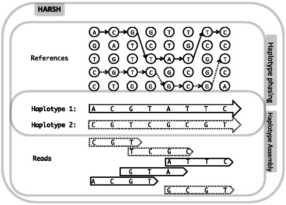
An illustration of haplotype inference problems. The two chromosomes for an individual are unknown to us at first. Sequencing technology produces a set of reads, each of which originates from one of the two chromosomes. We also have a set of reference haplotypes, which are from the same population as the donor. Haplotype assembly aims to assemble the two donor haplotypes by only using the read information. Haplotype phasing problem aims to phase the two haplotypes by mosaic copies from the reference haplotypes. However, our approach HARSH takes into account both read information and reference panel for more accurate haplotype inference

We can formalize this problem as follows. Suppose that we only consider L biallelic SNPs and M reads. Each read is represented by , where 0 stands for unobserved SNP in jth read, −1 and 1 stand for observed minor and major alleles, respectively. Because the homozygous site does not affect the haplotype phasing, we only consider heterozygous sites. Therefore, the objective is to find a sequence of haplotype and its complementary where , to minimize the total number of flipped loci within reads, such that every read can be perfectly assigned to one of the haplotypes. Another necessary variable for the model is the read origin indicator . If , the jth read is assumed to have been generated from haplotype h, and if , the jth read is from the complementary haplotype . We assume the read generation process is as follows. First, we randomly pick one of the haplotypes () with equal probability, and then sample the read starting position from one of the L possible positions in the genome. If we consider the read generation processing is error free, then we have . However, if the read generation process is error-prone and ε indicates the rate of sequencing error then with probability , we have , and with probability ε, we have . An illustrative example is given in Figure 2.

Fig. 2.

A graphical model for haplotype assembly. In this example, two reads and four heterozygous SNPs are considered. Read 1 covers the SNPs 1, 2 and 3. Read 2 covers SNPs 2, 3 and 4. The variables stands for the haplotype. The variable stands for whether the read is from haplotype h or the complementary

We can formalize the connection between the haplotypes and read origin variables into the following probabilistic distribution. For each possible values of the haplotypes and read origin variables, we can calculate its probability as follows:

(2)

where

and the variables , and are vectors and matrix composed of scalar variables r, h and x. The variable Z is a normalization constant to ensure . The functions θ and η specify edge potentials that favor h and r to be of equal values and opposite values, respectively. The model parameter μ controls the ‘heat’ of the probabilistic model. Generally speaking, the probability distribution is smoother when μ is small and sharper when μ is large.

Lemma 1 —

The maximum a posteriori (MAP) assignment of (2) corresponds to the MEC haplotype for any .

Proof —

We can prove by constructing the MEC haplotype from MAP assignment. Let and denote the MAP assignment of our probabilistic model, and the corresponding probability calculated from (2) will be

where n is the number of edges getting potential and m is the number of edges getting potential based on the configuration and . As for and the number of edges is fixed, this MAP assignment and is actually minimizing the number of edges getting potential . We can use this haplotype and flip every read bit corresponding to the edge getting potential . The resulting MEC score for will be m, which is minimized.

Suppose that there exists another haplotype with MEC score . It suggests that we can flip only read bit then all the reads will be perfectly assigned to one of the haplotypes. We keep those assignments into the variable . Thus, we should have

By definition, ; thus, , which contradicts the fact that and is the MAP assignment maximizing the configuration probability. By this contradiction, we can conclude that there does not exist and with MEC score .

2.3 Haplotype phasing with sequencing data and reference

Current haplotype assembly methods mainly focus on de novo assembly, which uses short reads as the only information source. This is partially owing to the complexity of extending the method to the scenario of assembly using reference. On the other hand, current haplotype phasing methods only use the reference panel and genotype likelihood in each SNP but ignore the multi-SNP information in the reads. We aim to use both the reference panel and sequencing data to perform haplotype phasing as shown in Figure 1. Formally, suppose that we are only considering L biallelic SNPs, M reads and N reference haplotypes. Each read is represented by , where 0 stands for unobserved SNP in jth read. The objective is to find two haplotypes, , where . We want to find the two haplotypes with small number of inconsistent loci with reads, as well as more consistent with reference haplotypes. We use another set of variables, , where , to stand for the assignment of each loci to reference haplotypes. We also need a set of variables , where stands for the haplotype that each read originates from. An illustrative example of the graph structure is given in Figure 3.

Fig. 3.

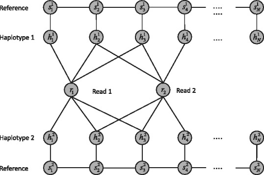
A graphical model for haplotype phasing with reference. The variables h¹ and h² stand for the first and second haplotypes. The variables specify whether the read comes from the first haplotype or second haplotype. The variable s¹ and s² specify which haplotype in the reference is generating the haplotype h¹ and h², respectively

Similar to the previous section, we can formalize the connection between the three variables H, R and S into the following probabilistic distribution. For each possible values of H, R and S, we can calculate its probability as follows:

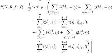(3)

where we have four edge potential functions. The functions θ and η are defined similarly as in (2) except that there would be no penalty if the read is assigned by r to the other haplotype.

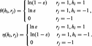The edge potential function ξ specifies the ‘haplotype copying’, which is motivated that the predicted haplotype is a mosaic of reference haplotypes with a small number of differences. In this case, the predicted haplotypes are similar to reference haplotype s¹ and s² at position i.

where G_ij stands for the jth allele in ith reference haplotype. Thus, stands for the ith allele in th reference haplotype. Moreover, we use the following function to model the transition probability in haplotype copying model (Li and Stephens, 2003).

where and r_i is the per generation genetic distance between site i and site i + 1, and N_e is a constant.

This probabilistic model provides us a disciplined way to infer the most probable haplotype given a set of reads and a set of reference haplotypes. It extends the haplotype copying model (Li and Stephens, 2003) from genotype input to sequencing data input. It also extends the haplotype assembly problem in previous section to a more general case where the reference panel can be used to improve the phasing. We are then able to design efficient sampling approach to find the most possible configurations of H, R and S that maximize the probability given in Equation (3).

2.4 Efficient sampling

Haplotype assembly without reference. The bipartite structure in Figure 2 suggests an efficient procedure for sampling. For fixed one layer of the bipartite graph, the variables in the other layer will be independent on each other. Thus, the conditional probability in Equation (1) of Gibbs sampler can be significantly reduced. Formally, following the standard procedure of Gibbs sampling, we can sample haplotype from the conditional probability for fixed read origins. The sampling ratio can be calculated as follows:

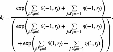(4)

Similarly, we can also do a similar Gibbs sampling step for read origin for fixed haplotype. The sampling ratio can be calculated as follows:

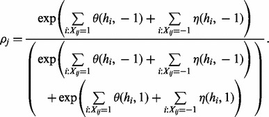(5)

The complete sampling algorithm for haplotype assembly is shown in Algorithm 1. As default, we use 10 000 rounds for sampling.

Haplotype phasing with reference. The sampling for haplotype phasing with both sequencing data and reference from the graph in Figure 3 is more challenging. However, we can still take advantages of the special structure of the graph and perform efficient sampling procedure. Following the idea of Gibbs sampler, we will alternatively (i) sample read origin R for fixed haplotype H and reference assignment S; (ii) sample S for fixed R and H; (iii) sample H for fixed R and S. The step (i) is similar with that in haplotype assembly. Formally, the sampling ratio for read origin can be calculated by

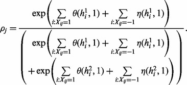(6)

Algorithm 1 Sampling Algorithm for Haplotype Assembly.

• 1: Randomly initialize haplotype H.
• 2: For fixed haplotype H, sample read origin R. For probability , we get , and for probability , we get , where the ratio ρ can be calculated as in (5).
• 3: For fixed read origin R, sample haplotype H. For probability , we get , and for probability , we get , where the ratio δ can be calculated as in (4).
• 4: Repeat steps 2 and 3 for sufficient rounds until equilibrium.
• 5: Collect samples by repeating steps 2 and 3, and output the one with highest probability.

The step (iii), sampling of haplotype H for fixed read origin R and reference assignment S is a straightforward extension from Equation (4). The modification is based on the extra edge between reference penal variables S and haplotype H. Formally, the sampling ratio for the first haplotype can be calculated by

(7)

where

The sampling ratio is similar with . Similarly, we can obtain the sampling ratio for the second haplotype as follows:

(8)

where

The step (ii), sampling for the haplotype reference panel variables S for fixed read origin R and haplotype H is challenging. The difficulty comes from the dependency between the variables s_i and , and the large number of possible values for each s_i. Note that unlike the binary variables h and r, the variable , where N is the number of reference haplotypes. Thus, straightforward Gibbs sampler would be inefficient in this case. To tackle this computational challenge, we resort to the following Markov chain sampling procedure (Liu, 2008). The joint distribution over all variables in S can be written as follows:

(9)

where

Sampling directly from is still tedious. However, we can convert the to multiplication series of probability functions as follows: . Then sampling from and sampling backward using those conditional probabilities becomes trivial. We can use dynamic programming to convert the distribution to the alternative form. We define

and

Thus, we can compute the normalization factor efficiently using dynamic programming, and then we can compute the marginal probability . Moreover, we can backward compute similarly. Note that a naive implementation of this step would result in a complexity of quadratic in the number of reference haplotypes. We take advantage of the symmetry in the haplotype coping model to reuse computation to achieve runtime linear in the number of reference haplotypes.

An outline of the sampling algorithm for haplotype phasing with sequencing data and a reference panel is given in Algorithm 2. As default, we use 10 000 rounds of sampling.

Algorithm 2 Sampling Algorithm for Haplotype Phasing.

• 1: Randomly initialize haplotype H
• 2: For fixed haplotype H, sample read origin R using sampling ratio in (6).
• 3: For fixed haplotype H sample haplotype reference S following Markov chain sampling procedure described after (9).
• 4: For fixed read origin R, and haplotype reference S, sample haplotype H using sampling ratio in (7).
• 5: Repeat steps 2, 3 and 4 for sufficient rounds until equilibrium.
• 6: Collect samples by repeating steps 2, 3 and 4. Output samples with highest probability.

3 EXPERIMENTAL RESULTS

3.1 Datasets and experimental settings

We performed simulation experiments using HapMap Phase II data (International HapMap Consortium, 2005) and 1000 Genomes data (Durbin, R. et al., 2010). For our simulations, we used the 60 parental individuals of CEU populations from HapMap Phase II as well as 60 individuals randomly chosen from the European populations for 1000 Genomes data. Although our method is scalable to the entire genome, for the purpose of demonstration, we use only chromosome 22 as representative of the rest of the genome, as it is the shortest chromosome. Because we are performing many simulations, we restrict our results to the 35 421 SNPs in chromosome 22 of the HapMap data, and the first 30 000 SNPs in chromosome 22 of 1000 Genomes data, which span ∼3 Mb. The datasets are publicly available at http://mathgen.stats.ox.ac.uk/impute/ and http://hapmap.ncbi.nlm.nih.gov/.

We evaluate our method using a leave-one-out procedure. In each round, we infer the haplotype for one individual using simulated sequencing data and the haplotypes of the other 59 individuals as reference panel. This procedure is repeated 60 times and all the evaluation metrics are averaged. The reads are simulated uniformly across chromosome 22 for a given coverage. The read length in each end of a pair-end read is fixed but the gap between the two ends follow a normal distribution with fixed mean and standard deviation. Errors are inserted in the read at a rate ε.

We evaluate our method HARSH using the standard metric for genotyping and phasing accuracy: genotyping error rate and switching error rate. The genotyping error rate is the proportion of wrongly predicted genotypes, and the switching error is the proportion of switches in the inferred haplotypes to recover the correct phase in an individual. The total error rate is the sum of genotyping error rate and switching error rate. We also use percentage improvement when comparing two methods. The percentage improvement is computed as the error rate difference between two methods normalized by the error rate of baseline method. For example, suppose that HARSH has error rate x and baseline method has error rate y, the improvement of HARSH over the baseline method would be .

We fixed the parameters , and for all our experiments. From our experience, the performance of the proposed method is not sensitive to parameter tuning. Using μ from 1 to 10 and ω from 0.001 to 0.005 does not affect the performance significantly. The sequencing error is standard sequencing error rate.

All experiments are performed in a cluster machine where each node has 8–16 cores 3.0 GHz CPU and 1–16 GB memory. Jobs are submitted in a parallel manner but each job uses only one node.

3.2 HapMap simulations

We use HapMap dataset to evaluate our method HARSH. We compare our method with three other state-of-the-art methods: the HMM at the core of the IMPUTE method (Howie et al., 2009), BEAGLE (Browning and Browning, 2009) and Hap-SeqX (He and Eskin, 2013). Because IMPUTE does not support haplotype phasing for uncovered SNPs, for a fair comparison, we re-implemented the basic HMM model of the IMPUTE v1.0, which uses the pre-defined genetic map information for transition probability. We will refer to our implementation of the HMM model in IMPUTE method as IMPUTE*. In our modified version, we use the read count for each SNP as input to IMPUTE* method. The likelihood of read count from genotype is used as the emission probability for the HMM model. Then the Viterbi algorithm is used to decode two paths from the reference panel, which are most likely to generate the read counts in each SNP. The two paths in reference panel also give the two predicted haplotypes. Because the latest implementation of IMPUTE (Howie et al., 2009) is not able to phase, we also compared our approach with BEAGLE 3.3.2 (Browning and Browning, 2009), a widely used approach for haplotype phasing and imputation.

We first use the HapMap dataset to show that haplotype assembly without a reference panel will underperform haplotype phasing with a reference panel. The main reason is that there are not enough long reads covering all continuous heterozygous SNPs. Thus, haplotype assembly cannot do more than random guess between two continuous heterozygous SNPs if there is no read spanning them. We can compute a lower bound of the number of switches for haplotype assembly as where K is the number of those gaps, assuming the MEC score to be zero. For pair-end reads with fixed length 1000 bp mean and 100 bp standard deviation, we evaluate our method using six levels of sequencing coverages: 1×, 2×, 4×, 6×, 8× and 10×. As shown in Figure 4a, higher coverage does not help haplotype assembly to achieve similar performance than haplotype phasing methods. At fixed coverage 4×, we simulated pair-end reads with 1000, 2000, 3000 and 4000 bp in each end. As shown in Figure 4b, we can observe that the lower bound of haplotype assembly achieves similar performance as haplotype phasing only under the unrealistic read length 4000 bp. Also, at 4× coverage, we can observe that our method can improve ∼44% over BEAGLE and ∼37% over IMPUTE in terms of numbers of switches.

Fig. 4.

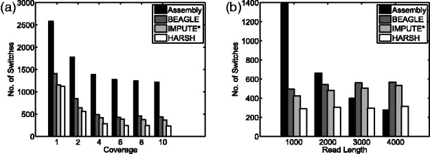
The number of switches within heterozygous SNPs for haplotype assembly, BEAGLE, IMPUTE* and HARSH. The number of switches of haplotype assembly is estimated by the lowest bound. (a) Varying coverage for fixed read length 1000 bp. (b) Varying read length for fixed coverage 4X

For simulated pair-end reads with 1000 bp for each end at 1× coverage, only 32% reads contain one SNP and ∼26% of the reads contain more than three SNPs. On average, every read contains around 2.8 SNPs. Following the procedure similar to that of He and Eskin (2013), we divide the chromosome into overlapping chunks containing 1200 SNPs each and run our method on each chunk independently. The final haplotypes are then constructed by stitching together the haplotypes from each chunk. Chromosome 22 is divided into 36 chunks. The total error rate for both IMPUTE* and HARSH are shown in Figure 5. We can observe from the figure that HARSH consistently performs better than IMPUTE* across all 36 chunks. The average improvement over IMPUTE* is 7.6%. We then concatenated those haplotype chunks by minimizing the mismatches in the overlap region between two adjacent chunks. After concatenation, the overall error rate for HARSH is 4.01% for chromosome 22, compared with 4.42% for IMPUTE*. The overall improvement is 9.3% over IMPUTE*.

Fig. 5.

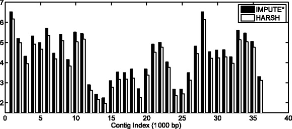
The error rate for IMPUTE* and our method for each chunk of length 1200 SNPs in chromosome 22. The error rate consists of both genotyping error for all SNPs and switch error within heterozygous SNPs

We compare HARSH with a previous method for combining multi-SNP reads with a reference panel, Hap-SeqX (He and Eskin, 2013). Hap-SeqX is an approximation to the dynamic programming approach of the Hap-Seq method (He et al., 2012), which optimizes a similar objective function to HARSH. Hap-SeqX only searches a fraction of the search space compared with Hap-Seq by only storing the top values at each state. However, Hap-SeqX is still an expensive method in both time and memory usage. In this experiment, we use the default parameters of Hap-SeqX, where specifies that the algorithm saves the top 1% of values for each state. On addition, Hap-Seq and Hap-SeqX, unlike HARSH, can only handle up to three SNPs in a read and split reads containing more SNPs into multiple reads. The performance comparisons are shown in Table 1. HARSH and IMPUTE* have similar running time. HARSH takes ∼10 min compared with IMPUTE* 5 min on chromosome 22. Both these methods compare favorably with Hap-SeqX, which takes 5 h for the same dataset. Cross validation of 60 individuals would be prohibitive for Hap-SeqX. Thus, we compare all these three methods using only the first individual in HapMap dataset. The results averaged more than 36 chunks. We can see that Hap-SeqX improves by ∼12.53% from the baseline method IMPUTE*, and HARSH significantly improves by 21.34% from IMPUTE*. We conducted significance test (paired-sample t-test) on the improvement of HARSH over Hap-SeqX and IMPUTE*. The test results show that HARSH significantly outperforms both Hap-SeqX and IMPUTE* with P and P, respectively. Overall, the comparison shows that HARSH is the most accurate and practical method among existing methods.

Table 1.

Comparison between IMPUTE*, Hap-SeqX and HARSH on a HapMap dataset with 1 donor individual, 59 reference individuals and 35 421 SNPs

Methods	Error rate (switch, genotyping)	Time
IMPUTE*	0.04836 (0.00804, 0.04033)	∼5 min
Hap-SeqX	0.04230 (0.00726, 0.03504)	∼5 h
HARSH	0.03804 (0.00664, 0.03140)	∼10 min

Note: Read length of 1000 bp and 1× coverage are simulated.

To fully evaluate the performance of our method, we apply our method to cases with different coverages and read lengths. For pair-end reads with fixed length 1000 bp mean and 100 bp standard deviation, we evaluate our method using six levels of sequencing coverages: 1×, 2×, 4×, 6×, 8× and 10×. The result is shown in Figure 6a. As expected, the performance improvement of HARSH over BEAGLE and IMPUTE* becomes more significant when the coverage increases. The reason we expect this is that the higher the coverage, the larger number of reads that span multiple SNPs. HARSH is able to take advantage of the multi-SNP information within those reads but BEAGLE and IMPUTE* can not take advantage of that. In Table 2, we show the genotyping and switching error rate of HARSH and IMPUTE* method for different coverages. It can be observed that both genotyping error and switching error are significantly reduced by HARSH over BEAGLE and IMPUTE*. It is also worth mentioning that 4× seems to be the best choice in terms of the compromise between the cost of coverage and achieved accuracy. The coverage 4× gives 0.28% genotyping error and 0.62% switching error. However, the improvement of higher coverage than 4× is limited.

Fig. 6.

Performance of BEAGLE, IMPUTE* and HARSH for varying coverage and read length on HapMap. (a) Varying coverage for fixed read length 1000 bp. (b) Varying read length for fixed coverage 4X

Table 2.

Genotyping and switching errors (%) for varying coverages on HapMap dataset

Coverage	1×	2×	4×	6×	8×	10×
Genotyping Error
BEAGLE	4.21	1.94	0.59	0.22	0.10	0.04
IMPUTE*	3.59	1.53	0.56	0.30	0.17	0.12
HARSH	3.42	1.28	0.28	0.08	0.04	0.02
Switching Error
BEAGLE	0.97	1.04	1.05	1.11	1.23	1.23
IMPUTE*	0.82	0.87	0.90	0.94	0.97	0.98
HARSH	0.72	0.67	0.62	0.63	0.65	0.65

Note: Read length is fixed to be 1000 bp.

We also evaluate HARSH with different read lengths. At fixed coverage 4×, we simulated pair-end reads with 1000, 2000, 3000 and 4000 bp in each end. The results are shown in Figure 6b. It is not immediately intuitive why the genotyping error rates for BEAGLE, IMPUTE* and HARSH increase when the read length increases. A possible reason is that longer reads for a fixed coverage result in fewer total reads and larger gaps without any coverage. In other words, longer reads result in less random read bits across the chromosome. An extreme example is that the gap will be half of the genome on average if the read length is equal to the genome size and coverage is 1×. Sequentially, larger gap where no reads cover will potentially harm the imputation and haplotype phasing accuracy. However, we can still see that the performance gap between BEAGLE or IMPUTE* and HARSH is enlarged while the read length increases. This is attributed to the ability of HARSH to leverage the multi-SNP information in longer reads. In Table 3, we show the improvement of HARSH over BEAGLE and IMPUTE*. The improvement is basically from the reduced switching error, which is reduced from 0.62 to 0.48% by HARSH but not by IMPUTE*. The genotyping error for both methods increases at the same pace because of the larger gaps caused by longer reads. The error rates for BEAGLE, IMPUTE* and HARSH increase from 0.59 to 0.79%, from 0.56 to 0.85% and from 0.28 to 0.48%, respectively, when the read length increases from 1000 to 4000 bp. But HARSH consistently performs better than BEAGLE and IMPUTE even while the genotyping error rate is increasing.

Table 3.

Genotyping and switching errors (%) for varying read lengths on HapMap dataset

Read length	1000 bp	2000 bp	3000 bp	4000 bp
Genotyping error
BEAGLE	0.59	0.67	0.74	0.79
IMPUTE*	0.56	0.70	0.77	0.85
HARSH	0.28	0.37	0.40	0.48
Switching error
BEAGLE	1.05	1.10	1.07	1.07
IMPUTE*	0.90	0.93	0.94	0.94
HARSH	0.62	0.57	0.49	0.48

Note: Coverage is fixed to be 4×.

3.3 1000 Genomes simulations

The 1000 Genomes project is an ongoing project that uses HTS technology to collect the genetic variant data across many individuals with the goal of characterizing rare variants, which are not present in HapMap. This provides us the opportunity to evaluate our method using simulations that will realistically capture the distributions of rare variants and more accurately reflect a tubal performance. We simulate realistic paired end reads, which have 100 bp for each end, and a gap size following a normal distribution with 100 bp mean and standard deviation of 10 bp. Only 22% reads contain only one SNP and ∼55% reads contain more than three SNPs. On average, every read covers around 3.1 SNPs. Following the same settings as what we did for HapMap data, we test HARSH for different coverages and read lengths. The results for coverage 1×, 2×, 4×, 8×, 16× and 32× are shown in Figure 7a. We observe that the error rate does not further drop after coverage 8×. At coverage 8×, the improvement of HARSH over IMPUTE* is 29% from 0.021 to 0.015 in terms of error rate. Thus, for fixed coverage 8×, we simulate pair-end reads with 100, 200, 300 and 400 bp in each end. The results are shown in Figure 7b. We observe that, HARSH, unlike IMPUTE*, benefits from using longer reads, as it contains more multi-SNP reads than shorter reads. Thus, as expected, the performance gap between IMPUTE* and HARSH increases as the read length increases. However, in Figure 7b, we do not see that the error rate increases when the read length increases as in Figure 6b. A possible reason is that the SNPs are much denser in 1000 Genomes data than HapMap data, and we simulated much shorter reads for 1000 Genomes data. Thus, the gap caused by 400 bp read length would be much shorter than previous 4000 bp read length for HapMap dataset. The reference haplotype panel could well take advantage of Linkage Disequilibrium effect to recover those gaps. Therefore, the error rate for IMPUTE* keeps almost the same for different read lengths but our method HARSH reduces the error rate by incorporating more multi-SNP read information when the read length increases.

Fig. 7.

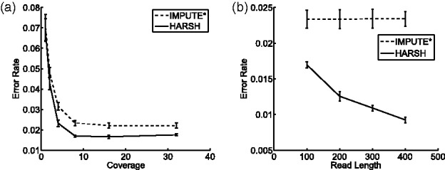
Performance of IMPUTE* and HARSH for varying coverage and read length on 1000 genomes. (a) Varying coverage for fixed read length 1000 bp. (b) Varying read length for fixed coverage 4X

4 CONCLUSION AND DISCUSSIONS

Haplotype phasing plays an important role in a wide variety of genetic applications. Although it is possible to determine haplotypes using laboratory-based experimental techniques, these approaches are expensive and time-consuming. Recently, Kitzman et al. (2011) were able to generate the complete phased sequence of a Gujarati individual using a Fosmid library. Unfortunately, this method is not easily scalable to phasing more than one individual. Thus, the need for a practical computational method for haplotype phasing remains.

We have presented HARSH, an efficient method that combines multi-SNP read information with reference panels of haplotypes for improved genotype and haplotype inference in sequencing data. Unlike previous phasing methods that use read counts at each SNP as input, our method takes into account the information from reads spanning multiple SNPs. HARSH is able to efficiently find the likely haplotypes in terms of the marginal probability over the genotype data. Using simulations from HapMap and 1000 Genomes data, we show that our method achieves superior accuracy than existing approaches with decreased computational requirements. In addition, we evaluate our method as function of coverage and read length, showing that our method continues to improve as read length and coverage increases.

Funding: National Science Foundation (0513612, 0731455, 0729049, 0916676, 1065276 and 1320589 to W.Y., F.H., Z,W. and E.E.); National Institutes of Health (K25-HL080079, U01-DA024417, P01-HL30568 and PO1-HL28481 to W.Y., F.H., Z,W. and E.E.; R03-CA162200 and R01-GM053275 to B.P.).

Conflict of Interest: none declared.

REFERENCES

- Aguiar D, Istrail S. HapCompass: a fast cycle basis algorithm for accurate haplotype assembly of sequence data. J. Comput. Biol. 2012;19:577–590. doi: 10.1089/cmb.2012.0084. [DOI] [PMC free article] [PubMed] [Google Scholar]
- Bansal V, Bafna V. HapCUT: an efficient and accurate algorithm for the haplotype assembly problem. Bioinformatics. 2008;24:i153–i159. doi: 10.1093/bioinformatics/btn298. [DOI] [PubMed] [Google Scholar]
- Bansal V, et al. An MCMC algorithm for haplotype assembly from whole-genome sequence data. Genome Res. 2008;18:1336–1346. doi: 10.1101/gr.077065.108. [DOI] [PMC free article] [PubMed] [Google Scholar]
- Browning BL, Browning SR. A unified approach to genotype imputation and haplotype-phase inference for large data sets of trios and unrelated individuals. Am. J. Hum. Genet. 2009;84:210–223. doi: 10.1016/j.ajhg.2009.01.005. [DOI] [PMC free article] [PubMed] [Google Scholar]
- Duitama J, et al. Proceedings of the First ACM International Conference on Bioinformatics and Computational Biology. New York, NY: ACM; 2010. Refhap: a reliable and fast algorithm for single individual haplotyping; pp. 160–169. [Google Scholar]
- Duitama J, et al. Fosmid-based whole genome haplotyping of a hapmap trio child: evaluation of single individual haplotyping techniques. Nucleic Acids Res. 2012;40:2041–2053. doi: 10.1093/nar/gkr1042. [DOI] [PMC free article] [PubMed] [Google Scholar]
- Durbin R, et al. A map of human genome variation from population-scale sequencing. Nature. 2010;467:1061–1073. doi: 10.1038/nature09534. [DOI] [PMC free article] [PubMed] [Google Scholar]
- Fearnhead P, Donnelly P. Estimating recombination rates from population genetic data. Genetics. 2001;159:1299–1318. doi: 10.1093/genetics/159.3.1299. [DOI] [PMC free article] [PubMed] [Google Scholar]
- Geman S, Geman D. Stochastic relaxation, gibbs distributions, and the bayesian restoration of images. IEEE Trans. Pattern Anal. Mach. Intell. 1984;6:721–741. doi: 10.1109/tpami.1984.4767596. [DOI] [PubMed] [Google Scholar]
- He D, Eskin E. Hap-seqX: expedite algorithm for haplotype phasing with imputation using sequence data. Gene. 2013;518:2–6. doi: 10.1016/j.gene.2012.11.093. [DOI] [PubMed] [Google Scholar]
- He D, et al. Optimal algorithms for haplotype assembly from whole-genome sequence data. Bioinformatics. 2010;26:i183–i190. doi: 10.1093/bioinformatics/btq215. [DOI] [PMC free article] [PubMed] [Google Scholar]
- He D, et al. Proceedings of the 16th Annual International Conference on Research in Computational Molecular Biology (RECOMB) New York, NY: Springer; 2012. Hap-seq: an optimal algorithm for haplotype phasing with imputation using sequencing data; pp. 64–78. [DOI] [PMC free article] [PubMed] [Google Scholar]
- Howie B, et al. Genotype imputation with thousands of genomes. G3 (Bethesda) 2011;1:457–470. doi: 10.1534/g3.111.001198. [DOI] [PMC free article] [PubMed] [Google Scholar]
- Howie BN, et al. A flexible and accurate genotype imputation method for the next generation of genome-wide association studies. PLoS Genet. 2009;5:e1000529. doi: 10.1371/journal.pgen.1000529. [DOI] [PMC free article] [PubMed] [Google Scholar]
- Hugot JP, et al. Association of nod2 leucine-rich repeat variants with susceptibility to crohn’s disease. Nature. 2001;411:599–603. doi: 10.1038/35079107. [DOI] [PubMed] [Google Scholar]
- International HapMap Consortium. A haplotype map of the human genome. Nature. 2005;437:1299–1320. doi: 10.1038/nature04226. [DOI] [PMC free article] [PubMed] [Google Scholar]
- Kang HM, et al. EMINIM: an adaptive and memory-efficient algorithm for genotype imputation. J. Comput. Biol. 2010;17:547–560. doi: 10.1089/cmb.2009.0199. [DOI] [PMC free article] [PubMed] [Google Scholar]
- Kitzman JO, et al. Haplotype-resolved genome sequencing of a gujarati indian individual. Nat. Biotechnol. 2011;29:59–63. doi: 10.1038/nbt.1740. [DOI] [PMC free article] [PubMed] [Google Scholar]
- Lazzeroni LC. A chronology of fine-scale gene mapping by linkage disequilibrium. Stat. Methods Med. Res. 2001;10:57–76. doi: 10.1177/096228020101000104. [DOI] [PubMed] [Google Scholar]
- Li N, Stephens M. Modeling linkage disequilibrium and identifying recombination hotspots using single-nucleotide polymorphism data. Genetics. 2003;165:2213–2233. doi: 10.1093/genetics/165.4.2213. [DOI] [PMC free article] [PubMed] [Google Scholar]
- Li Y, et al. MaCH: using sequence and genotype data to estimate haplotypes and unobserved genotypes. Genet. Epidemiol. 2010;34:816–834. doi: 10.1002/gepi.20533. [DOI] [PMC free article] [PubMed] [Google Scholar]
- Liu JS. Monte Carlo Strategies in Scientific Computing. New York, NY: Springer; 2008. [Google Scholar]
- Long Q, et al. HI: haplotype improver using paired-end short reads. Bioinformatics. 2009;25:2436–2437. doi: 10.1093/bioinformatics/btp412. [DOI] [PMC free article] [PubMed] [Google Scholar]
- Myers SR, Griffiths RC. Bounds on the minimum number of recombination events in a sample history. Genetics. 2003;163:375–394. doi: 10.1093/genetics/163.1.375. [DOI] [PMC free article] [PubMed] [Google Scholar]
- Pasaniuc B, et al. Extremely low-coverage sequencing and imputation increases power for genome-wide association studies. Nat. Genet. 2012;44:631–635. doi: 10.1038/ng.2283. [DOI] [PMC free article] [PubMed] [Google Scholar]
- Rioux JD, et al. Genetic variation in the 5q31 cytokine gene cluster confers susceptibility to Crohn disease. Nat. Genet. 2001;29:223–228. doi: 10.1038/ng1001-223. [DOI] [PubMed] [Google Scholar]
- Sabeti PC, et al. Detecting recent positive selection in the human genome from haplotype structure. Nature. 2002;419:832–837. doi: 10.1038/nature01140. [DOI] [PubMed] [Google Scholar]
- Xie M, et al. A fast and accurate algorithm for single individual haplotyping. BMC Syst. Biol. 2012;6(Suppl 2):S8. doi: 10.1186/1752-0509-6-S2-S8. [DOI] [PMC free article] [PubMed] [Google Scholar]