Non-rigid Registration of Longitudinal Brain Tumor Treatment MRI

Abstract

To evaluate changes in brain structure or function, longitudinal images of brain tumor patients must be non-rigidly registered to account for tissue deformation due to tumor growth or treatment. Most standard non-rigid registration methods will fail to align these images due to the changing feature correspondences between treatment time points and the large deformations near the tumor site. Here we present a registration method which jointly estimates a label map for correspondences to account for the substantial changes that may occur during tumor treatment. Under a Bayesian parameter estimation framework, we employ different probability distributions depending on the correspondence labels. We incorporate models for image similarity, an image intensity prior, label map smoothing, and a transformation prior that encourages deformation near the estimated tumor location. Our proposed algorithm increases registration accuracy compared to a traditional voxel-based registration method as shown using both synthetic and real patient images.

I. Introduction

Over the course of brain tumor treatment, resection, radiation therapy, and chemotherapy require that the patient be imaged at several time points to both prepare for and follow the progress of treatment. These longitudinal images also allow for the study of structural and functional changes that may occur as the disease or therapy progresses. To properly evaluate these changes, the longitudinal set of brain images must first be aligned. The tissue deformation that may occur over time due to lesion growth, tumor removal, or successful treatment requires a non-rigid registration method be used.

As described below, while some techniques have been proposed to deal with unmatched features, the popular and traditional non-rigid registration methods (e.g., [1], [2], [3]) assume that all features are present in both images to be registered. However, this one-to-one correspondence assumption will likely be violated in the case of longitudinal brain tumor data due to the effects of treatment. For example, successful radiation or chemotherapy may shrink the tumors and reduce cerebral edema, producing a change in intensity correspondence. Tumor resection will result in missing tissue correspondences and may also cause signal changes due to trauma or formation of scar tissue. A traditional voxel-based registration method will attempt to match the areas with missing or changed correspondences and will likely cause misalignment of actual corresponding structures near the lesion, which is often the region we are most interested in matching.

A brief review of recent methods which address substantially changed data due to tumor growth or brain resection is outlined here. An algorithm for aligning pre- and intra-operative tumor resection images was presented in [4] which required first extracting points from the images to be matched. For registration of brain tumor images with a normal atlas, biomechanical models have been used to simulate tumor growth and mass effect in the normal brain before registering to the patient image [5]. A demons-based method to handle resection and retraction in the intraoperative brain was introduced and tested on limited 2D data in [6]. One approach targeted at the general problem of partial data was proposed by [7]. However, their estimation for missing data was based only on the given images. For our data, we know how the intensities of the tumor and resection may appear a priori and expect large deformations closer to the lesion; we thus aim to include this information to facilitate the registration process.

In initial efforts related to the current work, we registered pre-operative images to a single post-resection time point [8]. We now propose a complete, robust strategy especially tailored to align pre-treatment brain tumor images to any one of a number of time points over a longitudinal dataset. The key to our approach is the inclusion of a label map to indicate matching vs. missing correspondences. Given the labels, we use a different probability distribution to describe what we expect under each condition. This label map is simultaneously estimated with the registration and other model parameters under a maximum a posteriori (MAP) framework using a technique inspired by [9]. A Bayesian approach allows us to include prior models for the image intensities expected in T1-gadolinum enhanced MRI, the registration parameters to encourage deformation near the tumor region, and the estimation of a smooth label map.

II. Methods

A. Registration Framework

Our aim is to align a target image T at time point t > 1 to a source image S at time point 1 by finding the best registration parameters R̂ which map voxel x in S to voxel R̂(x) in T. Let L be a label map corresponding to S to segment the different correspondence regions. For brain tumor images, we will use 6 labels to represent the background, voxels with matching correspondence, resection, active tumor, necrotic tumor, and edema. In a marginalized MAP framework,

$$\widehat{R}=\underset{R}{arg\; max\; log}\sum _{L}p(R,L|S,T).$$ (1)

To solve the problem, we employ a variant of the expectation-maximization (EM) algorithm, which iterates between updating the label map given the current transformation in the E-step and updating the registration parameters given the current label map probabilities in the M-step. Specifically, in the M-step,

$$R^{k+1}=\underset{R}{argmax}{E}_{L|S,T,R^k}logp(R,L|S,T),$$ (2)

where R^k is the estimate for the registration parameters from iteration k. Assuming the intensities in S only depend on the label map, we simplify (2) as

$$R^{k+1}=\underset{R}{argmax}(E_{L|S,T,R^k}logp(T|S,R,L)+E_{L|S,T,R^k}logp(R|L)).$$ (3)

We assume independence and write the first expectation as a sum over all voxels in S and possible labels in L. For the second term, we would like to model the registration parameters as depending on the entire map. Since calculating the expectation over all possible maps is intractable, we apply a classification EM approach [10] and consider only the most likely label map from the current iteration L^k+1. The registration update becomes

$$R^{k+1}=\underset{R}{argmax}(\sum _{\text{x}\in S}\sum _{l\in L}p(L(\text{x})=l|S,T,R^k)\cdot logp(T(R(\text{x}))|S,R,l)+\sum _{\text{x}\in S}logp(R(\text{x})|L^{k+1})).$$ (4)

Since we are no longer maximizing a strict expectation of the posterior, the method becomes a generalized EM (GEM) algorithm. GEM is still guaranteed to converge to a local maximum and it greatly simplifies computation.

The E-step computes the probability of label map assignments given the registration parameters from the M-step. Using Bayes' rule and assuming a change in L (x) will produce only a small change in p (R (x) | L^k+1), we have

$$p(L(\text{x})=l|S,T,R^k)=\frac{p(T(R^k(\text{x}))|S,R^k,l)p(S(\text{x})|l)p(l)}{\sum _{l^{\prime }}p(T(R^k(\text{x}))|S,R^k,l^{\prime })p(S(\text{x})|l^{\prime })p(l^{\prime })}.$$ (5)

We estimate the final label map as $\widehat{L}(\text{x})=\underset{l}{argmax}p(L(\text{x})=l|S,T,\widehat{R})$.

B. Implemented Probability Models

This section describes a specific implementation of the probability distributions and models to calculate (4) and (5).

Similarity Measure

The likelihood model p (T (R (x)) | S, R, L(x) = l) acts like the similarity measure in a traditional registration method. Since we are registering images of the same type, we assume corresponding voxels should match intensities and use (S (x), σ_t). Given a background voxel, we again use a normal distribution (S (x), σ_b) but assign σ_b > σ_t since we are not interested in aligning background. Voxels assigned to an abnormal class, i.e. resection, active tumor, necrosis, or edema, are assumed to be missing correspondences in T, leading us to choose a uniform distribution $\frac{1}{\mathit{\text{C}}}$ to allow them to match any intensity. We automatically estimate the matching tissue standard deviation σ_t using a conditional maximization approach in the M-step [11]:

$${\sigma }_t^{k+1}=\sqrt{\frac{\sum _{\text{x}\in S}p(L(\text{x})=l|S,T,R^k){(T(R^k(\text{x}))-S(\text{x}))}^2}{\sum _{\text{x}\in S}p(L(\text{x})=l|S,T,R^k)}}.$$ (6)

In the beginning of the GEM algorithm, σ_t will have a larger value, allowing for a broader capture range for misaligned voxels. As the images become more aligned in later iterations, σ_t will decrease, encouraging further finer alignment. In addition, we update the uniform distribution parameter C^k+1 such that voxels that have intensity differences S (x) − T (R(x)) further than 2 standard deviations ${\sigma }_t^{k+1}$ away from a 0-mean Gaussian are considered more likely to belong to one of the abnormal classes.

Intensity Prior Given the Label Map

For the source image intensity prior p (S (x) | L (x) = l), we assume the MRI signal is characterized by the abnormal tissues. We model background voxels as following a normal distribution with 0 mean and small standard deviation. For the resection, active tumor, necrosis, and edema, we model the intensity of each class as following a normal distribution with mean and standard deviation estimated from a training set of T1-weighted post-gadolinium brain tumor images. Voxels with valid correspondences are assumed to be of any intensity, and thus a uniform distribution is used.

Transformation Prior Given the Label Map

We use free-form deformations (FFDs) based on uniform cubic B-splines for the transformation model. For the prior p (R(x) | L), we wish to encourage larger deformations nearer the tumor region, while we expect the transformation to be more rigid farther away. Thus, we model p (R (x) | L) using a normal distribution with mean equal to the position of voxel x. Assuming independent motion along each coordinate, we assign a uniform standard deviation σ_x for each component. We set the variance to be inversely proportional to the distance d between voxel x and lesions in L,

$${\sigma }_{\text{x}}^2=\{\begin{array}{cc}{\sigma }_{\mathit{\text{min}}}^2+\frac{d_{\mathit{\text{tol}}}-d}{d_{\mathit{\text{tol}}}}({\sigma }_{\mathit{\text{max}}}^2-{\sigma }_{\mathit{\text{min}}}^2)& ,d\le d_{\mathit{\text{tol}}}\\ {\sigma }_{\mathit{\text{min}}}^2& ,d>d_{\mathit{\text{tol}}}\end{array},$$ (7)

where ${\mathit{\sigma }}_{\mathit{\text{min}}}^2$ and ${\mathit{\sigma }}_{\mathit{\text{max}}}^2$ are the minimum and maximum allowed variances and d_tol is the distance from the lesion beyond which we keep the variance constant. Here we set d_tol to be twice the B-spline control point spacing. The variances are updated in the M-step in iteration k using label map L^k.

Label Map Prior

We impose a Markov random field onto the label map. We can then write p (L) using a Gibbs distribution, $p(L)=\frac{1}{Z}\mathit{\text{exp}}[-\beta \sum _c{V}_c(L)]$, where Z is a normalizing constant and V_c (L) is the potential for clique c. Using a mean field-like approximation [12] and a Potts smoothing model, we have

$$p(L(\text{x})=l)=\frac{1}{Z_{\text{x}}^{\prime }(\beta )}\mathit{\text{exp}}[\beta \sum _{\text{n}\in N(\text{x})}\delta (l,L^k(\text{n}))],$$ (8)

where N (x) are the neighbors of x and we approximate the mean field using $L^k(\text{n})=\underset{l}{argmax}p(L(\text{x})=l|S,T,R^{k-1})$. We iteratively estimate the weighting parameter β conditional on the current registration parameters:

$${\beta }^{k+1}=\underset{\beta }{argmax}\sum _{\text{x}\in S}\sum _{l\in L}p(L(\text{x})=l|S,T,R^k)\cdot [logp(L(\text{x})=l|\beta )+logp(\beta )].$$ (9)

We assign a normal distribution on β with small mean and variance so that the indicator map estimation does not rely too strongly on the prior.

III. Results

We tested our joint registration and label map estimation (RALE) approach against a standard non-rigid registration (SNRR) method based on [1], implemented in BioImage Suite (BIS) [13]. Both techniques are based on direct intensity comparisons and use the same transformation model (B-spline based FFD) for a fair comparison.

A. Synthetic Examples

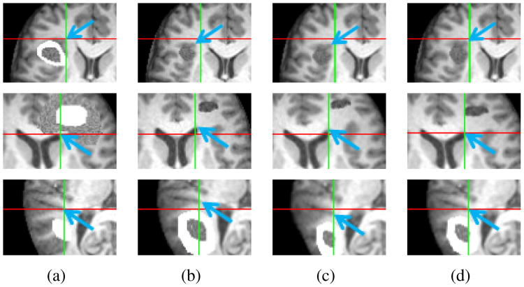
Synthetic longitudinal brain tumor images were created by selecting a slice from a normal brain and warping the image using a known transformation. A lesion was created in closely corresponding locations within a series. Three cases were created: 1) an active tumor with necrosis shrinks and shows no activity; 2) a large tumor with surrounding edema is resected; 3) a small active tumor grows. While the synthetic images may not simulate actual deformation seen with tumor growth or removal, the main problems of intensity and physical correspondence changes are highlighted and we have access to a ground truth displacement field for analysis.

Results are highlighted in Fig. 1, with each row corresponding to each series. Portions from the images at time points 1 and 2 are shown in Fig. 1(a) and 1(b), respectively. Images in Fig. 1(c) and 1(d) are the follow-up scans registered using SNRR and RALE, respectively. Blue arrows point to the same feature, while crosshairs mark the same physical location across a row. As seen with these markers, RALE aligns several prominent features better than SNRR.

Figure 1.

Results for synthetic brain tumor image sequences. (a) Time point 1. (b) Time point 2. (c) Time point 2 registered to time point 1 using SNRR. (c) Results using RALE. Crosshairs mark same location in the images in each row. Blue arrows highlight improved alignment of features in (a) with (d) compared to (c).

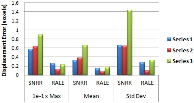
We calculated the maximum, mean, and standard deviation of displacement errors for pixels which had a corresponding match. As seen in Fig. 2, RALE greatly increased registration accuracy compared to SNRR. Paired one-tailed t-tests showed RALE significantly reduced each error measure (p < 0.05).

Figure 2.

Displacement errors for synthetic data registration results.

B. Patient Examples

We had available 2 sets of 3D patient data, each with 4 longitudinal images. Patient 1 had gamma knife treatment and a right frontal lesion resection at the last scan. Patient 2 underwent removal of a large lesion in the right parietal lobe, with the first scan taken prior to resection. The T1-weighted MRI were first skull-stripped, resampled to 1 mm voxel resolution, normalized such that intensity profiles were similar, and affinely aligned in BIS. Intensity prior parameters were estimated using all images except the pair to be registered.

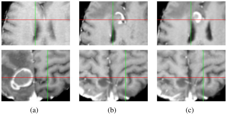
Each scan from a later time point was individually registered to the first scan, resulting in 3 test pairs for each patient. Figure 3 shows sample results from a pair of scans for patient 1 and 2. We see better alignment of various structures in the RALE results in Fig. 3(c) compared to SNRR in Fig. 3(b).

Figure 3.

Example results for patient 1 (first row) and patient 2 (second row). (a) Close up at time point 1. (b) SNRR results. (c) RALE results.

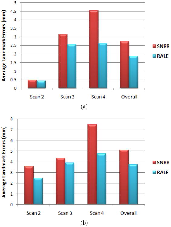
We measured landmark errors for 7 locations highly affected by the lesions in each patient (results far from lesions were similar for both methods and are not reported). Average errors for each image pair are shown in Fig. 4. While all errors increased with longer time between scans, RALE errors were lower and grew more slowly, suggesting RALE is more robust to large correspondence changes. Overall, SNRR and RALE resulted in average errors of 3.91 mm and 2.79 mm, respectively. Paired one-tailed t-tests showed that RALE significantly increased accuracy (p < 2e-6).

Figure 4.

Average landmark errors after registering (a) patient 1 and (b) patient 2 data.

Finally, we computed the dice coefficient to measure the overlap between true and estimated matching correspondence regions. The average dice coefficient for the 6 image pairs was 0.94.

IV. Discussion

In this work we presented a method for aligning longitudinal brain tumor treatment images. We simultaneously estimated a label map segmenting the different correspondence regions. We implemented a general expectation-conditional maximization algorithm and included an image similarity term, an intensity prior, a transformation prior, and a smooth label map prior. Results on synthetic and patient data demonstrated the improved accuracy of our proposed approach over a traditional non-rigid registration method.

While our method is reasonably accurate at detecting matching correspondences, it has more difficulty distinguishing between abnormal regions. One issue is that necrosis, edema and resection may produce very similar intensities. For the purpose of aligning matching features, this mislabeling is not so problematic since we use the same probability distribution for all types of missing correspondences in the similarity term. To better identify abnormal labels, we may include prior spatial information.

In the future, the proposed registration approach may be applied to clinical research studying changes in normal tissue or function of the brain following intervention. For example, by registering the serial images, the tissue movement could be tracked temporally to investigate factors that may determine the time it takes for tissue to deform into the resected region and the final size of the resection cavity.

References

- 1.Rueckert D, Sonoda LI, Hayes C, Hill DL, Leach MO, Hawkes DJ. Nonrigid registration using free-form deformations: application to breast mr images. IEEE T Med Imaging. 1999;18(8):712–721. doi: 10.1109/42.796284. [DOI] [PubMed] [Google Scholar]
- 2.Christensen G, Rabbitt R, Miller M. Deformable templates using large deformation kinematics. IEEE Trans Image Process. 1996;5(10):1435–1447. doi: 10.1109/83.536892. [DOI] [PubMed] [Google Scholar]
- 3.Thirion JP. Image matching as a diffusion process: an analogy with maxwell's demons. Med Image Anal. 1998 Sep;2(3):243–260. doi: 10.1016/s1361-8415(98)80022-4. [DOI] [PubMed] [Google Scholar]
- 4.Liu Y, Yao C, Zhou L, Chrisochoides N. A point based non-rigid registration for tumor resection using imri. 2010 7th IEEE Int'l Symposium on Biomedical Imaging: From Nano to Macro. 2010:1217–1220. [Google Scholar]
- 5.Zacharaki EI, Hogea CS, Shen D, Biros G, Davatzikos C. Non-diffeomorphic registration of brain tumor images by simulating tissue loss and tumor growth. NeuroImage. 2009;46(3):762–774. doi: 10.1016/j.neuroimage.2009.01.051. [DOI] [PMC free article] [PubMed] [Google Scholar]
- 6.Risholm P, Samset E, Talos IF, Wells W. A non-rigid registration framework that accommodates resection and retraction. In: Prince JL, Pham DL, Myers KJ, editors. IPMI 2009 Volume 5636 of LNCS. Springer; Heidelberg: 2009. pp. 447–458. [DOI] [PMC free article] [PubMed] [Google Scholar]
- 7.Periaswamy S, Farid H. Medical image registration with partial data. Med Image Anal. 2006;10:452–464. doi: 10.1016/j.media.2005.03.006. [DOI] [PubMed] [Google Scholar]
- 8.Chitphakdithai N, Duncan JS. Non-rigid registration with missing correspondences in preoperative and postresection brain images. In: Jiang T, Navab N, Pluim JP, Viergever MA, editors. MICCAI 2010 Volume 6361 of LNCS. 2010. pp. 367–374. [DOI] [PMC free article] [PubMed] [Google Scholar]
- 9.Pohl KM, Fisher J, Grimson WEL, Kikinis R, Wells WM. A bayesian model for joint segmentation and registration. NeuroImage. 2006;31(1):228–239. doi: 10.1016/j.neuroimage.2005.11.044. [DOI] [PubMed] [Google Scholar]
- 10.Celeux G, Govaert G. A classification em algorithm for clustering and two stochastic versions. Comput Statist Data Anal. 1992;14(3):315–332. [Google Scholar]
- 11.Meng XL, Rubin DB. Maximum likelihood estimation via the ecm algorithm: a general framework. Biometrika. 1993;80(2):267–278. [Google Scholar]
- 12.Celeux G, Forbes F, Peyrard N. Em procedures using mean field-like approximations for markov model-based image segmentation. Pattern Recognition. 2003 Jan;36(1):131–144. [Google Scholar]
- 13.Papademetris X, Jackowski M, Rajeevan N, Okuda H, Constable R, Staib L. BioImage Suite: An integrated medical image analysis suite. Section of Bioimaging Sciences, Dept of Diagnostic Radiology, Yale School of Medicine [Google Scholar]