Development of Ambient Air Quality Population-Weighted Metrics for Use in Time-Series Health Studies

Abstract

A robust methodology is developed to compute population-weighted daily measures of ambient air pollution for use in time-series studies of acute health effects. Ambient data, including criteria pollutants and four fine particulate matter components, from monitors located in the twenty-county metropolitan Atlanta area over the 1999 through 2004 time period were normalized, spatially resolved using inverse distance-square weighting to census tracts, denormalized using descriptive spatial models, and population-weighted. Error associated with applying this procedure with fewer than the maximum number of observations was also calculated. In addition to providing more representative measures of ambient air pollution for the health study population than provided by a central monitor alone and dampening effects of measurement error and local source impacts, results are used to evaluate spatial variability and to identify air pollutants whose ambient concentrations are poorly characterized. The decrease in correlation of daily monitor observations with daily population-weighted average values with increasing distance of the monitor from the urban center is much greater for primary pollutants than for secondary pollutants. Of the criteria pollutant gases, sulfur dioxide observations were least representative due to the failure of ambient networks to capture the spatial variability of this pollutant whose concentrations are dominated by point source impacts. Daily fluctuations in PM₁₀ mass were less well characterized than PM_2.5 mass due to a smaller number of PM₁₀ monitors with daily observations. Of the PM_2.5 components, the carbon fractions were less well spatially characterized than sulfate and nitrate both due to primary emissions of elemental and organic carbon and due to differences in measurement techniques used to assess these carbon fractions.

INTRODUCTION

In numerous epidemiologic investigations, ambient air pollution has been associated with acute respiratory and cardiovascular health outcomes.^1–7 Many of these studies utilize existing health and air quality monitoring databases due to their large sample size and relative low cost. However, these two databases are not directly linkable since air quality monitors are point measurements, often temporally integrated, while health outcomes are responding to temporally varying concentrations over a large spatial area. Different methods for spatial interpolation and modeling have been used to overcome this, but there is much discrepancy on the appropriate method to use to provide the most representative results.

Spatial interpolation techniques are used to increase spatial coverage of ambient air pollution measurements, which are often defined by spatially sparse air monitoring networks. The simplest method for representing air pollution levels is to use air pollution data from a central monitor.^8,9 The central monitor approach has been extended to nearest monitor methods by defining sub-regions around the monitors and evaluating them individually for the entire study area.¹⁰ Spatial averaging methods have also been used.^11–13 Marshall et al.¹⁴ developed a metric by weighting data by the inverse distance-square to each census tract and then population-weighted these values. Kriging and universal kriging methods have been used in epidemiologic studies, providing both a concentration estimate and an uncertainty estimate.^15–17 These methods require dense monitoring networks to be representative of areas with different land uses, and application in health studies may lead to overrepresentation of rural sites in population exposure estimates.

Modeling and proximity to source methods have become more common in estimating ambient air pollution exposure. Distance-to-roadway modeling has become increasingly popular in traffic related health studies on particulate matter and nitrous oxides;^18–20 Hoek et al.²¹ have extended distance-to-roadway modeling by incorporating measurements into the estimate of exposure to roadway emissions.²¹ However, these methods are not applicable to secondary pollutants and non-traffic related primary pollutants. Land-use regression models have also been developed ­to improve spatial interpolation of air pollution.^22,23 The development of these models, however, requires a dense monitoring network for calibration, and, similar to distance-to-source methods, land-use regression models are difficult to apply to secondary pollutants and typically do not use direct measurements in their estimates. Jerrett et al.²⁴ have suggested that integrated meteorological emission models would provide better spatial coverage in estimates. Tong et al.²⁵ have evaluated the use of the CMAQ (Community Multiscale Air Quality) model for spatial coverage of ozone and found that CMAQ dampened temporal variability and exaggerated spatial variability between urban and rural areas.

A retrospective study of the relationship between acute health effects and ambient air pollution is being conducted in the twenty-county Atlanta metropolitan region.^6,7 This study takes advantage of fine particle composition data measured at several locations in the study area since 1999. The study includes over one million emergency department visits each year for respiratory and cardiovascular illnesses. For this population, only zip code of residence is known. Here, we present results of the development of a procedure for computing daily population-weighted metrics of ambient air pollution for use in this health study. Our objectives were to: (1) compute daily population-weighted ambient air pollution concentrations using data from available monitors, minimizing bias associated with the use of different measurement methods; (2) compute spatially-resolved daily estimates of ambient air pollution and provide daily estimates of spatial variance; (3) maximize completeness by computing population-weighted values when station data are missing and providing a measure of error associated with computation with data missing; (4) assess the representativeness of the air pollution metrics. Here, our focus is on characterizing the larger scale distribution of ambient pollution in the Atlanta metropolitan area using data from EPA’s ambient monitoring system that is designed to assess compliance with health-based ambient air quality standards. The small scale variation of ambient air pollution, such as that associated with distance to roadway, is not of interest in this study which supports a time series study of emergency department visits in which only zip codes of residence are known about the study population.

MATERIALS AND METHODS

Ambient air quality data for the 1999–2004 six-year time period were analyzed from the Southeastern Aerosol Research and Characterization (SEARCH) network,²⁶ the Environmental Protection Agency’s Air Quality System (AQS), and the Assessment of Spatial Aerosol Composition in Atlanta (ASACA) network.²⁷ Data from two SEARCH monitors were used: Jefferson Street, Atlanta (urban) and Yorkville (rural), located approximately 60 km west of Atlanta. The AQS sites used included one Species and Trends Network (STN)²⁸ monitor – South Dekalb, located 15 km east of downtown Atlanta near the intersection of two major highways. Pollutants analyzed are as follows: nitrogen dioxide (NO₂), nitrogen oxides (NO_x), carbon monoxide (CO), ozone (O₃), sulfur dioxide (SO₂), particulate mass of particles less than 10 μm in aerodynamic diameter (PM₁₀), particulate mass of particles less than 2.5 μm in aerodynamic diameter (PM_2.5), and PM_2.5 components elemental carbon (EC), organic carbon (OC), nitrate (NO₃⁻), and sulfate (SO₄²⁻). Monitors were selected that are located in the twenty-county metropolitan Atlanta area (Figure 1). Hourly gas data were used to compute daily 1-hour maxima (NO₂, NO_x, CO, SO₂) and daily 8-hour maxima (O₃); 24-hour average PM measures were used (PM₁₀, PM_2.5, EC, OC, NO₃⁻, SO₄²⁻). Year 2000 census data were used for 660 census tracts located within the twenty-county metropolitan Atlanta area.

Figure 1.

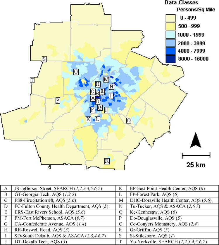
Map of twenty-county metropolitan Atlanta area with population density from 2000 census data. Letters reference monitor locations; the table identifies station name, network, and air pollutants monitored: 1=SO₂; 2=NO₂/NO_x; 3=CO; 4=O₃; 5=PM₁₀ mass; 6=PM_2.5 mass; 7=PM_2.5 composition (EC, OC, NO₃⁻, SO₄²⁻).

Data from five SO₂ monitors, six NO₂ and NO_x monitors, five CO monitors, five O₃ monitors, nine PM₁₀ monitors, eleven PM_2.5 monitors, and six PM_2.5 composition monitors were used in this study (Figure 1). In some cases, differences in the measurement methods employed by the different networks resulted in measurement bias. Slightly higher SO₂ values were obtained from the SEARCH monitors than the AQS monitors due to less SO₂ loss by condensation in the SEARCH sampling line. The SEARCH monitors have slightly lower NO_x measurements than the AQS monitors; for the SEARCH monitors, independent measurements of NO₂ and NO are summed, whereas the AQS measurement of total NO_x includes some NO_y species. The SEARCH PM₁₀ data used in this study were obtained by summing a filter-based Federal Reference Method (FRM) PM_2.5 measurement and a PM_coarse (PM₁₀ – PM_2.5) measurement obtained using a dichotomous sampler. The daily AQS PM₁₀ data at Georgia Tech, on the other hand, were obtained using a semi-continuous method. AQS PM₁₀ measurements taken every sixth day were obtained by FRM measurement. The SEARCH and AQS PM_2.5 data used are FRM measurements; the ASACA PM_2.5 measurements at Fort McPherson, South Dekalb and Tucker are TEOM measurements. For PM_2.5 EC/OC components, the SEARCH network measurement method is Thermal Optical Reflectance (TOR) whereas the ASACA and AQS measurements are by Thermal Optical Transmittance (TOT). The TOR method yields higher EC and lower OC than the TOT method.²⁹

Derivation of Population-Weighted Metrics

Air quality data, particularly primary pollutant data, tend to have a lognormal distribution.³⁰ To evaluate this, power transformations and Hinkley d_λ statistics were calculated for each pollutant at each monitor for λ = −0.5, 0, 0.5 and 1.³¹ Overall, an optimal power transformation of λ = 0 was found, indicating that the pollutant distributions are best described by a lognormal function.

In addition to being log-transformed, data were normalized:

$${\beta }_{i.k}=\frac{\ln (C_{i,k})-{\mu }_i}{{\sigma }_i}$$ (1)

Here, β_i,k is the normalized value of the pollutant at monitor i for day k, μ_i is the mean of ln(C_i,k) values for a year at monitor i, and σ_i is the standard deviation of ln(C_i,k) values for year at monitor i. Thus, the distribution of β_i has an annual mean of zero and an annual standard deviation of one. These normalized values were inverse distance-square weighted to the 660 census tracts as follows.

$$V_{j.k}=\frac{\sum _i{\beta }_{i.k}/D_{ij}^2}{\sum _{i}1/D_{ij}^2}$$ (2)

Here, V_j,k is the interpolated normalized value for each day k at each census tract j, and D_ij is the distance from monitor i to census tract j. Normalized values, as opposed to actual concentrations, were used to produce a smoother interpolated surface and increase the robustness of the metric when monitor data are missing. That is, without normalization, interpolation would result in average concentrations “floating” to regions where no monitors are located. In the case of a limited monitoring network of pollutants with concentrations that are much higher near the urban center than in surrounding rural areas (e.g. vehicular emission pollutants), direct interpolation would lead to unrealistic spatial distributions. The interpolation method used here is based entirely on the ambient monitor data and does not require the use of artificial boundary conditions. Moreover, without normalization the impact of missing data on these interpolations might be such that the results are only useful if data are available from all monitors. Such a reduction in completeness of the dataset might decrease substantially the power of a time-series health study.

The normalized value at each census tract was then converted back to a concentration using descriptive models of the means and standard deviations as a function of distance from the urban center.

$$C_{j,k}=e^{V_{j,k}{\sigma }_j+{\mu }_j}$$ (3)

Here, μ_j is the modeled mean of ln(C_j,k) values for the year at census tract j and σ_j is the modeled standard deviation of ln(C_j,k) values for the year at census tract j. Logistic and linear functions were used to model the annual means and standard deviations, respectively, providing a smooth spatial surface in which local source impacts and biases due to differences in measurement methods are minimized. This procedure allows for daily anisotropic pollutant fields, but the annual average pollutant fields (means and standard deviations) are assumed to be isotropic (i.e., dependent on radial distance only). This assumption has been assessed in previous work.³² The impact of prevailing wind direction on annual pollutant fields in the southeast is less pronounced than in other regions of the United States due to a relatively stagnant air mass, particularly in summer. After ambient air pollutant levels measured at an urban monitor and a rural monitor are described in the next section, spatial model fits of annual means and standard deviations are presented.

The final step was to population weight the concentrations in each census tract, resulting in an overall concentration to represent the study area for each day.

$$C_k=\frac{{\displaystyle \sum _j{C}_{j,k}{P}_j}}{{\displaystyle \sum _j{P}_j}}$$ (4)

Here, P_j is the population of census tract j, and C_k is the population-weighted concentration on day k. In a large population health study of the type being conducted in the twenty-county Atlanta metropolitan region, population-weighted metrics are likely to be more representative of exposure of the study population to ambient air pollution than data from a central monitor.

Urban and Rural Monitor Pollution Levels

Median and the 25–75% quartile range concentrations are given in Table 1 for daily measures of ambient pollutants from 1999 through 2004 at the Jefferson Street, Atlanta (urban) and at the Yorkville, Georgia (rural) SEARCH sites. Also shown is the urban-rural Pearson R² value. Primary pollutant concentrations are much higher at the urban site than the rural site. NO_x concentrations are about 10 times higher, CO concentrations are three to five times higher, and SO₂ and PM_2.5 EC concentrations are about twice as high, on average, at the urban site than at the rural site. Urban-rural SO₂ concentrations are less correlated than the other primary pollutant gases, consistent with the semivariogram analysis of Wade et al.³² Concentrations of secondary pollutants, on the other hand, are more uniform across the study area and are more correlated than concentrations of primary pollutants. Urban-to-rural average ratios for ozone and PM_2.5 sulfate and nitrate components are 0.85, 1.05 and 1.14, respectively; urban-rural R²-values for these secondary pollutants range from 0.635 to 0.844. PM₁₀ mass, PM_2.5 mass and PM_2.5 OC, which have both primary and secondary components, have urban-to-rural ratios ranging from 1.3 to 1.4 and have R²-values ranging from 0.350 to 0.725.

Table 1.

Air pollutant data at Jefferson Street and Yorkville, 1999–2004.

Pollutant	Jefferson St., Atlanta (urban)		Yorkville, GA (rural)		Pearson R2 (urban-rural)
	median	25–75% quartile range	median	25–75% quartile range
1-hr max NO2 (ppb)	42	31 – 52	8.2	5.0 – 14.3	0.025
1-hr max NOx (ppb)	86	49 – 166	8.9	5.3 – 15.5	0.050
1-hr max CO (ppb)	816	486 – 1,490	233	191 – 295	0.032
8-hr max O3 (ppb)	40	25 – 57	47	35 – 62	0.786
1-hr max SO2 (ppb)	12	6 – 24	6	4 – 11	0.009
avg PM10 (μg/m3)	25	19 – 34	19	13 – 28	0.600
avg PM2.5 (μg/m3)	16	11 – 21	12	8 – 17	0.725
avg PM2.5 ECa (μg/m3)	1.3	0.8 – 1.9	0.6	0.4 – 0.9	0.189
avg PM2.5 OCa (μg/m3)	3.8	2.7 – 5.3	2.7	1.9 – 4.0	0.350
avg PM2.5 NO3− (μg/m3)	0.7	0.4 – 1.3	0.6	0.4 – 1.1	0.634
avg PM2.5 SO42− (μg/m3)	3.9	2.4 – 6.1	3.7	2.2 – 6.4	0.844

^aTOR method

Spatial Distribution of Monitor Annual Means

For the retrospective health study in Atlanta, without detailed information about the location of subjects within the study area and with a limited number of monitors available for characterizing daily fluctuations in ambient pollutant levels, daily ambient pollutant metrics representative of the population were desired, as well as estimates of the uncertainty in the daily fluctuations based on spatial variability. The approach already described, which provides daily population-weighted concentrations as well as daily spatial distributions, requires that spatial means and standard deviations be modeled. Analysis of data on population and vehicle miles traveled (VMT) provides an indication of how pollutant concentrations may vary spatially. Data from the 2000 census, shown in Figure 2a, indicate an exponential decrease in population density with respect to distance from the urban center for the twenty-county Atlanta metropolitan area, defined here as the intersection of the north-south and east-west interstate highways (see Figure 3). The distribution of VMT might provide a better indicator of the spatial distribution of pollutants dominated by mobile source emissions, such as CO, NO₂/NO_x, and PM_2.5 EC. A plot of VMT density, generated using the Atlanta Regional Commission’s thirteen-county traffic demand model (calibrated for year 2000) which provides VMT estimates for over 38,000 roadway links,³³ shows a decrease in the log of VMT density with increase in distance from the urban center fitted with a logistic function (Figure 2b). VMT is high within the perimeter highway, which has a radius of approximately 20 km, and then decreases with increasing distance from the city center.

Figure 2.

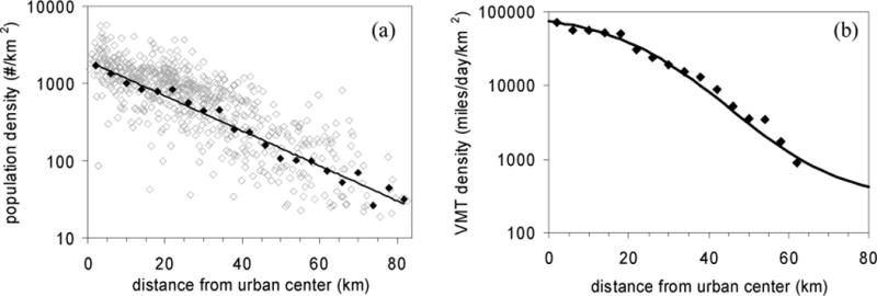
Population density (a) and VMT density (b) as a function of distance from urban center (as defined by the intersection of the north-south and east-west interstate highways). Hollow points represent 2000 census tract data in (a); solid points and regression results represent average population and VMT densities within concentric rings a distance of 4 km apart.

Figure 3.

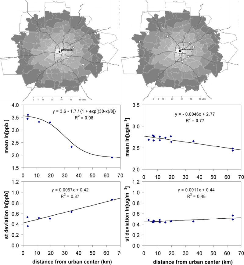
Spatial models of 2004 means and annual standard deviations of NO₂ (left three panels) and PM_2.5 (right three panels). The top panels show the locations of monitors (circles, black is central monitor, Jefferson Street), county boundaries (gray lines), zip codes (shaded), and interstate highways (dark lines). In 2004, there were six NO₂ monitors and twelve PM_2.5 monitors, including co-located instruments at two sites. The middle and bottom panels show the measured (points) and modeled (lines) annual means and standard deviations, respectively. Similar models were obtained in each of six years (1999–2004) for each of eleven pollutants.

Descriptive models of annual mean and standard deviation were fit for each year and for each pollutant. Two examples are shown in Figure 3: one-hour maximum NO₂ (left panels) and 24-hour average PM_2.5 mass (right panels), both in 2004. While the number of ambient monitors is limited (six for NO₂ and twelve for PM_2.5), the graphs suggest that the annual distributions of mean and standard deviation can be modeled with radial symmetry, consistent with previous work demonstrating the isotropic nature of correlations of pollutant measurements between pairs of monitors in the metropolitan Atlanta region.³² Similar models were obtained in each of six years (1999–2004) for each of eleven pollutants.

Results for all pollutants averaged over all years are shown in Figure 4. As expected, mean CO and NO₂/NO_x concentrations were best fit by logistic functions, whereas other pollutant concentrations were best fit by exponential functions. PM_2.5 EC was best fit by an exponential function, although the limited number of monitors and the difference in the measurement methods (TOR versus TOT) makes this assessment more subjective. Mean values of primary pollutants decreased much more than mean values of secondary pollutants with distance from the urban center, except for the primary pollutant SO₂. Sources of SO₂ are dominated by a few point sources of coal combustion emissions which are not located in the urban center.

Figure 4.

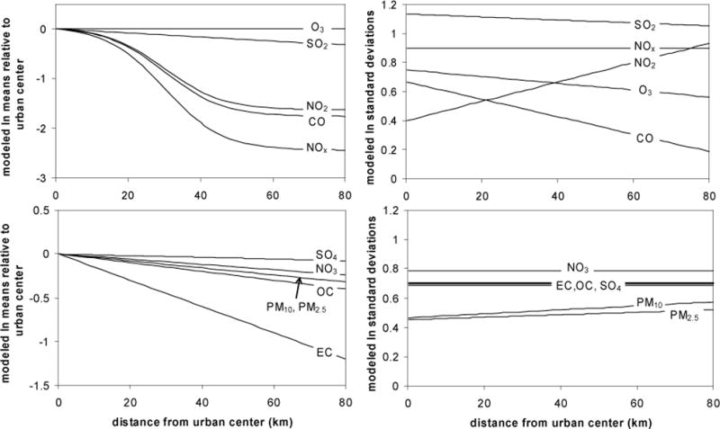
Modeled means relative to urban center (left) and standard deviations (right) of ln of pollutant concentrations as a function of distance from urban center.

The plots of standard deviation (right, Figure 4) demonstrate how annual variation differs over space. For the pollutants studied, annual variation is driven in large part by seasonal variation rather than day-to-day variation (e.g. day-of-week variation). Annual variation of SO₂ was greatest over the entire study area due to sporadic plume fumigation events. Variation in CO decreased most dramatically with distance from the urban center. CO from the oxidation of organics such as isoprene is a large contributor in rural areas, whereas CO from mobile source emissions is a large contributor in the urban center. The latter has a strong seasonal variation due to high emissions in winter from vehicle cold starts. NO₂ has a greater seasonal variation in rural areas than in the urban center, whereas NO has greater seasonal variation in the urban center. The four PM_2.5 components studied have greater variation than total PM_2.5 because these components have different seasonal profiles. EC, OC and NO₃ are highest in winter whereas SO₄ is highest in summer.

RESULTS

Population-Weighted Pollutant Concentrations

Calculated population-weighted concentrations and their variation (Figure 5) are found to be highly correlated (R>0.83) with data from the central monitor (Jefferson Street). However, population-weighted concentrations of primary pollutants are much lower than the central monitor data due to decreasing levels of these pollutants with increasing distance from the urban center.

Figure 5.

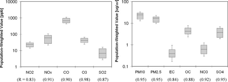
Box plots of the population-weighted pollutant values over the 1999–2004 study period. Dark lines indicate geometric means, shaded boxes indicate interquartile ranges, and extended lines with tails indicate standard deviations below and above the mean. R values with Jefferson Street monitor data are shown below axis.

In addition to calculating daily population-weighted pollutant concentrations, we have calculated daily population-weighted spatial variation as follows.

$$S_k={\displaystyle \sum _j\frac{{(C_{j,k}-{\overline{C}}_k)}^2{P}_j}{{\displaystyle \sum _j{P}_j}}}$$ (5)

Here, S_k is the daily population-weighted spatial variance of a pollutant and ${\overline{C}}_k$ is the average concentration on day k of all C_j,k. In a large population time-series health study in which population-weighted pollutant concentrations are used for exposure, population-weighted spatial variance is a measure of uncertainty in the exposure variable. Uncertainty in the exposure variable can lead to a bias to the null and a widening of the confidence interval in the estimation of health risk ratios.³⁴ Normalization of the spatial variation to the temporal (day-to-day) variation of population-weighted values indicates that the spatial variations of vehicle emission pollutants, that is NO₂, NO_x, CO and PM_2.5 EC, are high relative to their temporal variations (Figure 6). Since temporal variation provides the power with which to observe an association in a time-series health study, high values of the ratio of spatial variation to temporal variation would translate to low power in risk assessment. In a time-series study of the relationship of air pollution and acute health effects, these results suggest that using spatially resolved measures for these pollutants might provide better indicators of exposure.

Figure 6.

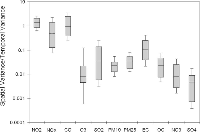
Box plots of the spatial variance normalized by the temporal variance over the 1999–2004 study period. Dark lines indicate geometric means, shaded boxes indicate interquartile ranges, and extended lines with tails indicate standard deviations below and above the mean.

Evaluation of Model Performance

The normalized bias (NBias) between monitor data (y_i) and calculated concentration values (x_i) at the census tract nearest the monitor is calculated using:

$$\text{NBias}=\frac{1}{\overline{y}}\frac{{\displaystyle \sum _{k=1}^N(y_k-x_k)}}{N}$$ (6)

The monitor data and calculated values are highly correlated, as expected, with R² values of 0.94 or greater for all pollutant measures. Lack of perfect correlation is due to the standard deviations not being perfectly modeled and the monitors not being located exactly at the zip code centroids. Bias is introduced by the smoothing of the mean and standard deviation profiles over space; results are shown in Figure 7. In many cases, this bias is desirable as it corrects for bias in measurement method or for local source impacts. A few examples are noted. The positive bias associated with the SEARCH NO_x calculation is due to different sampling protocol. The SEARCH monitors at Jefferson Street (A) and Yorkville (T) have negative biases for NO_x because they measure less NO_x than the AQS monitors that likely measure other oxides of nitrogen in addition to NO and NO₂. The SEARCH monitors have positive biases for SO₂ because they have less loss in sampling. The SEARCH monitors have a negative OC bias and positive EC bias due to the different temperature set points used by the TOR and TOT methods. Local source impacts are also observed. The South Dekalb monitor (I) is located near a major roadway, resulting in positive biases for NO_x and EC. Fire Station # 8 (C) is located near a railyard and a roadway with heavy diesel traffic; it has positive PM₁₀ and PM_2.5 biases.

Figure 7.

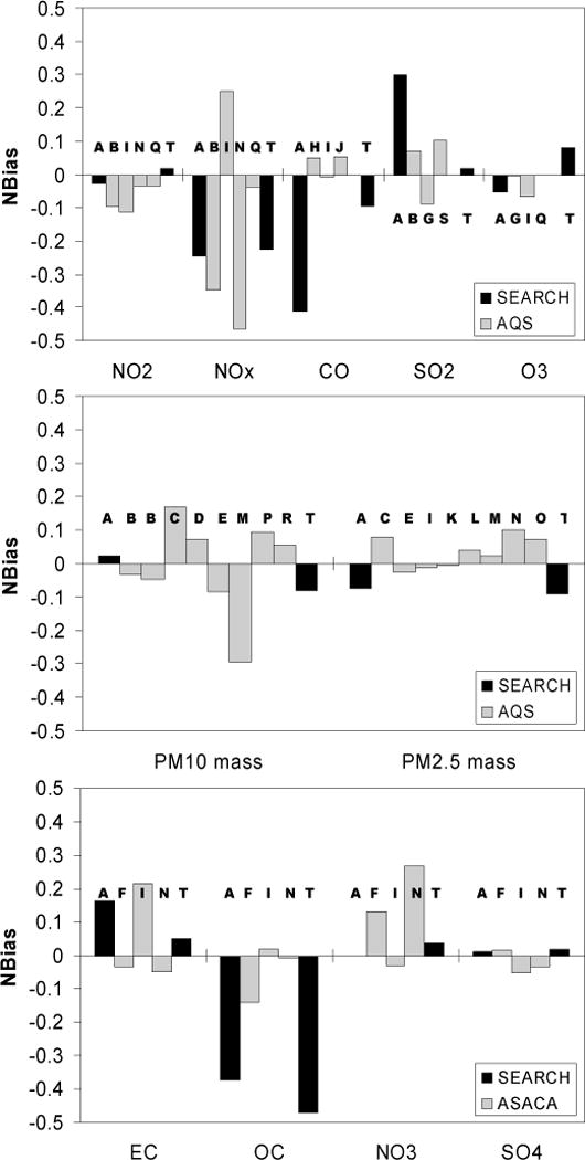
Normalized bias between monitor data and modeled values at the nearest census tract over the 1999–2004 period. Labels refer to monitors identified in Figure 1.

To evaluate model performance in predicting the spatial distribution of daily pollutant levels, the correlation of monitor observations and model predictions calculated without using data from that monitor are shown as a function of distance to the urban center in Figure 8. As distance from the urban center increases, the number of monitors decreases and the variability between monitors increases, resulting in decreasing predictive capability. For pollutants that are predominantly secondary in nature (i.e. formed in the atmosphere), such as ozone and PM_2.5 total and sulfate and nitrate component masses, high correlations (R > 0.8) are obtained even for sites within 65 km of the urban center. On the other hand, pollutants strongly associated with mobile sources, such as NO₂/NO_x, CO and PM_2.5-EC, are not well predicted at rural sites, with R values between 0.3 and 0.4 for the Yorkville site located approximately 64 km from the urban center. The ability to predict the SO₂ concentrations is particularly poor. Major sources of SO₂ in the Atlanta area are coal combustion point sources, in particular a coal-fired power plant located 11.5 km northwest of the urban center. When a plume from this plant impacts the Atlanta area, its width is narrow resulting in a spatially heterogeneous pollutant field that is not well characterized by the ambient monitors. The correlation of observations and predictions for PM_2.5-OC, which has significant primary and secondary components, is intermediate.

Figure 8.

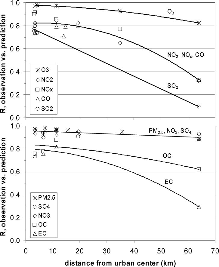
Correlation of monitor observations and model predictions without using data from that monitor as a function of distance from the urban center; top panel, pollutant gases; bottom panel, PM_2.5 total and major component masses. Curves indicate spatial trends for single pollutants or groups of pollutants. For co-located monitoring sites, both sets of observations were removed for model prediction at those sites. In the case of SO₂, observations at Stilesboro and Yorkville, located 63 and 64 km from the urban center respectively, were removed for prediction at this distance because the proximity of these two rural monitors (separated by 22 km) is atypical of rural monitors for other pollutants.

DISCUSSION

Assessment of Monitor Representativeness

To evaluate how representative of the study population the daily fluctuations of ambient air pollution at each monitor are, monthly correlations between the population-weighted metric and each monitor were calculated. Results, calculated as the average of the monthly Pearson R² values, indicate that data from stations closest to the urban center are most representative of (i.e. most correlated with) the population-weighted ambient level (Table 2). For primary pollutants, such as NO_x, CO, SO₂, and PM_2.5 EC, the correlations of the population-weighted values and the monitors greater than 50 km from the urban center are much lower than those for secondary pollutants, such as O₃ and PM_2.5 sulfate and nitrate.

Table 2.

Average of monthly correlations (Pearson R² values) between monitor data and population-weighted values, 1999–2004.

Distance	0–10 km					10–20 km				20–30 km	30–40 km	55–70 km
NO2	JS	GT				SD				Tu	Co		Yo
1-hr max	0.768	0.845				0.740				0.830	0.395		0.008
NOx	JS	GT				SD				Tu	Co		Yo
1-hr max	0.887	0.902				0.767				0.791	0.556		0.022
CO	JS					RR	SD	DT					Yo
1-hr max	0.787					0.656	0.759	0.765					0.073
O3	JS	CA				SD					Co		Yo
8-hr max	0.968	0.983				0.962					0.879		0.728
SO2	JS	GT	CA									St	Yo
1-hr max	0.800	0.743	0.754									0.091	0.020
PM 10	JS	GT-T	FS8	FC	ERS				DHC		Do	Gr	Yo
24-hr avg	0.904	0.912	0.628	0.653	0.720				0.659		0.514	0.568	0.630
PM 2.5	JS	FS8	ERS	FM		SD	EP	FP	DHC	Tu	Ke		Yo
24-hr avg	0.904	0.577	0.844	0.836		0.812	0.687	0.791	0.849	0.547	0.816		0.742
EC	JS	FM				SD1	SD2			Tu			Yo
24-hr avg	0.795	0.409				0.530	0.760			0.362			0.263
OC	JS	FM				SD1	SD2			Tu			Yo
24-hr avg	0.824	0.514				0.595	0.863			0.504			0.603
NO3	JS	FM				SD1	SD2			Tu			Yo
24-hr avg	0.824	0.569				0.429	0.813			0.481			0.499
SO4	JS	FM				SD1	SD2			Tu			Yo
24-hr avg	0.880	0.681				0.546	0.917			0.556			0.793

The low correlation of SO₂ measurements between the Jefferson Street (JS) monitor and monitors located nearby (Georgia Tech, GT, is 1.5 km from JS; Confederate Avenue, CA, is 8.3 km from JS) is due to the spatial heterogeneity of coal combustion plume impacts. The population-weighted CO values are less correlated with data from the Roswell Road (RR) monitor than data from either South Dekalb (SD) or Dekalb Tech (DT) despite RR being located nearer the urban center, likely due to nearby roadway emission impacts at RR. Finally, lower PM mass correlations are observed for the Fire Station # 8 (FS8) PM_2.5 and PM₁₀ monitors, possibly due to nearby railyard and roadway emission impacts at FS8.

These results provide a relative measure of the representativeness of ambient air quality monitors. Work is ongoing to convert these correlation values to error estimates and assess quantitatively the impact of this error on health risk assessment in terms of a bias to the null and widening of the confidence interval of risk ratio estimates.

Assessment of Completeness and Error Associated with Missing Data

To maximize completeness of the data set, it was desirable to compute the population-weighted average on days when data from some monitors were not available. This introduces error, but not bias, relative to the calculation using all monitor data available. To quantify this error, we used the method of data withholding to calculate the normalized root mean square error (NRMSE) associated with using data from different numbers of monitors:

$$\text{NRMSE}=\frac{1}{\overline{y}}\sqrt{\frac{{\displaystyle \sum _{k=1}^N{(y_k-x_k)}^2}}{N}}$$ (7)

Here, y_k are the daily population-weighted values calculated using data from all monitors, and x_k are these values calculated with data withheld. In Figure 9, results are shown for each pollutant as a function of the percentage of completeness of days when data are missing from 1999–2004. The total number of monitors and the percentage of total days with missing data are also given for each pollutant. For example, data were available from each of five SO₂ monitors located in the study area (three centrally located) on 1897 of 2192 days (85%) during the six-year study period (top graph, Figure 7). Population-weighted averages were calculated using available data with a NRMSE of 0.11 on 97 days of the 335 days with missing data (29%), with a NRMSE of 0.12 on 44 days (42% cumulative), with a NRMSE of 0.20 on 102 days (73% cumulative), and so on. On 7 days, or 2% of the 335 days with missing data, data from only one of the three centrally located SO₂ monitors were available and population-weighted averages were calculated with a NRMSE of 0.41.

Figure 9.

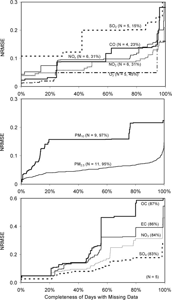
Normalized root mean square error associated with calculating population weighted average on days with data missing from one or more monitors. The total number of monitors (N) and the percentage of days for the 1999–2004 time period with data missing are shown in parentheses for each pollutant.

For pollutant gases, the largest error is associated with calculating population-weighted SO₂ concentrations on days when not all of the five SO₂ monitors report data, consistent with the finding of Wade et al.³² that the spatial distribution of ambient SO₂ in Atlanta is more poorly characterized than the other criteria pollutants. On the other hand, the lowest error is associated with calculating population-weighted O₃ concentrations on days when not all of the five O₃ monitors report data, except for some winter days when data from only the Yorkville monitor were available. For PM_2.5 components, the largest NRMSE is associated with EC and OC.

For use in time-series health studies, there is a tradeoff between maximizing exposure data completeness and minimizing exposure variable error. In health models that use a three-day moving average of a daily pollutant measure, which is the a priori model used in the Atlanta studies,^6,7 one missing day of a pollutant measure results in a loss of three days from the epidemiologic analysis, decreasing the statistical power to detect associations. On the other hand, the addition of error to the exposure measurement can result in loss of statistical power as well. Current work is quantitatively assessing these impacts on the risk ratio estimates.

CONCLUSION

A method for calculating population-weighted concentrations of ambient air pollution using data available from standard monitoring networks was developed and applied to the twenty-county Atlanta metropolitan area. The methodology results in a high correlation between monitor data and modeled estimates for the census tract where the monitor location (R₂ > 0.94), but allows for bias to dampen effects of measurement differences and local source impacts. This procedure allows for maximum completion of data sets for use in time-series health studies, with errors calculated for estimates performed with incomplete monitor data. In addition, the procedure allows for an assessment of the representativeness of ambient air pollutant monitors in a study area. Results are being used in ongoing investigations of the relationship between ambient air pollution and acute health effects in Atlanta.

References

- 1.Air Quality Criteria for Particulate Matter. EPA/600/P-99/002bB; U.S. Environmental Protection Agency; Washington, DC: Office of Research and Development, National Center for Environmental Assessment; Research Triangle Park, NC: 2001. [Google Scholar]
- 2.Dockery DW, Pope CA. Acute Respiratory Effects of Particulate Air Pollution. Annu Rev Public Health. 1994;15:107–132. doi: 10.1146/annurev.pu.15.050194.000543. [DOI] [PubMed] [Google Scholar]
- 3.Bascorn R, Bromberg PA, Costa DA, et al. Health Effects of Outdoor Air Pollution. Am J Respir Crit Care Med. 1996153:3–50. doi: 10.1164/ajrccm.153.1.8542133. [DOI] [PubMed] [Google Scholar]
- 4.Sarnet JM, Zeger SL, Dominici F, et al. The National Morbidity, Mortality, and Ambient Air Pollution Study Part II: Morbidity, Mortality, and Ambient Air Pollution in the United States. Cambridge, MA: Health Effects Institute; 2000. Research Report 94. [Google Scholar]
- 5.Brook RD, Franklin B, Cascio W, et al. Air Pollution and Cardiovascular Disease: A Statement for Health Care Professionals from the Expert Panel on Population and Prevention Science of the American Heart Association. Circulation. 2004;109:2655–2671. doi: 10.1161/01.CIR.0000128587.30041.C8. [DOI] [PubMed] [Google Scholar]
- 6.Metzger K, Tolbert P, Klein M, Peel J, Flanders WD, Todd K, Mulholland J, Ryan PB, Frumkin H. Ambient Air Pollution and Cardiovascular Emergency Department Visits. Epidemiology. 2004;15:46–56. doi: 10.1097/01.EDE.0000101748.28283.97. [DOI] [PubMed] [Google Scholar]
- 7.Peel J, Tolbert P, Klein M, Metzger K, Flanders WD, Todd K, Mulholland J, Ryan PB, Frumkin H. Ambient Air Pollution and Respiratory Emergency Department Visits. Epidemiology. 2005;16:164–174. doi: 10.1097/01.ede.0000152905.42113.db. [DOI] [PubMed] [Google Scholar]
- 8.Hernandez-Garduno E, Perez-Neria J, Paccagnella AM, Munguia-Castro M, Catalan-Vazquez M, Rojas-Ramos M. Air Pollution and Respiratory Health in Mexico City. Journal of Occupational and Environmental Medicine. 1997;39:299–307. doi: 10.1097/00043764-199704000-00006. [DOI] [PubMed] [Google Scholar]
- 9.von Klot S, Wolke G, Tuch T, Heinrich J, Dockery DW, Schwartz J, Kreyling WG, Wichmann HE, Peters A. Increased asthma medication use in association with ambient fine and ultrafine particles. European Respiratory Journal. 2002;20:691–702. doi: 10.1183/09031936.02.01402001. [DOI] [PubMed] [Google Scholar]
- 10.Linn WS, Szlachcic Y, Gong H, Jr, Kinney PL, Berhane KT. Air Pollution and Daily Hospital Admissions in Metropolitan Los Angeles. Environmental Health Perspectives. 2000;108:427–434. doi: 10.1289/ehp.00108427. [DOI] [PMC free article] [PubMed] [Google Scholar]
- 11.Katsouyanni K, Zmirou D, Spix C, Sunyer J, Schouten JP, Ponka A, Anderson HR, Le Moullec Y, Wojtyniak B, Vigotti MA, Bacharova L. Short-term effects of air pollution on health: a European approach using epidemiological time-series data. European Respiratory Journal. 1995;8:1030–1039. [PubMed] [Google Scholar]
- 12.Burnett RT, Cakmak S, Raizenne ME, Stieb D, Vincent R, Krewski D, Brook JR, Philips O, Ozkaynak H. The Associations between Ambient Carbon Monoxide Levels and Daily Mortality in Toronto, Canada. Journal of Air & Waste Management Association. 1998;48:689–700. doi: 10.1080/10473289.1998.10463718. [DOI] [PubMed] [Google Scholar]
- 13.von Klot S, Peters A, Aalto P, Bellander T, Berglind N, D’Ippoliti D, Elosua R, Hormann A, Kulmala M, Lank T, Lowel H, Pekkanen J, Picciotto S, Sunyer J, Forastiere F. Ambient Air Pollution Is Associated With Increased Risk of Hospital Cardiac Readmissions of Myocardial Infarction Survivors in Five European Cities. Circulation. 2005;112:3073–3079. doi: 10.1161/CIRCULATIONAHA.105.548743. [DOI] [PubMed] [Google Scholar]
- 14.Marshall JD, Riley WJ, McKone TE, Nazaroff WW. Intake fraction of primary pollutants: motor vehicle emissions in the South Coast Air Basin. Atmospheric Environment. 2003;37:3455–3468. [Google Scholar]
- 15.Mulholland JA, Butler AJ, Wilkinson JG, Russell AG, Tolbert PE. Temporal and Spatial Distributions of Ozone in Atlanta: Regulatory and Epidemiological Implications. Journal of Air & Waste Management Association. 1998;48:418–426. doi: 10.1080/10473289.1998.10463695. [DOI] [PubMed] [Google Scholar]
- 16.Tolbert PE, Mulholland JA, Macintosh DL, Xu F, Daniels D, Devine OJ, Carlin BP, Klein M, Dorley J, Butler AJ, Nordenberg DF, Frumkin H, Ryan PB, White MC. Air Quality and Pediatric Emergency Room Visits for Asthma in Atlanta, Georgia. American Journal of Epidemiology. 2000;151:798–810. doi: 10.1093/oxfordjournals.aje.a010280. [DOI] [PubMed] [Google Scholar]
- 17.Buzzelli M, Jerrett M, Burnett R, Finklestein N. Spatiotemporal Perspectives on Air Pollution and Environmental Justice in Hamilton, Canada, 1985–1996. Annals of the Association of American Geographers. 2003;93:557–573. [Google Scholar]
- 18.English P, Neutra R, Scalf R, Sullivan M, Waller L, Zhu L. Examining Associations between Childhood Asthma and Traffic Flow Using a Geographic Information System. Environmental Health Perspectives. 1999;107:761–767. doi: 10.1289/ehp.99107761. [DOI] [PMC free article] [PubMed] [Google Scholar]
- 19.Wilkinson P, Elliott P, Grundy C, Shaddick G, Thakrar B, Walls P, Falconer S. Case-control study of hospital admission with asthma in children aged 5–14 years: relation with road traffic in north west London. Thorax. 1999;54:1070–1074. doi: 10.1136/thx.54.12.1070. [DOI] [PMC free article] [PubMed] [Google Scholar]
- 20.Buckeridge DL, Glazier R, Harvey BJ, Escobar M, Amrhein C, Frank J. Effect of Motor Vehicle Emissions on Respiratory Health in an Urban Area. Environmental Health Perspectives. 2002;110:293–300. doi: 10.1289/ehp.02110293. [DOI] [PMC free article] [PubMed] [Google Scholar]
- 21.Hoek G, Brunekreef B, Goldbohm S, Fischer P, van den Brandt PA. Associations between mortality and indicators of traffic-related air pollution in the Netherlands: a cohort study. Lancet. 2002;360:1203–1209. doi: 10.1016/S0140-6736(02)11280-3. [DOI] [PubMed] [Google Scholar]
- 22.Briggs DJ, Collins S, Elliott P, Fischer P, Kingham S, Lebret E, Pryl K, Van Reeuwijk H, Smallbone K, Van der Veen A. Mapping urban air pollution using GIS: a regression-based approach. Int J Geographical Information Science. 1997;11:699–718. [Google Scholar]
- 23.Gilbert NL, Goldberg MS, Beckerman B, Brook JR, Jerrett M. Assessing Spatial Variability of Ambient Nitrogen Dioxide in Montreal, Canada, with a Land-Use Regression Model. Journal of Air & Waste Management Association. 2005;55:1059–1063. doi: 10.1080/10473289.2005.10464708. [DOI] [PubMed] [Google Scholar]
- 24.Jerrett M, Arain A, Kanaroglou P, Beckerman B, Potoglou D, Sahsuvaroglu T, Morrison J, Giovis C. A review and evaluation of intraurban air pollution exposure models. Journal of Exposure Analysis and Environmental Epidemiology. 2005;15:185–204. doi: 10.1038/sj.jea.7500388. [DOI] [PubMed] [Google Scholar]
- 25.Tong DQ, Mauzerall DL. Spatial variability of summertime tropospheric ozone over the continental United States: Implications of an evaluation of the CMAQ model. Atmospheric Environment. 2006;40:3041–3056. [Google Scholar]
- 26.Hansen DA, Edgerton E, Hartsell B, Jansen J, Burge H, Koutrakis P, Rogers C, Suh H, Chow J, Zielinska B, McMurry P, Mulholland J, Russell A, Rasmussen R. Air quality measurements for the aerosol research and inhalation epidemiology study. Journal of the Air & Waste Management Association. 2006;56:1445–1458. doi: 10.1080/10473289.2006.10464549. [DOI] [PubMed] [Google Scholar]
- 27.Butler AJ, Andrew MS, Russell AG. Daily sampling of PM2.5 in Atlanta: results of the first year of the assessment of spatial aerosol composition in Atlanta study. Journal of Geophysical Research-Atmospheres. 2003;108:8415. [Google Scholar]
- 28.U.S. EPA. Implementation Plan: PM2.5 Monitoring Program. available at http://www.epa.gov/ttn/amtic/files/ambient/pm25/pmplan3.pdf (accessed 2007).
- 29.Chow JC, Watson JG, Crow D, Lowenthal DH, Merrifield T. Comparison of IMPROVE and NIOSH carbon measurements. Aerosol Sci Technol. 2001;34:23–34. [Google Scholar]
- 30.Ott WR. A Physical Explanation of the Lognormality of Pollutant Concentrations. Journal of the Air & Waste Management Association. 1990;40:1378–1383. doi: 10.1080/10473289.1990.10466789. [DOI] [PubMed] [Google Scholar]
- 31.Wilks DS. Statistical Methods in the Atmospheric Sciences. Vol. 91. Elsevier Science and Technology; San Diego: 2005. pp. 21–63. [Google Scholar]
- 32.Wade KS, Mulholland JA, Marmur A, Russell AG, Hartsell B, Edgerton E, Klein M, Waller L, Peel JL, Tolbert PE. Instrument Error and Spatial Variability of Ambient Air Pollution in Atlanta, Georgia. Journal of Air & Waste Management Association. 2006;56:876–888. doi: 10.1080/10473289.2006.10464499. [DOI] [PubMed] [Google Scholar]
- 33.Atlanta Regional Commission (ARC) Atlanta’s Traffic Model. available at http://atlantaregional.com/html/357_ENU_HTML.htm (accessed 2007).
- 34.Zeger SL, Thomas D, Dominici F, Samet JM, Schwartz J, Dockery D, Cohen A. Exposure measurement error in time-series studies of air pollution: concepts and consequences. Environ Health Perpectives. 2000;108:419–426. doi: 10.1289/ehp.00108419. [DOI] [PMC free article] [PubMed] [Google Scholar]