A Tutorial on Adaptive Design Optimization

Abstract

Experimentation is ubiquitous in the field of psychology and fundamental to the advancement of its science, and one of the biggest challenges for researchers is designing experiments that can conclusively discriminate the theoretical hypotheses or models under investigation. The recognition of this challenge has led to the development of sophisticated statistical methods that aid in the design of experiments and that are within the reach of everyday experimental scientists. This tutorial paper introduces the reader to an implementable experimentation methodology, dubbed Adaptive Design Optimization, that can help scientists to conduct “smart” experiments that are maximally informative and highly efficient, which in turn should accelerate scientific discovery in psychology and beyond.

1 Introduction

Imagine an experiment in which each and every stimulus was custom tailored to be maximally informative about the question of interest, so that there were no wasted trials, participants, or redundant data points. Further, what if the choice of design variables in the experiment (e.g., stimulus properties and combinations, testing schedule, etc.) could evolve in real-time as data were collected, to take advantage of information about the response the moment it is acquired (and possibly alter the course of the experiment) rather than waiting until the experiment is over and then deciding to conduct a follow-up?

The ability to fine-tune an experiment on the fly makes it possible to identify and capitalize on individual differences as the experiment progresses, presenting each participant with stimuli that match a particular response pattern or ability level. More concretely, in a decision making experiment, each participant can be given choice options tailored to her or his response preferences, rather than giving every participant the same, pre-selected list of choice options. As another example, in an fMRI experiment investigating the neural basis of decision making, one could instantly analyze and evaluate each image that was collected and adjust the next stimulus accordingly, potentially reducing the number of scans while maximizing the usefulness of each scan.

The implementation of such idealized experiments sits in stark contrast to the current practice in much of psychology of using a single design, chosen at the outset, throughout the course of the experiment. Typically, stimulus creation and selection are guided by heuristic norms. Strategies to improve the informativeness of an experiment, such as creating all possible combinations of levels of the independent variables (e.g., three levels of task difficulty combined with five levels of stimulus duration), actually work against efficiency because it is rare for all combinations to be equally informative. Making matters worse, equal numbers of participants are usually allotted to each combination of treatments for statistical convenience, even the treatments that may not be informative. Noisy data are often combatted in a brute-force way by simply collecting more of them (this is the essence of a power analysis). The continued use of these practices is not the most efficient use of time, money, and participants to collect quality data.

A better, more efficient way to run an experiment would be to dynamically alter the design in response to observed data. The optimization of experimental designs has a long history in statistics dating back to the 1950s (e.g., Lindley, 1956; Box and Hill, 1967; Atkinson and Federov, 1975; Atkinson and Donev, 1992; Berry, 2006). Psychometricians have been doing this for decades in computerized adaptive testing (e.g., Weiss and Kingsbury, 1984), and psychophysicists have developed their own adaptive tools (e.g., Cobo-Lewis, 1997; Kontsevich and Tyler, 1999). The major hurdle in applying adaptive methodologies more broadly has been computational: Quantitative tools for identifying the optimal experimental design when testing formal models of cognition have not been available. However, recent advances in statistical computing (Doucet et al., 2001; Robert and Casella, 2004) have laid the groundwork for a paradigmatic shift in the science of data collection. The resulting new methodology, dubbed adaptive design optimization (ADO, Cavagnaro et al., 2010), has the potential to more broadly benefit experimentation in cognitive science and beyond.

In this tutorial, we introduce the reader to adaptive design optimization. The tutorial is intended to serve as a practical guide to apply the technique to simple cognitive models. As such, it assumes a rudimentary level of familiarity with cognitive modeling, such as how to implement quantitative models in a programming or graphical language, how to use maximum likelihood estimation to determine parameter values, and how to apply model selection methods to discriminate models. Readers with little familiarity with these techniques might find Section 3 difficult to follow, but should otherwise be able to understand most of the other sections. We begin by reviewing approaches to improve inference in cognitive modeling. Next we describe the technical details of adaptive design optimization, covering the computational and implementation details. Finally, we present an example application of the methodology for designing experiments to discriminate simple models of memory retention. Readers interested in more technical treatments of the material should consult (Myung and Pitt, 2009; Cavagnaro et al., 2010).

2 Why Optimize Designs?

2.1 Not All Experimental Designs Are Created Equal

To illustrate the importance of optimizing experimental designs, suppose that a researcher is interested in empirically discriminating between formal models of memory retention. The topic of retention has been studied for over a century. Years of research have shown that a person’s ability to remember information just learned drops quickly for a short time after learning and then levels off as more and more time elapses. The simplicity of this data pattern has led to the introduction of numerous models to describe the change over time in the rate at which information is retained in memory. Through years of experimentation with humans (and animals), a handful of the models have proven to be superior to the rest of the field (Wixted and Ebbesen, 1991), although more recent research suggests that they are not complete (Oberauer and Lewandowsky, 2008). These models describe the probability p of correctly recalling a stimulus item as a function of the time t since study. Two particular models that have received considerable attention are the power model, p = a(t + 1)^−b, and the exponential model, p = ae^−bt. Both models predict that memory recall decays gradually as the lag time between study and test phases increases.

Figure ?? shows predictions of power and exponential models obtained under restricted ranges of parameter values (i.e., 0.65 < a < 0.85 and 0.75 < b < 0.95 for the power model, and 0.80 < a < 1.00 and 0.10 < b < 0.20 for exponential model). Suppose that the researcher conducts an experiment to compare these model predictions by probing memory at different lag times, which represent values of a design variable in this experiment. Visual inspection of the figure suggests that lag times between 15 and 20 seconds would be bad designs to use because in this region predictions from both models are virtually indistinguishable from each other. In contrast, times between 1 and 5 seconds, where the models are separated the most, would make good designs for the model discrimination experiment.

In practice, however, the problem of identifying good designs is a lot more complicated than the idealized example in Figure ??. It is more often the case that the researchers have little information about the specific ranges or values of model parameters under which experimental data are likely to be observed. Further, the models under investigation may have many parameters so visual inspection of their predictions across designs would be simply impossible. This is where quantitative tools for optimizing designs can help identify designs that make experiments more efficient and more effective than what is possible with current practices in experimental psychology. In the remainder of this tutorial, we will describe how the optimization of designs can be accomplished. For an illustrative application of the methodology for discriminating the aforementioned models of retention, the reader may skip ahead to Section 4.

2.2 Optimal Design

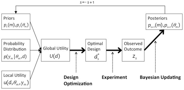
In psychological inquiry, the goal of the researcher is often to distinguish between competing explanations of data (i.e., theory testing) or to estimate characteristics of the population along certain psychological dimensions, such as the prevalence and severity of depression. In cognitive modeling, these goals become ones of model discrimination and parameter estimation, respectively. In both endeavors, the aim is to make the strongest inference possible given the data in hand. The scientific process is depicted inside in the rectangle in Figure ??a: first, the values of design variables are chosen in an experiment, then the experiment is carried out and data are collected, and finally, data modeling methods (e.g., maximum likelihood estimation, Bayesian estimation) are applied to evaluate model performance at the end of this process.

Over the last several decades, significant theoretical and computational advances have been made that have greatly improved the accuracy of inference in model discrimination (e.g., Burnham and Anderson, 2010). Model selection methods in current use include the Akaike Information Criterion (Akaike, 1973), the Bayes factor (Jeffreys, 1961; Kass and Raftery, 1995), and Minimum Description Length (Rissanen, 1978; Grünwald, 2005), to name a few. In each of these methods, a model’s fit to the data is evaluated in relation to its overall flexibility in fitting any data pattern, to arrive at a decision regarding which model of two competing models to choose (Pitt et al., 2002). As depicted in in Figure ??a, data modeling is applied to the back end of the experiment after data collection is completed. Consequently, the methods themselves are limited by the quality of the empirical data collected. Inconclusive data will always be inconclusive, making the task of model selection difficult no matter what data modeling method is used. A similar problem presents itself in estimating model parameters from observed data, regardless of whether maximum likelihood estimation or Bayesian estimation is used.

Because data modeling methods are not foolproof, attention has begun to focus on the front end of the data collection enterprise, before an experiment is conducted, developing methods that optimize the experimental design itself. Design optimization (DO, Myung and Pitt, 2009) is a statistical technique, analogous to model selection methods, that selectively chooses design variables (e.g., treatment levels and values, presentation schedule) with the aim of identifying an experimental design that will produce the most informative and useful experimental outcome (Atkinson and Donev, 1992). Because experiments can be difficult to design, the consequences of design choices and the quality of the proposed experiment are not always predictable, even if one is an experienced researcher. DO can remove some of the uncertainty of the design process by taking advantage of the fact that both the models and some of the design variables can be quantified mathematically.

How does DO work? To identify an optimal design, one must first define the design space, which consists of the set of all possible values of design variables that are directly controlled by the experimenter. The researcher must define this set by considering the properties of the variables being manipulated. For example, a variable on an interval scale may be discretized. The coarser the discretization, the fewer the number of designs. Given five design variables, each with ten levels, there are 100,000 possible designs.

In addition, the model being evaluated must be expressed in formal, mathematical terms, whether it is a model of visual processing, recognition memory, or decision making. A mathematical framework provided by Bayesian decision theory (Chaloner and Verdinelli, 1995) offers a principled approach to design optimization. Specifically, each potential design is viewed as a gamble whose payoff is determined by the outcome of an experiment conducted with that design. The payoff represents some measure of the goodness or the utility of the design. Given that there are many possible outcomes that an experiment could produce, one estimates the expected utility (i.e., predicted utility) of a given design by computing the average payoffs across all possible outcomes that could be observed in an experiment carried out with the chosen design. The design with the highest expected utility is then identified as the optimal design. To conceptualize the problem slightly differently, if one imagines a distribution representing the utility of all designs, ordered from worst to best, the goal of DO is to identify the design at the extreme (best) endpoint of the distribution.

2.3 An Adaptive Approach to Experimentation: Adaptive Design Optimization

DO is a one-shot process. An optimal design is identified, applied in an experiment, and then data modeling methods are used to aid in interpreting the results, as depicted in Figure ??a,. This inference process can be improved by using what is learned about model performance in the data modeling stage to optimize the design still further. Essentially, these two stages are connected as shown in Figure ??b, yielding adaptive design optimization (ADO).

ADO is an integrative approach to experimentation that leverages, online, the complementary strengths of design optimization and data modeling. The result is an efficient and informative method of scientific inference. In ADO, the optimal experimental design is updated at intervals during the experiment, which we refer to as stages. It can be as frequent as after every trial or after a number of trials (e.g., a mini experiment). Factors such as the experimental methodology being used will influence the frequency of updating. As depicted in Figure ??b, updating involves repeating data modeling and design optimization. More specifically, within a Bayesian framework, adaptive design optimization is cast as a decision problem where, at the end of each stage, the most informative design for the next stage (i.e., the design with the highest expected utility) is sought based on the design and outcomes of the previous stage. This new stage is then carried out with that design, and the resulting data are analyzed and modeled. This is followed by identifying a new design to be used in the next stage.¹ This iterative process continues until an appropriate stopping criterion is reached.

Various additional (pragmatic) decisions arise with ADO. In particular, one must decide how many mini experiments will be carried out, either in succession within a single testing session (e.g., one hour). A critical factor, which is likely only determined with piloting, is how many stages are necessary to obtain decisive model discrimination or stable parameter estimation. It may be that testing would be required across days, but to date we have not found this to be necessary.

By using all available information about the models and how the participant has responded, ADO collects data intelligently. It has three attractive properties that make it particularly well suited for evaluating computational models. These pertain to the informativeness of the data collected in the experiment, the sensitivity of the method to individual differences, and the efficiency of data collection. We briefly elaborate on each.

As noted above, design optimization and data modeling are synergistic techniques that are united in ADO to provide a clear answer to the question of interest. Each mini-experiment is designed, or each trial chosen, such that the evidence pertaining to the question of interest, whether it be estimating a participant’s ability level or discriminating between models, accumulates as rapidly as possible. This is accomplished by using what is learned from each stage to narrow in on those regions of the design space that will be maximally informative in some well-defined sense.

The adaptive nature of the methodology, by construction, controls for individual differences and thus makes it well suited for studying the most common and often largest source of variance in experiments. When participants are tested individually using ADO, the algorithm adjusts (i.e., optimizes) the design of the experiment to the performance of that participant, thereby maximizing the informativeness of the data at an individual participant level. Response strategies and group differences can be readily identified. This capability also makes ADO ideal for studies in which few participants can be tested (e.g., rare memory or language disorders).

Another benefit of using an intelligent data collection scheme is that it speeds up the experiment, possibly resulting in a substantial savings of time, fewer trials and participants, and lower cost. This savings can be significant when using expensive technology (e.g., fMRI) or numerous support staff (e.g., developmental or clinical research). Similarly, in experiments using hard-to-recruit populations (children, elderly, mental patients), application of ADO means fewer participants, all without sacrificing the quality of the data or the quality of the statistical inference.

The versatility and efficiency of ADO has begun to attract attention in various disciplines. It has been used recently for designing neurophysiology experiments (Lewi et al., 2009), adaptive estimation of contrast sensitivity functions of human vision (Kujala and Lukka, 2006; Lesmes et al., 2006, 2010; Vul and Bergsma, 2010), designing systems biology experiments (Kreutz and Timmer, 2009), detecting exoplanets in astronomy (Loredo, 2004), conducting sequential clinical trials (e.g., Wathen and Thall, 2008), and adaptive selection of stimulus features in human information acquisition experiments (Nelson, 2005; Nelson et al., 2011). Perhaps the most well-known example of ADO, albeit a very different implementation of it, is computerized adaptive testing in psychology (e.g., Hambleton et al., 1991; van der Linden and Glas, 2000). Here, an adaptive sequence of test items, which can be viewed in essence as experimental designs, is chosen from an item bank taking into account an examinee’s performance on earlier items so as to accurately infer the examinee’s ability level with the fewest possible items.

In our lab, we have used ADO to adaptively infer a learner’s representational state in cognitive development experiments (Tang et al., 2010), to discriminate models of memory retention (Cavagnaro et al., 2010, 2011), and to optimize risky decision making experiments (Cavagnaro et al., 2013a,b). These studies have clearly demonstrated the superior efficiency of ADO to the alternative non-ADO methods, such as random and fixed designs (e.g., Cavagnaro et al., 2010, 2013a, Fig. 3 & Fig. 7, respectively).

Figure 3.

Schematic illustration of the steps involved in adaptive design optimization (ADO).

Figure 7.

Heat map of the data-generating model in the ADO simulation. Darker colors indicate regions of higher probability.

3 The Nuts and Bolts of Adaptive Design Optimization

In this section we describe the theoretical and computational aspects of ADO in greater detail. The section is intended for readers who are interested in applying the technique to their own cognitive modeling. Our goal is to provide readers with the basic essentials of implementing ADO in their own experiments. Figure ?? show a schematic diagram of the ADO framework that involves a series of steps. In what follows we discuss each step in turn.

3.1 Preliminaries

Application of ADO requires that each model under consideration be formulated as a statistical model defined as a parametric family of probability distributions, p(y|θ, d)’s, each of which specifies the probability of observing an experimental outcome (y) given a parameter value (θ) and a design value (d). That is, the data vector y is a sample drawn from the probability distribution (often called the sampling distribution) for given values of the parameter vector θ and of the design vector d.

To be concrete, consider the exponential model of memory retention, defined by p = ae^−bt, that describes the probability of correct recall of a stimulus item (e.g., word or picture) as a function of retention interval t and parameter vector θ = (a, b) where 0 < a < 1 and b > 0. In a typical experiment, there is a study phase in which participants learn a list of words. After a retention interval, which can range from fractions of a second to minutes, participants are tested on their memory for the list of words. Data are scored as the number of correctly recalled items (y) out of a fixed number of independent Bernoulli trials (n), all given at a single retention interval t. Note that the retention interval is the design variable whose value is being experimentally manipulated, i.e., d = t.

Under the assumption that the exponential model describes retention performance, the experimental outcome would follow the binomial probability distribution of the form

$$p(y\mid \theta =(a,b),t)=\frac{n!}{(n-y)!y!}{\left({ae}^{-bt}\right)}^y{\left(1-{ae}^{-bt}\right)}^{n-y},$$ (1)

where y = 0, 1, …, n. When retention performance is probed over multiple time points of the design variable, d = (t₁, …, t_q ), the data are summarized into a discrete vector y = (y₁, …, y_q ) with each y_i ∈ {0, …, n}, and the overall probability distribution of the outcome vector y is then given by

$$p(y\mid \theta =(a,b),d)=\prod _{i=1}^q\frac{n!}{(n-y_i)!y_i!}{\left({ae}^{-{bt}_i}\right)}^{y_i}{\left(1-{ae}^{-{bt}_i}\right)}^{n-y_i}.$$ (2)

ADO is formulated in a Bayesian statistical framework. It is beyond the scope of this tutorial to review this vast literature, and instead, the reader is directed to consult Bayesian textbooks (e.g., Robert, 2001; Gelman et al., 2004; Gill, 2007; Kruschke, 2010). The Bayesian formulation of ADO requires specification of priors for model parameters, denoted by p(θ). There are a plethora of methods proposed in the Bayesian literature for choosing appropriate priors, whether they are subjective, objective, or empirical priors (Carlin and Louis, 2000, for a review). Practically speaking, however, what is important to note is that ADO results might strongly depend upon the particular form of the prior employed so it must be chosen with careful thought and proper justification.

As a concrete example, for the above two parameters, a and b, of the exponential model of retention, one might choose to employ the following prior defined by the product of a Beta probability density for parameter a and an exponential probability density for parameter b

$$p(\theta =(a,b))=\frac{\mathrm{\Gamma }(\alpha +\beta )}{\mathrm{\Gamma }(\alpha )\mathrm{\Gamma }(\beta )}{a}^{\alpha -1}{(1-a)}^{\beta -1}\lambda e^{-\lambda b},$$ (3)

for α = 4, β = 2, and λ = 10, for instance. Combining the prior distribution in the above equation with the probability distribution of the outcome vector in Eq. (2) by Bayes rule yields the posterior distribution as

$$p(\theta =(a,b)\mid y,d)=\frac{p(y\mid \theta =(a,b),d)p(\theta =(a,b))}{\int \int p(y\mid \theta =(a,b),d)p(\theta =(a,b))\mathit{dadb}}.$$ (4)

Having specified a model’s probability distribution and the prior and posterior distributions of model parameters, we now discuss the details of the ADO framework

3.2 Design Optimization

As mentioned earlier, ADO is a sequential process consisting of a series of optimization-experimentation stages. An optimal design is sought on the basis of the present state of knowledge, which is coded in the prior. Next, data are collected with the optimal design. The observed outcomes are then used to update the prior to the posterior, which in turn becomes the prior on the next iteration of the ADO process. As such, the design is optimized in each ADO stage, and this design optimization (DO) step involves solving an optimization problem defined as

$$d^{\ast }=\underset{d}{\text{argmax}}U(d),$$ (5)

for some real-valued function U (d) that is a metric of goodness or utility of design d.

Formally and without loss of generality, we define the utility function U (d) to be optimized as

$$U(d)=\sum _{m}p(m)\int \int u(d,{\theta }_m,y_m)p(y_m\mid {\theta }_m,d)p({\theta }_m){dy}_{m}d{\theta }_m,$$ (6)

where m = {1, 2, …, K} is one of a set of K models being considered, and y_m is the outcome vector resulting from a hypothetical imaginary experiment, in lieu of a real one, conducted with design d under model m, and θ_m is a parameter vector of model m (e.g., Chaloner and Verdinelli, 1995; Myung and Pitt, 2009; Nelson et al., 2011). In the above equation, p(m) denotes the prior model probability of model m. The “local” utility function, u(d, θ_m, y_m), measures the utility of an imaginary experiment carried out with design d when the data generating model is m, the parameters of the model take the value θ_m, and the outcome y_m is produced.

On the left side of the above equation is what is sometimes referred to as the global utility function U (d) (so as to distinguish it from the local utility function defined above), and is defined as the expectation of u(·) averaged over the models, parameters, and observations, taken with respect to the model prior p(m), the parameter prior p(θ_m), and the probability distribution p(y_m|θ_m, d), respectively.

To evaluate the global utility U (d) in Eq. (6), one must provide explicit specifications for three functions: (1) the model and parameter priors, p(m) and p(θ_m); (2) the probability distribution given parameter θ_m and design d, p(y_m|θ_m, d); and (3) the local utility function u(d, θ_m, y_m). These are shown on the left side of Figure ??, which is a schematic illustration of ADO. The first two functions were discussed in the preceding section. We discuss the specification of the third, the local utility function, next.

3.3 Local Utility Function

From Eq. (5), it can be seen that the global utility being optimized is nothing but an average value of the local utility over all possible data samples and model parameters, weighted by the likelihood function and the model and parameter priors. As such, selection of a local utility function in ADO determines the characteristics of what constitutes an optimal design. One should therefore choose a local utility function that is appropriate for the specific goal of the experiment.

Generally speaking, the cognitive modeler conducts an experiment with one of two goals in mind: parameter estimation or model discrimination. In parameter estimation, given a model of interest, the goal is to estimate the values of the model’s parameters as accurately as possible with the fewest experimental observations. On the other hand, in model discrimination, given a set of multiple candidate models, the goal is to identify the one that is closest in some defined sense to the underlying data generating model, again using the fewest number of observations. Below we discuss possible forms of the local utility function one can use for either goal.

A simple and easy-to-understand local utility function for parameter estimation is of the following form:

$$u(d,\theta =({\theta }_1,\dots ,{\theta }_k),y)=\sum _{i=1}^k\frac{E({\theta }_i)}{SD({\theta }_i)},$$ (7)

where k is the number of parameters, and E(θ_i) and SD(θ_i) stand for the mean and standard deviation, respectively, of the posterior distribution of parameter θ_i, denoted as p(θ_i|y, d). Note that by construction, K in Eq. (6) is equal to 1 in parameter estimation so the subscript m is skipped in Eq. (7). The above local utility function is defined as a sum of “inverse” standard deviations of parameters weighted by their means so that the function value does not depend upon the unit in which each parameter is measured. Note that a larger value of u(d, θ, y) is translated into less parameter variability overall, which in turn implies a more accurate estimate of the parameters. One may also consider other variations of the above form, each suitably chosen taking into account the particular purpose of the experiment at hand.

Sometimes, the choice of a local utility function can be driven by the principled choice of a global utility function. Perhaps the most commonly employed global utility function in the literature is the following, motivated from information theory:

$$U(d)=I(\mathrm{\Theta };Y\mid d)$$ (8)

which is the mutual information between the parameter random variable Θ and the outcome random variable Y conditional upon design d, i.e., Y |d. The mutual information is defined in terms of two entropic measures as I(Θ; Y |d) = H(Θ) - H(Θ|Y, d) (Cover and Thomas, 1991). In this equation $H(\mathrm{\Theta })=-\int p(\theta )logp(\theta )d\theta$ is the Shannon entropy (i.e., uncertainty) of the parameter random variable Θ and H(Θ|Y, d) = −∫p(θ|y, d) log p(θ|y, d) dθ is the conditional entropy of Θ given the outcome random variable Y and design d (Note that the expression log throughout this tutorial denotes the natural logarithm of base e.). As such, U (d) in Eq. (8) measures the reduction in uncertainty about the values of the parameters that would be provided by the observation of an experimental outcome under design d. In other words, the optimal design is the one that extracts the maximum information about the model’s parameters.

The information theoretic global utility function in Eq. (8) follows from setting the local utility function as

$$u(d,\theta ,y)=log\frac{p(\theta \mid y,d)}{p(\theta )},$$ (9)

which is the log ratio of posterior to prior probabilities of parameters. Thus, the local utility function is set up to favor the design that results in the largest possible increase in certainty about the model’s parameters upon an observed outcome of the experimental event.

Turning the discussion from parameter estimation to model discrimination, we can also devise a corresponding pair of information theoretic utility functions for the purpose of model discrimination. That is, the following global and local utility functions have an information theoretic interpretation (Cavagnaro et al., 2010, p. 895)

$$\begin{array}{l}U(d)=I(M;Y\mid d),\\ u(d,{\theta }_m,y_m)=log\frac{p(m\mid y,d)}{p(m)},\end{array}$$ (10)

where I(M; Y |d) is the mutual information between the model random variable M and the outcome random variable conditional upon design d, Y |d. In the above equation, p(m|y, d) is the posterior model probability of model m obtained by Bayes rule as p(m|y, d) = p(y|m, d)p(m)/p(y|d), where p(y|m, d) = ∫p(y|θ_m, d)p(θ_m) dθ_m and p(y|d) = Σ_m p(y|m, d)p(m). Note the similarity between these two mutual information measures and those in Eq. (8) and Eq. (8); the parameter random variable Θ is replaced by the model random variable M. This switch makes sense when the goal of experimentation is to discriminate among a set of models, not among possible parameter values of a single model.

The mutual information I(M; Y |d) is defined as H(M )-H(M |Y, d), where H(M ) is the entropy of the model random variable M, quantifying the uncertainty about the true, data-generating model, and H(M |Y, d) is the conditional entropy of M given Y and d. As such, the global utility function U (d) in Eq. (10) is interpreted as the amount of information about the true, data-generating model that would be gained upon the observation of an experimental outcome under design d; thus, the optimal design is the one that extracts the maximum information about the data-generating model. The corresponding local utility function u(d, θ_m, y_m) in the same equation is given by the log ratio of posterior to prior model probabilities. Accordingly, the design with the largest possible increase in certainty about model m upon the observation of an experimental outcome with design d is valued the most. Finally, it is worth noting that by applying Bayes rule, one can express the log ratio in an equivalent form as $log\frac{p(m\mid y,d)}{p(m)}=log\frac{p(y\mid m,d)}{p(y\mid d)}$.

3.4 Bayesian Updating of the Optimal Design

The preceding discussion presents a framework for identifying a single optimal design. It is straightforward to extend it to the sequential process of ADO. This is done by updating the model and parameter priors, as depicted in Figure ??. To extend it formally, let us introduce the subscript symbol s = {1, 2, …} to denote an ADO stage, which could be a single trial or a sequence of trials comprising a mini-experiment, depending on how finely the experimenter wishes to tune the design. Suppose that at stage s the optimal design $d_s^{\ast }$ was obtained by maximizing U (d) in Eq. (6) on the basis of a set of model and parameter priors, p_s(m) and p_s(θ_m) with m = {1, 2, …, K}, respectively. Suppose further that a mini-experiment with human participants was subsequently carried out with design $d_s^{\ast }$, and an outcome vector z_s was observed. The observed data are used to update the model and parameter priors to the posteriors by Bayes rule (e.g., Gelman et al., 2004; Cavagnaro et al., 2010) as

$$\begin{array}{l}{p}_{s+1}(m)=\frac{p_1(m)}{{\sum }_{k=1}^K{p}_1(k){BF}_{(k,m)}(z_s\mid d_s^{\ast })},\\ p_{s+1}({\theta }_m)=\frac{p(z_s\mid {\theta }_m,d_s^{\ast })p_s({\theta }_m)}{\int p(z_s\mid {\theta }_m,d_s^{\ast })p_s({\theta }_m)d{\theta }_m},\end{array}$$ (11)

where m = {1, 2, …, K}. In this equation, ${BF}_{(k,m)}(z_s\mid d_s^{\ast })$ denotes the Bayes factor defined as the ratio of the marginal likelihood of model k to that of model m, specifically,

$${BF}_{(k,m)}(z_s\mid d_s^{\ast })=\frac{\int p(z_s\mid {\theta }_k,d_s^{\ast })p_s({\theta }_k)d{\theta }_k}{\int p(z_s\mid {\theta }_m,d_s^{\ast })p_s({\theta }_m)d{\theta }_m}$$ (12)

The resulting posteriors in Eq. (11) are then used as the “priors” to find an optimal design $d_{s+1}^{\ast }$ at the next stage of ADO, again using the same equation in (6) but with s = s + 1.

To summarize, each ADO stage involves the execution of the design optimization, experiment, and Bayesian updating steps in that order, as illustrated in Figure ??. This adaptive and sequential ADO procedure continues until an appropriate stopping criterion is met. For example, the process may stop whenever one of the parameter posteriors is deemed to be “sufficiently peaked” around the mean in parameter estimation, or in model discrimination, whenever posteriors exceed a pre-set threshold value (e.g., p(m) > 0.95).

3.5 Computational Methods

To find the optimal design d^* in Eq. (5) on each stage of ADO entails searching for a solution in high dimensional design space. Since the equation cannot be solved analytically, the search process involves alternating between proposing a candidate solution and evaluating the objective function for the given solution. The optimization problem is further exacerbated by the fact that the global utility function, which is defined in terms of a multiple integral over the data and parameter spaces, has in general no easy-to-evaluate, closed-form expression, requiring the integral to be evaluated numerically. This is a highly nontrivial undertaking, computationally speaking. We discuss two numerical methods for solving the design optimization problem.

3.5.1 Grid Search

Grid search is an intuitive, heuristic optimization method in which the design space is disretized into a finite number of mutually disjoint partitions of equal volumes. The global utility function is evaluated for each partition one at a time, exhaustively, and the partition with the largest global utility value is chosen as the optimal design.

The global utility is estimated numerically using a Monte Carlo procedure. To show how, suppose that we wish to evaluate the utility function at design d_g. Given a particular design d_g, this is done by first drawing a large number of Monte Carlo triplet samples, (k, θ_k, y_k)’s, from the model prior, parameter prior, and sampling distribution, respectively, and then estimating the global utility in Eq. (6) as a sample average of the local utility as

$$\widehat{U}(d_g)\approx \frac{1}{N}\sum _{i=1}^{N}u(d_g,{\theta }_{k(i)}(i),y_{k(i)}(i)),$$ (13)

for large N (e.g., N = 10⁴). In the above equation, k(i) (= {1, 2, …, K}) is the ith model index sampled from the model prior p(m), θ_k(i)(i) is the ith sample drawn randomly from the parameter prior p(θ_k(i)) of model k(i), y_k(i)(i) is the i-th data sample from the probability distribution p(y_k(i)|θ_k(i)(i), d_g ) of model k(i) given parameter θ_k(i)(i) and design d_g.

This way, the approximate numerical estimate in Eq. (13) is evaluated for each design in the discretized design space. To be concrete, consider a five-dimensional design vector d = (d₁, d₂, …, d₅), where each d_i is a point in the [0, 1] interval. The design space can be discretized into a finite grid consisting of ten equally spaced values for each dimension (e.g., d₁ = {0.05, 0.15, …, 0.95}. This yields 10⁵ design points on which the computation in Eq. (13) must be performed. An algorithmic sketch of the grid search algorithm is shown in Figure ??.

It is important to note that integral forms of the local utility function, such as the form in Eq. (10), cannot be evaluated directly in general. In such cases, each value of the local utility function u(d_g, θ_k(i)(i), y_k(i)(i)) in Eq. (13) must itself be estimated by another Monte Carlo method, thereby introducing an additional computational cost.

To summarize, grid search, though simple and intuitive, is an expensive optimization algorithm to apply, especially for higher dimensional problems. This is because as the dimensionality of the design increases, the number of discretized points necessary to evaluate grows exponentially, which is a problem in statistics known the curse of dimensionality (Bellman, 2003).

3.5.2 Sequential Monte Carlo Search

The grid search based optimization algorithm discussed in the preceding section requires an exhaustive and systematic search of the design space for an optimal design, and thus becomes increasingly computationally intractable as the dimension of the space grows large. For large design spaces, it is preferable to use an “intelligent” optimization algorithm that mitigates the curse of dimensionality by exploring the space selectively and efficiently, focusing the search on the most promising regions that are likely to contain the optimal solution. In this section we introduce one such method known as sequential Monte Carlo (SMC) search.

SMC, or particle filtering (Doucet et al., 2001), is a Monte Carlo method for simulating a high-dimensional probability distribution of arbitrary shape. SMC is a sequential analogue of the Makov chain Monte Carlo (MCMC) algorithm in statistics (Robert and Casella, 2004) and consists of multiple MCMC chains, called particles, that are run in parallel with information exchange taking place among the particles periodically. Further, the interactions between the individual particles evolve over time in a nature-inspired, genetic algorithmic process.

SMC can be adapted to solve the design optimization problem in Eqs. (5 – 6), as shown in Müller et al. (2004) and Amzal et al. (2006). The basic idea of SMC-based design optimization is to regard the design variable d as a random variable, treat U (d) as a probability distribution, and then recast the problem of finding the optimal design as a simulation-based sampling problem with U (d) as the target probability distribution. The optimal design is then obtained as the design value (d^*) that corresponds to the highest peak of the target probability distribution.

Figure ?? illustrates the SMC-based search method for design optimization. To show how the method works, let us pretend that the solid curve in the top graph of the figure represents the probability distribution U (d) plotted against the span of designs d. The plot shows that the optimal design d^* corresponding to the highest peak of U (d) is located at about 150. Now, suppose that we draw random samples from the distribution. This is where SMC is necessary. It allows us to generate random samples from virtually any distribution without having to determine its normalizing constant. Shown also in the top panel is a histogram of 2000 such random samples. Note that the histogram closely approximates the target distribution, as it should.

We have not yet solved the design optimization problem. Note that with SMC, we only collect random samples of the design variable, but without their corresponding utility values. Consequently, the challenge is to identify, from the collected SMC samples, the one with the highest utility as the optimal design. One simple way to solve this challenge is to have all or most of the random samples clustered around the optimal design point. This is done by “sharpening” the distribution U (d) using simulated annealing (Kirkpatrick et al., 1983). That is, instead of sampling from the distribution U (d), we would sample from an augmented distribution U (d)^J for some positive integer J > 1. The solid curve in the middle panel of Figure ?? is one such distribution, with J = 5. Notice how much more peaked it is than the original distribution U (d). Shown under the curve is a histogram of 2000 random samples drawn from U (d)⁵, again using SMC. As the logic goes, if we keep raising the value of J, which is often called the inverse annealing temperature (i.e., J = 1/T ) in the literature, then for some large J, the corresponding augmented distribution U (d)^J would have just one, most-prominent peak. This is indeed what is shown in the bottom panel of the figure for J = 35. Note that the only peak of the distribution is above the optimal point d^* = 150, and further, that virtually all of the 2,000 samples drawn from the augmented distribution are now clustered around the optimal design. Once we get to this point, we can then estimate the optimal design point as a simple average of the sampled design values, for example.

In practice, it could be prohibitively difficult to sample directly from U (d) or its augmented distributions U (d)^J in the algorithm described above. This is because the application of SMC necessarily requires the ability to routinely and quickly calculate the value of U (d) for any value of the design variable d. The global utility function, however, takes the form of a multiple integral, which is generally not amenable to direct calculation.

To address this challenge, Müller has proposed an ingenious computational idea that makes it possible to draw random samples from U (d) in Eq. (6) using SMC, but without having to evaluate the multiple integral directly (Müller, 1999). The key idea is to define an auxiliary probability distribution h(·) of the form

$$h(d,\{m\},\{y_m\},\{{\theta }_m\})=\alpha \left[\sum _{m=1}^{K}p(m)u(d,{\theta }_m,y_m)\right]\left[\prod _{m=1}^{K}p(y_m\mid {\theta }_m,d)p({\theta }_m)\right]$$ (14)

where α (> 0) is the normalizing constant of the auxiliary distribution. Note that for the trick to work, the local utility function u(d, θ_m, y_m) must be non-negative for all values of d, θ_m, and y_m so that h(·) becomes a legitimate probability distribution. It is then straightforward to show that by construction, the global utility function U(d) is nothing but (up to a proportionality constant) the marginal distribution h(d) that is obtained by marginalizing h(d, {m}, {y_m}, {θ_m}) with respect to all of its variables, except for the design variable d (see Cavagnaro et al., 2010, p. 892), in other words, $U(d)=\frac{1}{\alpha }h(d)$.

Having defined the auxiliary distribution h(·) in Eq. (14), let us return to the SMC based optimization method. This revised method works much the same way except for one significant modification: instead of simulating U (d), we simulate the whole auxiliary distribution h(d, {m}, {y_m }, {θ_m}). This means that using SMC along with simulated annealing, we first collect a large number (e.g., 10⁵) of random draws {d, {m}, {y_m}, {θ_m}}’s from the auxiliary distribution, and then, from the sample, we empirically estimate the desired distribution U (d) by keeping only d’s but discarding all the rest (i.e., {m}’s, {y_m}’s, {θ_m}’s). This way, instead of directly simulating the target distribution U (d), which is generally not possible, we achieve the same goal indirectly by way of the auxiliary distribution h(d, ·), which is much easier to simulate. The SMC search algorithm is shown in Figure ??.²

Before closing this section, we briefly discuss a few technical aspects of implementing the SMC based design optimization algorithm.

First, regarding the inverse annealing temperature J, generally speaking, the inverse temperature (J) should be raised rather slowly over a series of SMC iteration steps (e.g., Bölte and Thonemann, 1996). For example, one may employ an annealing schedule function of the form ρ(t) = a log(b * t + c) (a, b, c > 0), where t denotes the SMC iteration number, and a, b and c are the scaling parameters to be tuned for the given design optimization problem.

Second, in SMC search, the decision as to when to stop the search process must be made. This can often be achieved through visual inspection of the current SMC sample of designs. If almost all of the sampled designs are highly clustered around one another, this may be an indication that the SMC search process has converged to a solution. Formally, one can base the decision on some quantitative criterion. For example, one may define a “peakedness” measure, δ(S), that assesses the extent to which a sample of random draws d’s, denoted by S, is judged to be drawn from a highly peaked and unimodal probability distribution, appropriately defined. By construction, one may define δ(S) to be non-negative and real-valued such that the higher its value, the more peaked the underlying distribution.

For further implementation details of SMC, the interested reader is directed to Andrieu et al. (2003), an excellent tutorial on SMC in particular and MCMC in general. The reader may also find it useful to consult Myung and Pitt (2009, Appendix A), which provides greater detail about the iterative steps of SMC-based design optimization.

3.6 Implementation of ADO-based Experiments

While ADO takes much of the guesswork out of designing an experiment, implementation of an ADO-based experiment still requires several decisions to be made. One such decision is the length of each mini-experiment. At one extreme, each mini-experiment could consist of just one trial. In this case, model and parameter estimates would be updated after each trial, and the DO step after each trial would consist in finding the design for the next trial. At the other extreme, the entire experiment could be one mini-experiment. In this case, a set of jointly optimal stimuli would be found prior to collecting any data, and Bayesian updating would only be done after all data were collected.

There are several, practical tradeoffs involved in deciding on the length of each mini-experiment. One on hand, more frequent Bayesian updating means that information gained from each observation is utilized more quickly and more efficiently. From that standpoint, it would be best to make each mini-experiment as short as possible. On the other hand, since each DO step only looks forward as far as the next mini experiment, the shorter each mini-experiment is, the more myopic the DO step is. For example, if the next mini-experiment consists of just trial then the DO step considers designs for the next trial independently of any other future trials that may occur. In contrast, when the next mini-experiment includes several trials, the DO step considers the designs for those trials simultaneously, and finds designs that are jointly optimal for the next mini-experiment. One should also consider that this joint optimization problem is more computationally demanding, and hence slower, than the single-design optimization problem. This tradeoff is illustrated more concretely in the next section, with two examples of ADO-based experiments.

Another important decision to make before implementing ADO is which prior distributions to use. The ideal approach would be to use informative priors that accurately reflect individual performance. Such priors could potentially be derived from pilot testing, general consensus in the field, or the results of other experiments in the literature. The prior drives the selection of stimuli in the initial stages of the experiment, but since the parameter distributions are updated sequentially, the data will quickly trump all but the most pathological prior distributions. Therefore, using informative priors is helpful but not essential to implementing ADO. In the absence of reliable information from which to construct an informative prior, a vague, noninformative prior that does not give appreciably different densities to those regions of the parameter space where there is a reasonable fit may be used instead. In this regard, the reader is directed to Kass and Wasserman (1996) which provides an excellent review of the state of the art on the construction of noninformative priors.

One way to assess the adequacy of the prior assumptions is through simulation experiments. In a simulation experiment with ADO, optimal designs are derived from the global utility function based parameter estimates as usual, but rather than collecting data from human subjects at those designs, the data are simulated from one of the models under consideration. More precisely, the simulation starts with equal model probabilities and some form of prior parameter estimates (either informative or uninformative), and an optimal design is sought for the first mini-experiment. After data are generated, model probabilities and parameter estimates are updated, and the process is repeated. The idea of the simulation is to verify that ADO can correctly identify the data-generating model in a reasonable amount of time (in terms of both the number of trials, and computation time). Separate simulations should be run with each model under consideration as the data-generating model to verify that the true, data-generating model can always be uncovered. Biases in the priors may then be assessed by examining the posterior model probabilities. For example, if the posterior probability of that model rises rather sharply in the initial stages of the experiment even when it is not the true data-generating model, this might be an indication that the priors are biased toward a particular model. If the bias is strong enough then it may be impossible to overcome in a reasonable number of trials. Besides helping to diagnose biases in the priors, such simulations are also helpful for planning how many trials are likely to be necessary to achieve the desired level of discrimination among the models under consideration.

One other practical consideration in implementing an ADO-based experiment is how to program it. Since the ADO algorithm is computationally intensive, speed is paramount. Therefore, it is recommended to use an efficient, low-level programming language such as C++. Our lab group found a 10-fold speed increase upon translating the code from Matlab to C++.³ However, the entire experiment does not need to be programmed in the same language. We have found it effective to program the graphical user interface (GUI) in a higher level language such as PERL or Matlab, and have the GUI call on a C++ executable to do the computational heavy lifting of the DO step and the Bayesian updating. One advantage of this split is that it is easily adapted to different hardware architectures. For example, the GUI can be run simultaneously on several client machines, each of which send their data to a dedicated server, which then sends the optimal designs back to the clients.

4 Illustrative Example

To further illustrate how ADO works, we will demonstrate its implementation in a simulation experiment intended to discriminate between power and exponential models of retention. The effectiveness of ADO for discriminating between these models has been demonstrated in simulation (Cavagnaro et al., 2010) and in experiments with human participants (Cavagnaro et al., 2009, 2011). The intention of this demonstration is provide an easy to understand companion to the technical and theoretical details of the previous section.

The power and exponential functions of retention, as given earlier, are p = a(t + 1)^−b and p = ae^−bt respectively, where p is the probability of correct recall given the time t between study and test and a and b are non-negative parameters. The power and exponential models of retention are defined by equipping these decay functions with the binomial likelihood function that was defined in Eq. (2).⁴ Many experiments have been performed to discriminate between these models, but the results have been ambiguous at best (see Rubin and Wenzel, 1996, for a thorough review).

Models of retention aim to describe retention rates across a continuous time interval (e.g., between zero and forty seconds), but due to practical limitations, experimenters can only test retention at a select handful of specific times. In a typical experiment, data are collected through a sequence of trials, each of which assesses the retention rate at a single time point, called the lag time. The lag time, as a design variable in the experiment, is the length of time between the study phase, in which a participant is given a list of words to memorize, and the test phase, in which retention is assessed by testing how many words the participant can correctly recall from the study list. In the retention literature, the number of lag times and their spacing have varied between experiments. Some have used as few as 3, others as many as 15. Some have used uniform spacing (e.g., d = {1,2,3,4,5}), but most use something close to geometry spacing (e.g., d = {1,2,4,8,16}). The use of a geometric spread of retention intervals is an informed choice that has evolved through many years of first-hand experience and trial-and-error.

Since the lag times are numerical and they fit directly into the likelihood functions of the models under investigation, they are an ideal candidate to be optimized by ADO. Unlike what has been done in the majority of studies in the literature, an experiment using ADO does not rely on a predetermined spacing of the lag times. Rather, the lag times are derived on-the-fly, for each participant individually, based on each participant’s performance at the preceding lag times.

To illustrate, we will walk through a simulation experiment in which ADO is used to select lag times for discriminating between power and exponential models of retention. The simulation will consist of ten adaptive stages, each consisting of 30 trials, where each trial represents an attempt to recall one study item after a specified lag time. The lag will be selected by ADO, and will be fixed across trials within the same stage. To match the practical constraints of an actual experiment, only integer-valued lag times between 1 and 40 seconds will be considered. Recall of study items at the lag times selected by ADO will be simulated by the computer. Specifically, the computer will generate the number of correctly recalled study items by simulating 30 Bernoulli trials with probability of success p = 0.80(t + 1)^−0.40. In other words, the data-generating model will be the power model with a = 0.80 and b = 0.40.

The data-generating model is depicted in Figure ??. Since the model is probabilistic, even with fixed parameters, it is depicted with a heat map in which darker colors indicate regions of higher probability. For example, the heat map shows that at a lag time of 40 seconds, the model is most likely to generate 6 or 7 correct responses out of 30 trials, and the model is extremely unlikely to generate less than 3 or more than 10 correct responses.

Foreknowledge of the data-generating model will not be programmed into the ADO part of the simulation. Rather, ADO must learn the data-generating model by testing at various lag times. Thus, ADO will be initialized with uninformative priors that will be updated after each stage based on the data collected in that stage. If the data clearly discriminate between the two models then the posterior probability of the power model should rise toward 1.0 as data are collected, indicating increasing confidence that the data-generating process is a power model. On the other hand, if the data do not clearly discriminate between the two models then the model probabilities should both remain near 0.5, indicating continued uncertainty about which model is generating the data.

The initial predictions of ADO about the data-generating process can be seen in Figure ??. The figure shows heat maps for both the power model (left) and exponential model (right), as coded in the following priors: a ~ Beta(2,1), b ~ Beta(1,4) for the former, and a ~ Beta(2,1), b ~ Beta(1,80) for the latter. Since ADO does not know which model is generating the data, it assigns an initial probability of 0.5 to each one. In addition, since ADO begins with uninformative priors on parameters, the heat maps show that almost any retention rate is possible at any lag time. As data are collected in the experiment, the parameter estimates should become tighter and the corresponding heat maps should start to look as much like that of the data-generating model as the functional form will allow.

With the framework of the experiment fully laid out, we are ready to begin the simulation. To start, ADO searches for an optimal lag time for first stage. Since there are only 40 possible lag times to consider (the integers 1 to 40), the optimal one can be found by directly evaluating Eq. (10) at each possible lag time.⁵ Doing so reveals that the lag time with the highest expected utility is t = 7, so it is adopted as the design for the first stage. At t = 7, the power model with a = 0.8 and b = 0.4 yields p = 0.348 (i.e., a 34.8% chance of recalling each study item) so 30 Bernoulli trials are simulated with p = 0.348. This yields the first data point: n = 12 successes out of 30 trials. Next, this data point is plugged into Eqs (11) and (12) to yield posterior parameter probabilities and posterior model probabilities, respectively, which will then be used to find the optimal design for the 30 trials in the second stage.

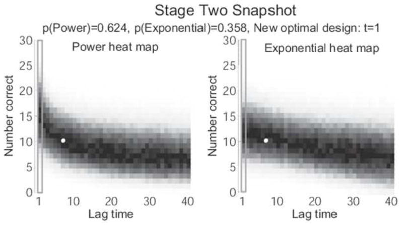
Another perspective on this first stage of the ADO experiment can be seen in Figures ?? and ??. In Figure ??, the optimal lag time lag time (t = 7) is highlighted with a blue rectangle on each of the heat maps. One indication as to why ADO identified this lag time as optimal for this stage is that t = 7 seems to be where the heat maps of the two models differ the most: the most likely number of correct responses according to the power model is between 10 and 15 while the most likely number of correct responses under the exponential model is between 20 and 25. When data were generated at t = 7, the result was 12 correct responses, which is more likely under the power model than under the exponential model. Accordingly, the posterior probability of the power model rises to 0.642, while the posterior probability of the exponential model drops to 0.358. These probabilities are shown in Figure ??, which gives a snapshot of the state of the experiment at the start of the second stage. The white dot in each of the heat maps in Figure ?? depicts the data point from the first stage, and the heat maps themselves show what ADO believes about the parameters of each model after updating on that data point. What’s notable is that both heat maps have converged around the observed data point. Importantly, however, this convergence changes both models’ predictions across the entire range of lag times. The updated heat maps no longer differ much at t = 7, but they now differ significantly at t = 1. Not coincidentally, ADO finds that t = 1 is the optimal lag time for the next stage of the experiment.

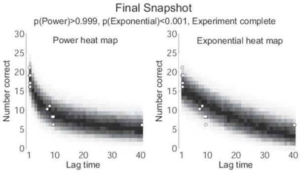
The simulation continued for ten ADO stages. In a real experiment, the experimenter could review a snapshot like Figure ?? after each stage in order to monitor the progress of the experiment. The experimenter could also add a human element to the design process by choosing a different design than that recommended by ADO for the next stage. For now, we will skip to a snapshot of the experiment after all ten stages have been completed. In Figure ??, the blue dots represent the ten data points that were observed, and the heat maps represent the best estimates of each model based on those ten data points. It is clear from the heat maps that the exponential model can not match the observed data pattern well, even at its best fitting parameters. On the other hand, the power model can fit the data perfectly (as it should, since it generated the data). Accordingly, the posterior probability of the power model is greater than 0.999, indicating that the data clearly identify it as the data generating model. Moreover, the heat map estimate of the power model closely resembles the heat map of the data-generating model in Figure ??, indicating that the parameters have converged to the correct values. Figure ?? shows a typical posterior model probability curve obtained from the ADO simulation experiment.

5 Limitations

While ADO has the potential to significantly improve the efficiency of data collection in psychological sciences, it is important that the reader is aware of the assumptions and limitation of the methodology. First of all, not all design variables in an experiment can be optimized in ADO. They must be quantifiable in such a way that the likelihood function depends explicitly on the values of the design variables being optimized (Myung and Pitt, 2009, p. 511). Consequently, ADO is not applicable to variables such as type of experimental task (word reading vs. lexical decision) and nominal variables (e.g., words vs. pictures). No statistical methodology currently exists that can handle such non-quantitative design variables.

Another limitation of the ADO methodology is the assumption that one of the models under consideration is the true, data-generating model. This assumption, obviously, is likely to be violated in practice, given that our models are merely imperfect representations of the real process under study.⁶ Ideally, one would like to optimize an experiment for an infinite array of models representing a whole spectrum of realities; no implementable methodology currently exists that can handle the problem of this scope.

The ADO algorithm is myopic in the sense that the optimization at each stage of experimentation is performed as if the current experiment is the last one to be conducted. In reality, however, the global optimality of the current designs depend upon the outcomes of future experiments, as well as those of the previous experiments. This sequential dependency of optimal designs is not considered in the present ADO algorithm, due to the huge computational resources needed to take into account the effect. Recent advances in approximate dynamic programming offers a potentially promising solution to overcome this challenge (e.g., Powell, 2007).

Perhaps the most challenging problem is extending the ADO framework to a class of simulation-based models (e.g., Reder et al., 2000; Polyn et al., 2009) that are defined in terms of a series of steps to be simulated on computer without explicit forms of likelihood functions –a prerequisite to implement the current ADO algorithm. Given the popularity of these types of models in cognitive science, ADO will need to be expanded to accommodate them, perhaps using a likelihood-free inference scheme known as Approximate Bayesian Computation (e.g., Beaumont et al., 2009; Turner and Van Zandt, 2012).

6 Conclusions

In this article, we provided a tutorial exposition of adaptive design optimization (ADO). ADO allows users to intelligently choose experimental stimuli on each trial of an experiment in order to maximize the expected information gain provided by each outcome. We began the tutorial by contrasting ADO against the traditional, non-adaptive heuristic approach to experimental design, then presented the nuts and bolts of the practical implementation of ADO, and finally, illustrated an application of the experimental technique in simulated experiments to discriminate between two retention models.

Use of ADO requires becoming comfortable with a different style of experimentation. Although the end goal, whether it be parameter estimation or model discrimination, is the same as traditional methods, how you get there differs. The traditional method is a group approach that emphasizes seeing through individual differences to capture the underlying regularities in behavior. This is achieved by ensuring stable performance (parameters) through random and repeated presentation of stimuli and testing sufficient participants (statistical power). Data analysis compares the strength of the regularity against the amount of noise contributed by participants. There is no escaping individual variability, so ADO exploits it by presenting a stimulus whose information value is likely to be greatest for that given participant and trial, as determined by optimization of an objective function. This means that each participant will likely receive a different subset of the stimuli. In this regard, the price of using ADO is some loss of control over the experiment; the researcher turns over stimulus selection to the algorithm, and places faith in it to achieve the desired ends. The benefit is a level of efficiency that cannot be achieved without the algorithm. In the end, it is the research question that should drive choice of methodology. ADO has many uses, but at this point in its evolution, it would be premature to claim it is always superior.

In conclusion, the advancement of science depends upon accurate inference. ADO, though still in its infancy, is an exciting new tool that holds considerable promise in improving inference. By combining the predictive precision of the computational models themselves and the power of state of the art statistical computing techniques, ADO can make experimentation informative and efficient, thereby making the tool attractive on multiple fronts. ADO takes full advantage of the design space of an experiment by probing repeatedly, in each stage, those locations (i.e., designs) that should be maximally informative about the model(s) under consideration. In time-sensitive and resource-intensive situations, ADO’s efficiency can reduce the cost of equipment and personnel. This potent combination of informativeness and efficiency in experimentation should accelerate scientific discovery in cognitive science and beyond.

Figure 1.

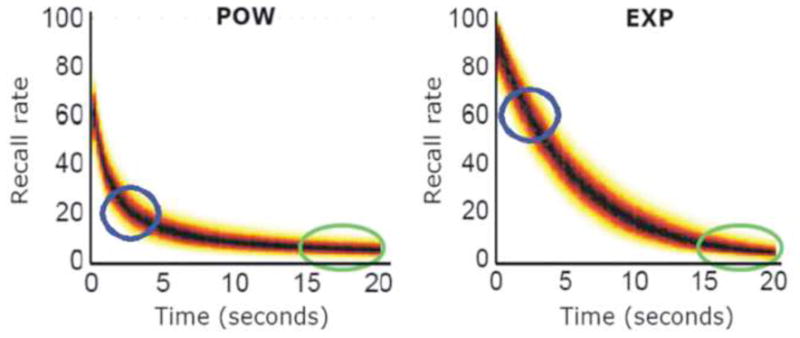
Sample power (POW) and exponential (EXP) functions, generated from a narrow range of model parameters (see text). The time intervals between 1 and 5 seconds, where the models are the most discriminable, are indicated by the blue circles. In contrast, the green elliptic circles indicate the time intervals (i.e., 15 – 20 seconds) that offer the least discriminability.

Figure 2.

Schematic illustration of the traditional experimentation versus adaptive experimentation paradigm. (a) The vertical arrow on the left represents optimization of the values of design variables before data collection. The vertical arrow on the right represents the analysis and modeling of the data collected, using model selection or parameter estimation methods, for example. (b) In the adaptive experimentation paradigm, the three parts of experimentation (design optimization, experiment, and data modeling) are closely integrated to form a cycle of inference steps in which the output from one part is fed as an input to the next part.

Figure 4.

The grid search algorithm.

Figure 5.

Illustration of sequential Monte Carlo search design optimization with simulated annealing.

Figure 6.

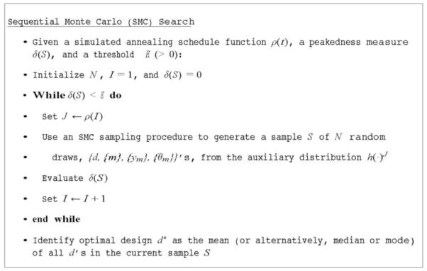
The SMC search algorithm.

Figure 8.

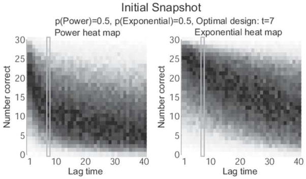
Heat maps of the Power model (left) and Exponential model (right) representing ADO’s prior estimates of each model. Darker colors indicate regions of higher probability. The lag time of t = 7 (blue rectangle) is chosen for testing in the first stage because it is the place where the two models differ the most, based on the priors.

Figure 9.

Heat maps of the Power model (left) and Exponential model (right) representing ADO’s estimates of each model after the first stage of testing (prior to the second stage). Estimates have converged around the observed data point (white dot in each heat map). ADO selects t = 1 (blue rectangle) for testing in Stage 2 because it is the place where the two models differ the most, based on these updated estimates.

Figure 10.

Heat maps of the Power model (left) and Exponential model (right) representing ADO’s estimates of each model after the ten stages of testing. Both models try to fit the observed data points (white dots) as well as possible, but the exponential model cannot do so as well as the power model. The difference is so extreme that the power model is over 1000 times more likely to generate this pattern of data than the exponential model.

Figure 11.

Posterior model probability curve from a sample run of the ADO simulation experiment. The data were generated from the power model with parameters a = 0.80 and b = 0.40. See the text for additional details of the simulation.

Highlights.

• Introduces the reader to adaptive design optimization (ADO)

• ADO is a Bayesian framework for optimizing experimental designs

• Provides the conceptual, theoretical, and computational foundations of ADO

• Serves as practical guide to applying ADO to simple cognitive models.

References

- Akaike H. Information theory and an extension of the maximum likelihood principle. In: Petrov BN, Caski F, editors. Proceedings of the Second International Symposium on Information Theory. Budapest: Akademiai Kiado; 1973. pp. 267–281. [Google Scholar]
- Amzal B, Bois F, Parent E, Robert C. Bayesian-optimal design via interacting particle systems. Journal of the American Statistical Association. 2006;101(474):773–785. [Google Scholar]
- Andrieu C, DeFreitas N, Doucet A, Jornan MJ. An introduction to MCMC for machine learning. Machine Learning. 2003;50:5–43. [Google Scholar]
- Atkinson A, Donev A. Optimum Experimental Designs. Oxford University Press; 1992. [Google Scholar]
- Atkinson A, Federov V. Optimal design: Experiments for discriminating between several models. Biometrika. 1975;62(2):289. [Google Scholar]
- Beaumont MA, Cornuet JM, Marin JM, Robert CP. Adaptive approximate Bayesian computation. Biometrika. 2009;52:1–8. [Google Scholar]
- Bellman RE. Dynamic Programming (reprint edition) Dover Publications; Mineola, NY: 2003. [Google Scholar]
- Berry DA. Bayesian clinical trials. Nature Reviews. 2006;5:27–36. doi: 10.1038/nrd1927. [DOI] [PubMed] [Google Scholar]
- Bölte A, Thonemann UW. Optimizing simulated annealing schedule with genertic programming. European Journal of Operational Research. 1996;92:402–416. [Google Scholar]
- Box G, Hill W. Discrimination among mechanistic models. Technometrics. 1967;9:57–71. [Google Scholar]
- Burnham KP, Anderson DR. Model Selection and Multi-Model Inference: A Practical Information-Theoretic Approach. 2. Springer; New York, NY: 2010. [Google Scholar]
- Carlin HP, Louis TA. Bayes and empirical Bayes methods for data analysis. 2. Chapman & Hall; 2000. [Google Scholar]
- Cavagnaro D, Gonzalez R, Myung J, Pitt M. Optimal decision stimuli for risky choice experiments: An adaptive approach. Management Science. 2013a;59(2):358–375. doi: 10.1287/mnsc.1120.1558. [DOI] [PMC free article] [PubMed] [Google Scholar]
- Cavagnaro D, Pitt M, Gonzalez R, Myung J. Discriminating among probability weighting functions using adaptive design optimization. Journal of Risk and Uncertainty. 2013b doi: 10.1007/s11166-013-9179-3. in press. [DOI] [PMC free article] [PubMed] [Google Scholar]
- Cavagnaro D, Pitt M, Myung J. Model discrimination through adaptive experimentation. Psychonomic Bulletin & Review. 2011;18(1):204–210. doi: 10.3758/s13423-010-0030-4. [DOI] [PMC free article] [PubMed] [Google Scholar]
- Cavagnaro DR, Myung JI, Pitt MA, Kujala JV. Adaptive design optimization: A mutual information based approach to model discrimination in cognitive science. Neural Computation. 2010;22(4):887–905. doi: 10.1162/neco.2009.02-09-959. [DOI] [PubMed] [Google Scholar]
- Cavagnaro DR, Pitt MA, Myung JI. Adaptive design optimization in experiments with people. Advances in Neural Information Processing Systems. 2009;22:234–242. [Google Scholar]
- Chaloner K, Verdinelli I. Bayesian experimental design: A review. Statistical Science. 1995;10(3):273–304. [Google Scholar]
- Cobo-Lewis AB. An adaptive psychophysical method for subject classification. Perception & Psychophysics. 1997;59:989–1003. doi: 10.3758/bf03205515. [DOI] [PubMed] [Google Scholar]
- Cohn D, Atlas L, Ladner R. Improving generalization with active learning. Machine Learning. 1994;15(2):201–221. [Google Scholar]
- Cohn D, Ghahramani Z, Jordan M. Active learning with statistical models. Journal of Artificial Intelligence Research. 1996;4:129–145. [Google Scholar]
- Cover T, Thomas J. Elements of Information Theory. John Wiley & Sons, Inc; 1991. [Google Scholar]
- Doucet A, de Freitas N, Gordon N. Sequential Monte Carlo Methods in Practice. Springer; 2001. [Google Scholar]
- Gelman A, Carlin J, Stern H, Rubin D. Bayesian Data Analysis. Chapman & Hall; 2004. [Google Scholar]
- Gill J. Bayesian Methods: A Social and Behavioral Sciences. 2. Chapman and Hall/CRC; New York, NY: 2007. [Google Scholar]
- Grünwald PD. A tutorial introduction to the minimum description length principle. In: Grünwald P, Myung IJ, Pitt MA, editors. Advances in Minimum Description Length: Theory and Applications. The M.I.T. Press; 2005. [Google Scholar]
- Hambleton RK, Swaminathan H, Rogers HJ. Fundamentals of Item Response Theory. Sage Publications; Newbury Park, CA: 1991. [Google Scholar]
- Jeffreys H. Theory of Probability. Oxford University Press; Oxford, UK: 1961. [Google Scholar]
- Kass RE, Raftery AE. Bayes factors. Journal of the American Statistical Association. 1995;90:773–795. [Google Scholar]
- Kass RE, Wasserman L. The selection of prior distributions by formal rules. Journal of the American Statistical Association. 1996;91(435):1343–1370. [Google Scholar]
- Kirkpatrick S, Gelatt C, Vecchi M. Optimization by simulated annealing. Science. 1983;220:671–680. doi: 10.1126/science.220.4598.671. [DOI] [PubMed] [Google Scholar]
- Kontsevich LL, Tyler CW. Bayesian daptive estimation of psychometric slope and threshold. Vision Research. 1999;39:2729–2737. doi: 10.1016/s0042-6989(98)00285-5. [DOI] [PubMed] [Google Scholar]
- Kreutz C, Timmer J. Systems biology: Experimental design. FEBS Journal. 2009;276:923–942. doi: 10.1111/j.1742-4658.2008.06843.x. [DOI] [PubMed] [Google Scholar]
- Kruschke JK. Doing Bayesian Data Analysis: A Tutorial with R and BUGS. AcademiC Press; New York, NY: 2010. [Google Scholar]
- Kujala J, Lukka T. Bayesian adaptive estimation: The next dimension. Journal of Mathematical Psychology. 2006;50(4):369–389. [Google Scholar]
- Lesmes L, Jeon ST, Lu ZL, Dosher B. Bayesian adaptive estimation of threshold versus contrast external noise functions: The quick T vC method. Vision Research. 2006;46:3160–3176. doi: 10.1016/j.visres.2006.04.022. [DOI] [PubMed] [Google Scholar]
- Lesmes L, Lu ZL, Baek J, Dosher B. Bayesian adaptive estimation of the contrast sensitivity function: The quick SCF method. Journal of Vision. 2010;10:1–21. doi: 10.1167/10.3.17. [DOI] [PMC free article] [PubMed] [Google Scholar]
- Lewi J, Butera R, Paninski L. Sequential optimal design of neurophysiology experiments. Neural Computation. 2009;21:619–687. doi: 10.1162/neco.2008.08-07-594. [DOI] [PubMed] [Google Scholar]
- Lindley D. On a measure of the information provided by an experiment. Annals of Mathematical Statistics. 1956;27(4):986–1005. [Google Scholar]
- Loredo TJ. Bayesian adaptive exploration. In: Erickson GJ, Zhai Y, editors. Bayesian Inference and Maximum Entropy Methods in Science and Engineering: 23rd International Workshop on Bayesian Inference and Maximum Entropy Methods in Science and Engineering. Vol. 707. American Institute of Physics; 2004. pp. 330–346. [Google Scholar]
- Müller P. Simulation-based optimal design. In: Berger JO, Dawid AP, Smith AFM, editors. Bayesian Statistics. Vol. 6. Oxford, UK: Oxford University Press; 1999. pp. 459–474. [Google Scholar]
- Müller P, Sanso B, De Iorio M. Optimal Bayesian design by inhomogeneous Markov chain simulation. Journal of the American Statistical Association. 2004;99(467):788–798. [Google Scholar]
- Myung JI, Pitt MA. Optimal experimental design for model discrimination. Psychological Review. 2009;58:499–518. doi: 10.1037/a0016104. [DOI] [PMC free article] [PubMed] [Google Scholar]
- Nelson J. Finding useful questions: On Bayesian diagnosticity, probability, impact, and information gain. Psychological Review. 2005;112(4):979–999. doi: 10.1037/0033-295X.112.4.979. [DOI] [PubMed] [Google Scholar]
- Nelson J, McKenzie CRM, Cottrell GW, Sejnowski TJ. Experience matters: Information acquisition optimizes probability gain. Psychological Science. 2011;21(7):960–969. doi: 10.1177/0956797610372637. [DOI] [PMC free article] [PubMed] [Google Scholar]
- Oberauer K, Lewandowsky S. Forgetting in immediate serial recall: Decay, temporal distinctiveness, or interference? Psychological Review. 2008;115(3):544–576. doi: 10.1037/0033-295X.115.3.544. [DOI] [PubMed] [Google Scholar]
- Pitt MA, Myung IJ, Zhang S. Toward a method of selecting among computational models of cognition. Psychological Review. 2002;190(3):472–491. doi: 10.1037/0033-295x.109.3.472. [DOI] [PubMed] [Google Scholar]
- Polyn SM, Norman KA, Kahana MJ. A context maintenance and retrieval model of organizational processes in free recall. Psychological Review. 2009;116:129–156. doi: 10.1037/a0014420. [DOI] [PMC free article] [PubMed] [Google Scholar]
- Powell WB. Approximate Dynamic Programming: Solving the Curses of Dimensionality. John Wiley & Sons; Hoboken, New Jersey: 2007. [Google Scholar]
- Reder LM, Nhouyvanisvong A, Schunn CD, Avyers MS, Angstadt P, Hiraki K. A mechanistic account of the mirror effect for word frequency: A computational model of remember-know judgments in a continuous recognition paradigm. Journal of Experimental Psychology: Learning, Memory and Cognition. 2000;26:294–320. doi: 10.1037//0278-7393.26.2.294. [DOI] [PubMed] [Google Scholar]
- Rissanen J. Modeling by shortest data description. Automatica. 1978;14:461–471. [Google Scholar]
- Robert CP. The Bayesian Choice: From Decision-Theoretic Foundations to Computational Implementation. 2. Springer; New York, NY: 2001. [Google Scholar]
- Robert CP, Casella G. Monte Carlo Statistical Methods. 2. Springer; New York, NY: 2004. [Google Scholar]
- Rubin D, Wenzel A. One hundred years of forgetting: A quantitative description of retention. Psychological Review. 1996;103(4):734–760. [Google Scholar]
- Sutton RS, Barto AG. Reinforcement Learning: An Introduction. MIT Press; Cambridge, Massachusetts: 1998. [Google Scholar]
- Tang Y, Young C, Myung JI, Pitt MA, Opfer J. Optimal inference and feedback for representational change. In: Ohlsson S, Catrambone R, editors. Proceedings of the 32nd Annual Meeting of the Cognitive Science Society. Austin, TX: Cognitive Science Society; 2010. pp. 2572–2577. [Google Scholar]
- Turner B, Van Zandt T. A tutorial on approximate bayesian computation. Journal of Mathematical Psychology. 2012;56(2):69–85. [Google Scholar]
- van der Linden WJ, Glas CAW. Computerized Adaptive Testing. Kluwer Academic Publishers; Boston, MA: 2000. [Google Scholar]
- van Erven T, Grünwald PD, de Rooji S. Catching up faster by switching sooner: A predictive approach to adaptive estimation with an application to the AIC-BIC Dilemma. Journal of the Royal Statistical Society, Series B. 2012;74:361–397. [Google Scholar]
- Vul E, Bergsma J, MacLeod IA. Functional adaptive sequential testing. Seeing and Perceiving. 2010;23:483–513. doi: 10.1163/187847510x532694. [DOI] [PubMed] [Google Scholar]
- Wagenmakers EJ, Grünwald PD, Steyvers M. Accumulative prediction error and the selection of time series models. Journal of Mathematical Psychology. 2006;50:149–166. [Google Scholar]
- Wathen JK, Thall PF. Bayesian adaptive model selection for optimizing group sequential clinical trials. Statistics in Medicine. 2008;27:5586–5604. doi: 10.1002/sim.3381. [DOI] [PMC free article] [PubMed] [Google Scholar]
- Weiss DJ, Kingsbury GG. Application of computerized adaptive testing to educational problems. Journal of Educational Measurement. 1984;21:361–375. [Google Scholar]
- Wixted J, Ebbesen E. On the form of forgetting. Psychological Science. 1991;2(6):409–415. [Google Scholar]