Abstract
We describe here the PRIMO (PRotein Intermediate Model) force field, a physics-based fully transferable additive coarse-grained potential energy function that is compatible with an all-atom force field for multi-scale simulations. The energy function consists of standard molecular dynamics energy terms plus a hydrogen-bonding potential term and is mainly parameterized based on the CHARMM22/CMAP force field in a bottom-up fashion. The solvent is treated implicitly via the generalized Born model. The bonded interactions are either harmonic or distance-based spline interpolated potentials. These potentials are defined on the basis of all-atom molecular dynamics (MD) simulations of dipeptides with the CHARMM22/CMAP force field. The non-bonded parameters are tuned by matching conformational free energies of diverse set of conformations with that of CHARMM all-atom results. PRIMO is designed to provide a correct description of conformational distribution of the backbone (ϕ/ψ) and side chains (χ1) for all amino acids with a CMAP correction term. The CMAP potential in PRIMO is optimized based on the new CHARMM C36 CMAP. The resulting optimized force field has been applied in MD simulations of several proteins of 36–155 amino acids and shown that the root-mean-squared-deviation of the average structure from the corresponding crystallographic structure varies between 1.80 and 4.03 Å. PRIMO is shown to fold several small peptides to their native-like structures from extended conformations. These results suggest the applicability of the PRIMO force field in the study of protein structures in aqueous solution, structure predictions as well as ab initio folding of small peptides.
Keywords: Coarse-grain, force field, implicit solvent, molecular dynamics, replica exchange
1. Introduction
Computer simulations are indispensable tools in the study of biomolecular systems, complementing experiments. The latest generation of atomistic force fields combined with powerful computing platforms and/or efficient enhanced sampling and methodologies are resulting in increasingly realistic descriptions of biomolecular dynamics. Most notables are recent folding studies of small proteins that would have been unthinkable not long ago1,2. However, although such studies are impressive, atomistic simulations are still several magnitudes away from being able to effectively cover both, the spatial and temporal scales of cellular processes. One solution to this problem is the simplification of the model that is used to describe the biological system. This is typically accomplished by coarse-graining (CG) to represent a given system with a reduced number of degrees of freedom vs. a complete all-atom description. The reduction in the degrees of freedom in CG models translates immediately into less computational demands and offers additional benefits by allowing longer integration time steps in molecular dynamics (MD) simulations, for example, and generating accelerated dynamics due to smoother energy landscapes. As a result, CG models may be able to cover dramatically longer simulation times and length scales compared to fully atomistic models.
Many CG models of varying complexity have been proposed for proteins3–7 since the pioneering work of Levitt and Warshel8. At the beginning, most of these models were developed with specific applications, such as study of structural features of viral capsid9, structure and dynamics protein membrane systems10, protein structure prediction11,12, scoring protein decoys13,14, protein-protein docking15, and protein folding studies16–20 in mind. The resolution of CG models may range from one or a few particles per protein15–20 to near atomistic resolutions11,21,22. A popular CG representation involves one interaction site per amino acid residue, usually located on the Cα atom23. At such a resolution, detailed properties of specific proteins are difficult to capture, but such models are well-suited for studying the kinetics and overall mechanisms of protein folding processes20,24. Most of these models are highly system-specific, such as widely used Go models23, but there are also examples of semi-transferable models with limited accuracy12. Recent examples of such models include the following: Tozzini and McCammon25 have developed a coarse-grained model to study the dynamics of flap opening in HIV-1 protease. In their model, each amino acid is represented by a single bead placed on the Cα atom. The force field was parameterized based on the Boltzmann inversion procedure. On the other hand, Brini and van der Vegt proposed a free-energy-based coarse-graining procedure, namely conditional reversible work (CRW)26. Here, the coarse-graining is performed at the pair level, and is used to describe the interaction free energy between two mapped atom groups (beads) embedded in their respective chemical environment. CRW-CG potentials are ideally suited for studies of chemical transferability. In order to study the disordered state of proteins, Ghavami and co-workers27 have proposed a one-bead-per-amino-acid model. In this model, residue and sequence specific bending and torsion potentials for the bonded interactions are extracted from Ramachandran data of the coil regions of proteins in the Protein Data Bank. This model has been used successfully to predict the scaling relations of denatured proteins. However, in the absence of electrostatic and hydrophobic interactions in their model, one cannot study natively unfolded proteins under physiological conditions.
Higher resolution CG models typically involve a few interaction sites for representing the backbone plus additional sites for the side chains. Such models are used for a broader set of applications, including mechanistic studies and for protein structure prediction11,12,19. These higher-resolution models have a greater potential for transferability between different systems and different environments. The transferability of CG models becomes more likely with generally applicable, usually physics-based potentials vs. empirical, system-specific terms. A common recipe used in such models involves two steps: (i) the calculation of thermodynamic, structural properties of a reference system from an atomistic simulation, and (ii) fitting of the parameters in suitable potentials to match these properties. Recently, many such models have been proposed and the most prominent models in this are described briefly in the following: In the UNRES model18,28, a polypeptide chain is represented as a sequence of α-carbon atoms with attached united side chains and united peptide groups, each of the latter being positioned in the middle between two consecutive Cα atoms. The potential function of UNRES is parameterized against free energies from atomistic polypeptide simulations in explicit water using a functional form that resembles atomistic force fields but with additional terms. Although UNRES mostly relies on physical terms, UNRES also contains interaction potentials that are derived from a statistical analysis of structures in the Protein Data Bank (PDB). With UNRES, solvent effects are represented implicitly. Applications of UNRES to date have been largely limited to de novo protein folding16 and structure prediction29.
In the MARTINI30–33 model, four heavy atoms are represented on average by a single interaction center. Ring-like molecules are an exception and mapped at higher resolution (up to two-to-one). The model considers four main types of interaction sites: polar (P), nonpolar (N), apolar (C) and charged (Q). The MARTINI model is parameterized by matching the thermodynamic partitioning free energy of amino acid side chains between the polar and hydrophobic phases similar to how the recent version of the GROMOS force field was developed34. The MARTINI model is too coarse-grained to be able to accurate reflect amino-acid specific secondary structure propensities. Therefore, a weak bias has to be added to maintain secondary structures according to what is known from native structures. In the MARTINI model, solvent effects are modeled explicitly with coarse-grained water or lipid molecules. While this increases the computational complexity over other CG models, it provides transferability between water and membrane phases. Consequently, the majority of applications of the MARTINI force field involves membrane-interacting biomolecules, in particular studies of the self-assembly of transmembrane proteins30 and gating mechanisms in mechanically-gated32 and voltaged-gated33 membrane ion channels.
The OPEP11,35 (Optimized Potential for Efficient structure Prediction) model is based on a six-bead model per amino acid where the backbone is modeled in atomistic detail (without hydrogens) while a single centroid bead represents side chains. The implicit solvent OPEP function is expressed as a sum of short-range (bond lengths, bond angles, improper torsions of the side chains and the amide bonds, backbone torsions), van der Waals, and two-body as well as four-body hydrogen-bonding interactions. The potential function was parameterized with the main goal of finding the lowest free energy for native structures relative to non-native decoys. The OPEP force field has been used primarily to study protein stabilities and the folding of small peptides36 but also to the oligomerization of amyloid peptide37 and the fast structure prediction of miniproteins38,39.
Another CG model that describes the side chain as a single interaction center was developed by Irbäck and coworkers21,22. Each residue retains the backbone atoms Cα, C, and N as well as the O and H of the backbone units. The side chain is represented by a Cβ only and can be hydrophobic, hydrophilic, or absent (glycine). Bond lengths and bond angles are kept fixed so that the internal coordinates reduce to the backbone dihedral ϕ and ψ. The energy function of this model is simply given by the sum of a dihedral term, an excluded-volume term, a hydrogen-bonding energy, and a potential of interaction between hydrophobic residues. Because this model was parameterized empirically to reproduce the features of a specific set of proteins under investigation, its application to other proteins may require a re-adjustment of the parameters.
The Hall group has developed a four-bead (three backbone beads-N, Cα, C′ and one minimalist side chain bead Cβ) coarse-grained model, PRIME40,41 that was used in protein aggregation. Instead of traditional molecular dynamics, PRIME uses discrete molecular dynamics (DMD), which is applicable to discontinuous potentials such as the hard-sphere and square-well potentials. The parameters were obtained by applying a perceptron-learning algorithm and a modified stochastic learning algorithm that optimizes the energy gap between 711 knows native states from the PDB and decoy structures generated by gapless threading. Later, Ding et al.42 extended this model by adding one or two more additional effective side-chain atoms. For the β-branched amino acids (Thr, Ile, and Val), two γ-beads representing the two branches after Cβ were introduced while an additional δ-bead was introduced for bulky amino acids (Arg, Lys, and Trp).
The multi-scale coarse-graining (MS-CG) method43,44 takes a somewhat different approach by not relying on a pre-defined potential. Instead, atomistic force information from reference simulations is utilized within a variational framework to systematically develop CG models from the bottom-up for a particular biomolecular system of interest. The MS-CG approach can be applied at various resolutions. In principle, the resulting MS-CG potential will be an accurate representation of the optimal CG potential provided that the basis set for the variational calculation is complete enough and that the canonical distribution of atomistic sites is well sampled by the data set45,46. The MS-CG method has been applied to the study of protein folding and dynamics17,43. However, the level of coarse-graining prevents the accurate conversion of CG models to atomistic resolution. In addition, the resulting MS-CG potentials commonly suffer from a lack of transferability.
Other recent CG models include a model by Bereau and Deserno47 for protein folding and aggregation involves an intermediate representation with four beads per amino acid and implicit solvent treatment and the PaLaCe (Pasi-Lavery-Ceres) model proposed by Pasi and co-workers48. The PaLaCe model has been parameterized using Boltzmann inversion of conformational probability distribution derived from a protein structure data set, and iteratively refined to reproduce the experimental distribution. PaLaCe uses a two-tier representation with one to three pseudo-atoms representing each amino acid for the non-bonded interactions, combined with an atomic-scale peptide backbone48. The PaLaCe model has been used for energy minimization, normal mode calculations, and molecular or stochastic dynamics.
A recent trend has been to develop hybrid models where part of a system is represented in atomistic detail while other parts are represented at the CG level. Recently, Zacharias49 has developed a hybrid united atom/coarse-grained model for proteins where the interactions of protein main chain sites are based on the GROMOS united atom force field. However, non-bonded interactions between side chains and between side chains and main chain sites are calculated at the level of a CG model using the knowledge-based ATTRACT potential50. Rzepiela and co-workers51 have proposed such a mixed model between all-atom and MARTINI CG force fields where all-atom-CG interactions are replaced by CG interactions through dummy sites. This avoids the need for re-parameterization of cross-resolution terms from the CG perspective but it does not fully address the environment seen by the atomistic part.
In a similar effort, the Schulten group52 has developed PACE (Protein in Atomistic details coupled with Coarse-grained Environment) where a united-atom protein model is coupled with MARTINI CG water and/or MARTINI CG lipids. In PACE, cross-resolution parameters were optimized through the reproduction of experimental thermodynamic quantities. Moreover, in the context of the hybrid force field, the interactions of atomic sites in proteins were reparameterized by using different reference data, such as potentials of mean force (PMF) of polar interactions from atomistic simulations and statistical backbone potentials from a Protein Data Bank (PDB) coil library52. Atomistic partial charges from all-atom force fields were then combined with PACE to provide a more realistic description of interactions between charged groups. PACE has been successfully used to fold a series of peptides and proteins, but challenges remain in accurately estimating the stabilities of native structures53.
Although, there are many CG models now available, transferability between different systems and to different environments as well as an ability to combine with atomistic force fields in hybrid AA/CG multi-scale approaches remains a challenge that has not been fully addressed. We are here proposing a new CG model, PRIMO (Protein Intermediate Model) which aims to improve transferability and is meant to be more compatible with atomistic levels of detail. A key feature of PRIMO is a somewhat higher resolution that was chosen such that fast and accurate reconstruction to all-atom representations becomes possible. This model and the reconstruction procedure have been described previously54,55. Although PRIMO reduces the number of interactions three-to four folds over fully atomistic models, all-atom models can be reconstructed at negligible computational cost to accuracies of 0.1 Å54. This feature is unique among CG models proposed so far and is the basis for tight integration with atomistic force fields. Furthermore, the PRIMO force field can be energetically matched to atomistic force fields with the benefits of greater transferability and better suitability for AA/CG approaches.
In this paper, the force field for PRIMO is presented. The PRIMO energy function consists of standard molecular dynamics energy terms plus a hydrogen-bonding potential term. We followed a bottom-up approach similar to those used in the development of classical all-atom force fields as well as other coarse-grained fore fields, such as MARTINI, UNRES, and PaLaCe to design the PRIMO force field. One of the advantages of a bottom-up approach is a modular design of the potential energy function. This allows the breakdown of the overall interactions into simple physics-based energy functions that were parameterized separately. In the development of PRIMO, the basic biological building blocks, such as amino acids, were rigorously parameterized and validated to form the basis for transferability of the resulting model to any arbitrary protein system. A key feature is the use of a physical implicit solvent model to maintain transferability to different environments. The PRIMO force field is primarily parameterized based on the CHARMM22/CMAP56,57 force field with adjustments to incorporate recent updates to the CHARMM force field58,59. The resulting PRIMO force field targets a wide range of applications ranging from structure prediction and ab initio folding to mechanistic studies of protein dynamics, in particular in the context of AA/CG modeling schemes.
The remainder of this article is organized into the following sections: First, we briefly review the PRIMO CG model and introduce its energy function. Next, the PRIMO force field parameterization procedure is described. Then, we describe the validation of the force field by comparing the stability and structural properties of several proteins with those of all-atom simulations. Finally, we discuss the conformational sampling of alanine-based polypeptides and folding studies of small peptides with diverse structural motifs.
2. PRIMO Mapping
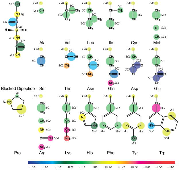
The PRIMO model, i.e. its mapping from atomistic to coarse-grained sites was described previously54,55. It is only briefly reviewed here. The CG sites were chosen in such a way that an analytical reconstruction of all-atom representations from CG models based on molecular bonding geometries is possible. The CG interaction sites for amino acids are illustrated in Figure 1. Table S1 (see Supporting Information) lists the mapping between all-atom and PRIMO CG levels. The backbone is represented with N, Cα, and a combined carbonyl site (CO) placed at the geometric center of the carbonyl C and O atoms. This ensures the preservation of backbone hydrogen bonding interactions, which is essential for an accurate description of the secondary structures of a protein. Non-glycine side chains are represented with one to five CG sites (referred to as SCn, where n is the index of the CG side chain site). The amino acids Ala, Cys, Pro, Ser, and Val have only one SC1 particle; the amino acids Ile, Leu, and Thr are modeled with SC1 and SC2 sites; the amino acids Asn, Asp, Gln, Glu, His, Met, and Phe are described by three SC sites; the amino acids Lys, Trp, and Tyr consist of four SC particles; the Arg side chain possesses five SC interaction sites. A typical representation of an all-atom protein in PRIMO is shown in Figure S1.
Figure 1.
PRIMO model for amino acids. The size of the spheres indicates van der Waals radii. Colors indicate charges according to color bar given at the bottom.
In this work, the following convention is followed to refer to the CG, atomistic or virtual particles: (i) an upper case alpha-numeric name for CG (e.g., CA1, N1 etc.); (ii) a lower case combination of alpha-numeric and Greek symbol for all-atom sites (e.g., cα, cδ1 etc.); and (iii) virtual atoms are represented like all-atom sites, but with a superscript * (e.g., cβ*, cγ*, cδ1*).
3. PRIMO Energy Function
The PRIMO interaction potential consists of a standard molecular dynamics force field-like form with additional spline-based bonded terms to maintain correct bond geometries at the coarse-grained level, an explicit H-bonding potential, and a combined generalized Born (GB)/atomic solvation parameters (ASP) implicit solvent model. The details of the PRIMO energy function are described below.
3.1 Bonded Interactions
| (1) |
Bonded interactions between PRIMO sites represent both, real covalent bonds, such as between Cα and N backbone sites, and virtual bonds, such as between N and the combined backbone carbonyl site CO. The real covalent bonds such as 1–2 (bonds) and 1–3 (angles) interactions are generally described by standard harmonic potentials. Virtual bonds are described primarily with distance-based spline-interpolated potentials in order to capture non-harmonic potential shapes and the presence of multiple minima (see Eq. 2 and 3).
| (2) |
| (3) |
For some side chains, these terms were not found to be sufficient to maintain stereochemically correct geometries. In those cases, the primary PRIMO interaction sites were augmented by virtual atomic sites that are reconstructed on-the-fly from the PRIMO sites, thus avoiding additional degrees of freedom. Additional bonded interactions were then introduced between the virtual sites and the primary PRIMO interaction sites (see Eq. 4 and 5).
| (4) |
| (5) |
The computational impact of adding virtual atoms is minimal because the reconstruction is very fast and involves only a few sites. Furthermore, a multiple time step scheme where virtual sites are not reconstructed at every step is possible. It should also be stressed, that the role of the virtual sites is only to improve local molecular geometries through bonded interactions and that these sites do not participate in the calculation of non-bonded interactions, which is by far the most time consuming component of the PRIMO force field.
To further illustrate how virtual atoms are being used, Figure S2 shows the treatment of phenylalanine as an example. For this residue, the primary CG sites are located at cε1 (SC2), cε2 (SC3), and at the midpoint between cβ and cγ (SC1). Based on stereochemistry, the sampling of the SC1 particle should be restricted to a circle around the cα-cβ bond because of sp3-hybridization of bonds to cβ. However, the angle terms such as N1-CA1-SC1, CO-CA1-SC1, and other bonded terms are insufficient to maintain the SC1 particle on such a circle. As a result, the PRIMO model would result in non-chemical structures when reconstructed to all-atom detail. An additional issue with phenylalanine is the planarity of the aromatic ring that is not maintained with just the three primary PRIMO sites. To alleviate the issue, two virtual atoms, cβ* and cγ*, are introduced that are reconstructed on-the-fly. The virtual atom cβ* is reconstructed using the “scheme 1” protocol described previously and the cγ* atom is reconstructed based on “scheme 2” protocol, as discussed in our previous papers47,48. Using the virtual sites, weak harmonic potentials involving CA1-cβ*-SC1, cγ*-SC2, and cγ*-SC3 interactions are then added to the existing potential with the result that the sampling of the SC1, SC2, and SC3 sites is restricted to positions consistent with the correct stereochemical geometries when reconstructed to full atomistic detail. Because the bonded terms between PRIMO sites were parameterized based on potentials of mean force (PMFs) from explicit solvent simulations (see below), there is a concern that the additional bonded interactions to virtual sites may distort the energy function. This is discussed in more detail in the next section. A list of all virtual sites, their reconstruction, and which bonded interactions they are involved in is given in Table S2 in the Supporting Information.
In all-atom force fields, 1–4 interactions are typically modeled as a combination of Fourier-series torsional terms and scaled electrostatic and Lennard–Jones interactions. In PRIMO, the 1–4 interactions are modeled as a combination of Fourier series torsional terms (Etorsion), distance-based spline-interpolated functions (Espline1–4), and a reduced Lennard–Jones (LJ) potential (ELJ1–4) in order to avoid hard-sphere overlap. A 1–4 electrostatic term is not included in PRIMO because the reduced charges used for PRIMO sites (see below) do not provide sufficiently accurate local electrostatic interactions. Instead the spline-based 1–4 interaction potentials are employed in our model to represent effective interactions in explicit solvent that are extracted from the dipeptide simulations. The functional forms of these terms are shown in Eq. 6–8.
| (6) |
| (7) |
| (8) |
In addition to the one-dimensional 1–4 terms, a spline-interpolated two-dimensional cross-correlation term (ECMAP) based on the CMAP methodology60 is used in PRIMO to couple the sampling of CO–N–CA–CO and N–CA–CO–N torsions. The advantage of using the CMAP methodology is that it is possible to nearly exactly reproduce any given target ϕ/ψ-map as demonstrated in the development of the atomistic CHARMM force fields60. The general functional form is given in Eq. 9. In PRIMO, it is used for the backbone torsion angles calculated from the PRIMO sites – which differ slightly from the torsion angles at the atomistic level.
| (9) |
3.2 Non-bonded Interactions
Non-bonded (Enb) terms in PRIMO consist of standard LJ terms (ELJ), Coulombic electrostatic interactions (Eelec), and an explicit angle-and distance-dependent hydrogen bonding potential (EHBOND) (see Eq. 10)
| (10) |
The van der Waals interaction between CG particles is described by the Lennard-Jones potential energy function according to Eq. 11
| (11) |
where εij indicates the strength of the interaction, σij is the van der Waals interaction parameter, and rij is the distance between CG beads i and j. To obtain cross-interactions, the parameters between two pseudo-atoms of different types were determined using the empirical Lorentz-Berthelot mixing rule: εij = (εiiεjj)1/2 and σij = (σii + σjj)/2. Electrostatic interactions between charged groups are modeled by the standard Coulombic potential energy function given by Eq. 12.
| (12) |
where qi and qj are charges of the charged groups, rij is the pair distance, and ε0 is the vacuum permittivity.
In order to complement the weakened electrostatic interactions due to reduced partial charges, an explicit hydrogen bonding term is employed (Eq. 13).
| (13) |
where the scaling factors f3, f4, f5, and fn are used to adjust the strength of the interactions between residues i and i ± 3, i and i ± 4, i and i ± 5, and i and i ± n where n > 5. The hydrogen bonding potential relies on a spline-interpolated two-dimensional potential of mean force (PMF) as a function of both hydrogen bonding distance (N-CO) and angle (N-H-CO). The PMF was generated based on the distribution of N-H-CO angle and N-CO distance in more than 2000 non-homologous PDB structures. Currently, the hydrogen-bonding potential is only applied to hydrogen bonds between backbone N and CO sites. The resulting PMFs for the hydrogen bonding potential corresponding to interactions between atoms i and i + 3 or i and i + n, where n > 3 are shown in the next section. This term is the only term in the PRIMO potential that relies on such statistical information. Because of its empirical nature, a scaling factor is included to adjust its strength relative to the rest of the force field. The application of Eq. 13 requires reconstruction of the amino hydrogen so that the hydrogen bond angle can be calculated. As with the other virtual sites, the hydrogen site is also reconstructed on-the-fly based on the PRIMO backbone sites. The hydrogen bonding potential and the amino hydrogen reconstruction procedure are described in more detail in the Supporting Information.
3.3 Solvation in PRIMO
The solvent is treated implicitly in PRIMO using both a generalized Born (GB) model and atomic solvation terms54 proportional to the atomic solvent-accessible surfaces.
| (14) |
The GB model captures the majority of the electrostatic solvation free energy but because the charges on the PRIMO sites are reduced, the atomic solvation term (ASP) is used not just to capture non-polar effects but also to compensate what is missing in the GB term to fully describe the electrostatic component.
The electrostatic component (ΔGsolvGB) of the solvation free energy in the GB formalism is obtained from Eq. 15.
| (15) |
where rij is the distance between CG sites i and j, qi is the charge of bead i, εp and εw are the interior and exterior dielectric constants, respectively. αi is the so-called generalized Born radius of ith PRIMO site, and F is an adjustable parameter. In its current implementation, the generalized Born with molecular volume (GBMV)61 formalism is used to calculate the Born radii because it results in electrostatic solvation free energies that match Poisson theory most closely62,63. However, it may be possible to replace the GBMV model with other, computationally more efficient GB implementations.
The atomic solvation contribution64 (ΔGsolvasp) to the solvation free energy is modeled simply as a linear function of the solvent-accessible surface area with varying surface tension factor as given in Eq. 16
| (16) |
where Ai are the solvent accessible surface areas (SASA) for each atom and γi are the coefficients of surface tensions for different atom types. When implicit solvent is used with atomistic models; the γi coefficients are positive and typically uniform to capture the non-polar contribution to the solvation free energy. Here, both positive and negative coefficients are used to capture underestimated electrostatic effects in addition to the non-polar term.
4. Parameter Optimization
The general philosophy of the PRIMO force field parameter optimization is to match the energetics and conformational sampling with an all-atom force field. The specific targets chosen here are the CHARMM22/CMAP and CHARMM36 force fields56–59. Furthermore, we attempted to follow a modular approach where different terms are parameterized separately and parameters are determined for molecular building blocks and to be used in larger constructs.
4.1 Training Data Set
A list of systems used in the parameterization of PRIMO force field is given in Table 1. These systems include dipeptides, alanine-based polypeptides, small proteins, and protein-protein complexes to cover both, chemical and conformational space relevant for the modeling of peptides and proteins.
Table 1.
List of all decoy sets used in the parameterization of PRIMO interaction potential
| # | Decoy Set | Description | Content/Source | Reference |
|---|---|---|---|---|
| 1a | Dipeptides | All amino-acids | 300,000 structures per residue, obtained from explicit solvent MD simulation of dipeptides. | 65 |
| 1b | Dipeptides | All amino acids | A subset of 200 random structures of the above decoy set. | |
| 2 | Alanine based polypeptides | (AAXAA)4 where X is any residue | 250 structures from high temperature MD | N/A |
| 3 | Proteins | Villin headpiece (PDB: 1VII) | 120 near-native, misfolded, and unfolded structures from lattice sampling | 65 |
| Protein L (PDB: 2PTL) | 216 folded and unfolded conformations from MD simulations. | |||
| 4 | Protein-proteins | Seven protein-protein complexes (PDB: 1GUA, 1HV2, 2C5I, 2CIA, 2DLF 2OEI, 2V8S, 3BS5) | 50 decoys per each complex, containing bound and unbound structures | 66 |
For each training set, decoys were generated through simulations. The decoys corresponding to dipeptides were generated from 150-ns long MD simulations of each dipeptide in explicit water65. In total, 300,000 structures for each amino acid were used in our optimization stages. Decoys corresponding to (AAXAA)4 where X is one of the 20 naturally occurring L-amino acid residues, consisted of 250 diverse and random structures for each X obtained from high temperature MD simulations. The training set also included two monomeric proteins (villin head piece and protein L). For the villin headpiece, 120 structures comprised of native-like, misfolded, and unfolded conformations were generated through a sampling with a lattice model and followed by an all-atom reconstruction. The decoys corresponding to protein L were obtained from an unfolding simulation of the native protein. Finally, seven protein-protein complexes66 with PDB entries: 1VII, 2PTL, 1GUA, 1HV2, 2C51, 2CIA, 2DLF, 2OEI, 2V8S, and 3BS5 were used to generate 50 decoys each covering bound and unbound monomers.
4.2 Optimization Procedure
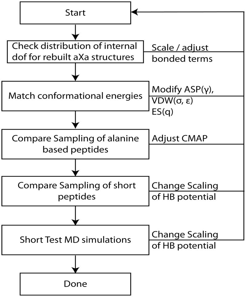
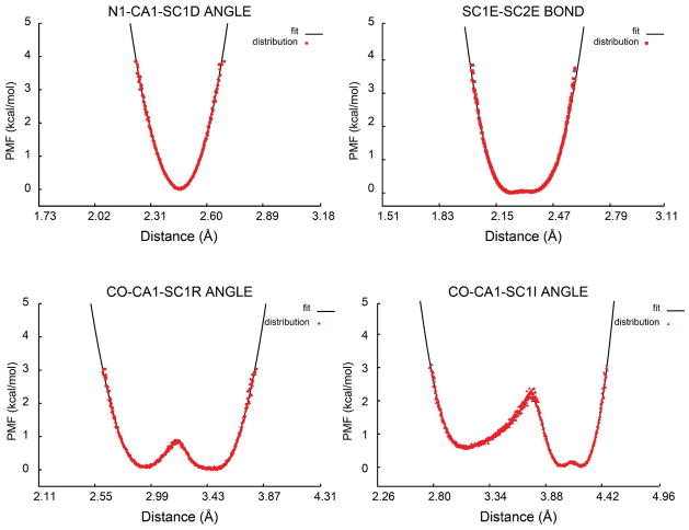
An overview of the optimization procedure is shown in the flowchart in Figure 2. The first step is the parameterization of the bonded terms. PMFs for bond, angle, and torsion terms were extracted from explicit solvent CHARMM dipeptide simulations and subsequently used to either fit a harmonic potential or generate a spline-interpolated potential for non-harmonic shapes (see Figure 3 and 4 for examples). The inverse-Boltzmann procedure is a common technique for generating coarse-grained potentials from atomistic data. However, different from previous approaches, we only use this method here for bonded interactions. The combination of various effective free energy terms always raises the issue of over-counting contributions and proper accounting of entropic effects. Here, we make the assumption that each of the bonded degrees of freedom are largely decoupled from each other and that the bonded terms are largely dominated by enthalpic rather than entropic effects. An additional assumption is that the effective bonded PMFs obtained for dipeptides in explicit solvent remain valid in longer peptides and condensed phase environments such as the interior of proteins. This assumption is most likely valid for bonds and angles, at least within the level of approximation expected for a coarse-grained model, but the treatment of torsion angle terms may be somewhat problematic in this respect. Therefore, the initial parameterization based on CHARMM simulation results was followed by further adjustments to match the results from PRIMO simulations for AXA tripeptides with results from CHARMM dipeptide simulations.
Figure 2.
Flowchart depicting the PRIMO force field parameterization scheme.
Figure 3.
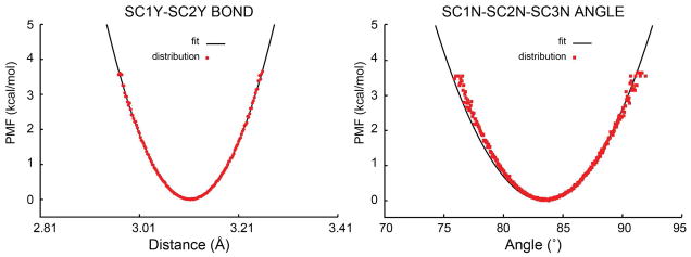
An example of the PRIMO harmonic potential (black) for bonds and angles fit into corresponding CHARMM explicit dipeptide simulations (red). Left: bonded term between SC1 and SC2 particles of tyrosine; right: angle term between SC1, SC2, and SC3 particles of asparagine.
Figure 4.
Distance spline potentials for bond and angle terms. The spline potential (black) is fitted to the sampling (red) from CHARMM dipeptide simulations. Top left: for N1, CA1, and SC1D angle of aspartic acid (N1-SC1D distance); top right: for SC1E-SC2E bond of glutamic acid; bottom left: CO, CA1, and SC1R angle of arginine (CO-SC1R distance); bottom right: CO, CA1, and SC1I angle of isoleucine (CO-SC1I distance).
Bonded terms involving virtual atoms were also parameterized based on a comparison of simulation results with PRIMO and CHARMM. As an example, Figure 5 shows the initial distribution of the cα-cβ-cγ angle in the AFA peptide using PRIMO (after reconstruction; in blue) in comparison with the atomistic results. The harmonic potential involving the virtual atoms was then adjusted to obtain the improved distribution (in green). The resulting improved potential does not match perfectly with the corresponding CHARMM result as a consequence of keeping a relatively weak harmonic potential involving virtual atoms to avoid distortions of the CG potential otherwise.
Figure 5.
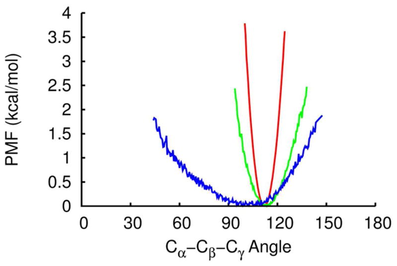
Sampling of the angle cα-cβ-cγ for phenylalanine with or without the potential CA1-cβ*-SC1. Red: sampling from all-atom simulations; green: with virtual site potential; blue: without virtual site potential.
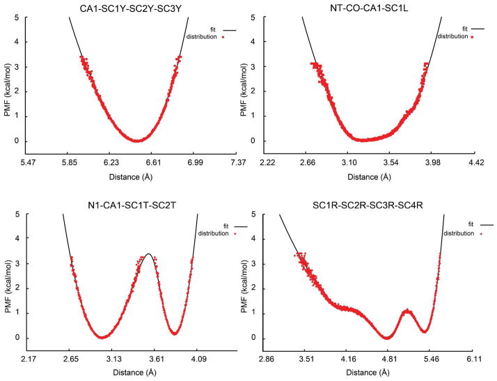
Similarly, except for a torsional potential corresponding to the peptide bond CA1-CO-N1-CA1, which is the same as the CHARMM cα-c-n-cα torsion, all other torsions were implemented as 1–4 distance based spline terms (see examples in Figure 6). The initial PMFs obtained from the atomistic MD were smoothened and in a few cases the barrier heights between two minima were reduced to obtain numerically well-behaved potentials that allow larger time steps to be used. A detailed discussion of the sampling of internal degrees of freedom in the reconstructed structures is provided in the result section as well as Supplementary Information.
Figure 6.
Different types of distance-based 1–4 spline potentials used in PRIMO (black) for torsional potentials fitted to corresponding CHARMM dipeptide simulations (red). Top left: rotation about SC1Y-SC2Y bond of tyrosine (CA1-SC3Y distance); top right: rotation about the CO-CA1 bond of leucine (N of next residue and SC1L distance); bottom left: rotation about the CA1-SC1T bond of threonine (N1-SC2T distance); bottom right: SC2R-SC3R bond of arginine (SC1R-SC4R distance).
The non-bonded parameters (qi, εij, σij, γi) in PRIMO were tuned by matching conformational energies for decoy sets with the corresponding CHARMM energies. The initial parameters for all εij values were set to −0.1 kcal/mol (−0.05 kcal/mol for ELJ1–4). However, for alanine, the parameters for the backbone N1 and CA1 were chosen based on CHARMM C19 and CO was set initially at −0.12 kcal/mol. The initial values for σij, were calculated from constituent atomistic beads based on a grid-based approach. The idea was to approximate the volume occupied by the constituent atoms with a spherical CG bead of radius σ, determined by counting points on a radial grid. It is worth mentioning that the van der Waals potentials parameters in classical all-atom force field are usually extracted from classical molecular dynamics simulations of simple compounds in order to produce their vapor- or liquid-phase thermodynamic properties.
The initial guess parameters in the Lennard–Jones term (σij, εij), including reduced values for 1–4 interactions, were then optimized to reproduce CHARMM all-atom energies for a series of peptide test sets. However, the initial optimized values of the energy depth εij of LJ potentials were found to be inadequate for protein-protein interactions. The energy depths were later scaled to match the binding energy profile for all seven protein-protein complexes66.
In Figure 7 the van der Waals interactions energies are shown as a function of separation distance between chains A and B of the protein-protein complex 1GUA. It is evident from the figure that the initial optimized PRIMO parameters could not reproduce the CHARMM profile due to weak LJ-depths (εij) compared to CHARMM. Hence, they were scaled by a factor of three. The resulting binding energy profile (total energy as well as van der Waals energy) agrees well with the corresponding CHARMM profile as can be seen from Figure 7. A detailed discussion of the binding profiles for all seven complexes was provided in our previous publication66.
Figure 7.
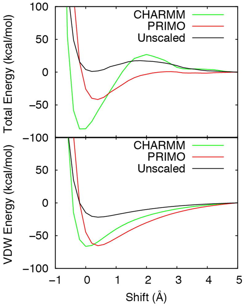
The binding energy profiles for the complex 1GUA obtained from CHARMM (green), PRIMO (red), and PRIMO with the unscaled LJ well depths (black).
Electrostatic interactions involve partial charges for each PRIMO site. Figure 1 depicts the charges (color-coded) in PRIMO. Initial charges were guessed based on the CHARMM19 or CHARMM22 force field and subsequently optimized. Total charges per amino acid were required to have integral charges of −1, 0, and +1 depending on the amino acid type. Furthermore, the goal was to preserve chemical specificity by placing most of the charge on polar groups but unlike MARTINI, charges were distributed over several CG particles to reduce artifacts.
Because of the coarse-grained nature of our model, the partial charges are generally reduced over all-atom models albeit formal charges are maintained for acidic and basic amino acids. Because of the reduced charges, all-atom electrostatic interactions are not accounted for completely so that the PRIMO charges cannot be optimized directly by simply fitting to all-atom electrostatic energies. The hydrogen bonding potential was introduced to compensate for insufficient electrostatics due to reduced charges. Partial charges and scaling factors (f3, f4, f5, and fn in Eq. 13) for the PMF-based hydrogen bonding potential were then optimized conjointly by fitting total PRIMO internal energies (including bonded and non-bonded terms) to total CHARMM all-atom energies for a series of test peptides. Later, the scaling factors for H-bonding potential were further tuned by carrying out MD simulations of villin and protein L until stable trajectories were obtained for these two proteins. The resulting optimized values for f3, f4, f5, and fn are 0.35, 0.50, 0.35, and 0.75, respectively. The resulting PMFs for the hydrogen bonding potential is shown in Figure 8.
Figure 8.
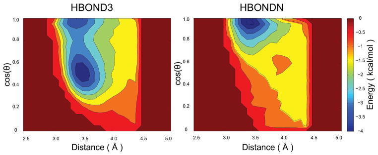
PMF for distance- and angle-based hydrogen bonding potential. Left: interaction between residues i and i + 3, right: interaction between residues i and i + n where n > 3.
The approach taken here differs somewhat from approaches taken in the development of other CG models. For example, in the case of SCORPION (solvated coarse-grained protein interaction) model67, the CG point charges were optimized for a given protein to generate a potential which best fits, in a least-square sense, the vacuum electrostatic potential created by the partial charges of the all-atom model, on a 3-dimensional grid outside the protein. Although a separate fitting of the electrostatic term is more rigorous, we did not think that the reduced resolution of our model would justify such an approach and was more likely to introduce artifacts because of over- or under-polarization.
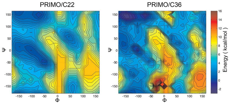
Following the initial adjustment of bonded and non-bonded terms, simulations of alanine-based peptides were generated with PRIMO to compare the sampling of backbone torsion angles ϕ and ψ with CHARMM. A map-based spline interpolated cross-correlation term (CMAP) was then introduced in PRIMO to match CHARMM secondary structure propensities. The spline potential is specified by energies determined on a 2D lattice with a 15° grid spacing. Initially, the CMAP potential was matched to the CHARMM22/CMAP force field (Fig. 9) but a second map was also generated to match the altered backbone torsion sampling with the new CHARMM C36 force field59,60. CMAP potentials were also generated for proline and glycine dipeptides (see Figure 10).
Figure 9.
CHARMM22/CMAP-based (left) and CHARMM36/CMAP-based (right) PRIMO-CMAP for nonglycine and nonproline residues. Colors indicate relative free energies according to color bar given on the right.
Figure 10.
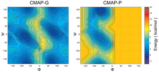
CMAP potential for glycine (left) and proline (right). Colors indicate relative free energies according to color bar given on the right.
Finally, the implicit solvent model was parameterized. The GBMV model is essentially parameter-free with respect to using it with different force fields – except for the atomic radii used to define the molecular surface. Standard Lennard-Jones radii were used for most atoms but the radii for acidic and charged residues were adjusted slightly to match the energetics of the atomistic model when implicit solvent is included. In the ASP part of the solvation term, all of the γi values were considered adjustable parameters. The main criterion for fitting the ASP coefficients was a comparison between combined GB and ASP energies in PRIMO to all-atom implicit solvent free energies.
PRIMO allows the use of blocked termini through N-terminal acetylation (ACE) and C-terminal N-methyl amide (CT3). The required parameters were not optimized separately, but rather taken from similar CG types. For example, in the case of ACE, SCT or SNT corresponds to CH3 with parameters that are similar to SC1A or CA1 (for the dihedral potential). Similarly, in the case of CT3, COY is used for CO and NT is used for N1 in PRIMO.
5. Simulation methods
MD simulations with PRIMO were carried out with blocked termini using the force field described above. A temperature of 300K was maintained with the Langevin thermostat using a friction coefficient of 10 ps−1. Equations of motion were integrated using the leapfrog Verlet integrator with a time step of 4 fs. Non-bonded interactions were cut off at 17 Å, with smooth switching to zero starting at 14 Å. The non-bonded interaction list was maintained up to 20 Å.
The equilibration protocol for all of the simulations generally consisted of initial minimization followed by stepwise heating to 300 K. During the heating phase, heavy atoms were kept fixed with a harmonic constraint, but production simulations were carried out completely unrestrained. PRIMO simulations were carried out using version c36a4 of the CHARMM molecular dynamics program package68. All analyses were performed using the MMTSB (Multi-scale Modeling Tools for Structural Biology) Tool Set69 in conjunction with CHARMM.
6. Results and Discussions
Results are first described for the training sets and then for a number of test sets where PRIMO was applied after the parameterization was completed.
6.1 Training Sets
Comparison of sampling of internal degrees of freedom in AXA and CHARMM dipeptide simulations
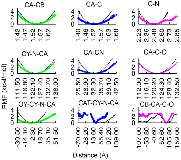
The bonded interactions in PRIMO were parameterized based on PMFs extracted from all-atom MD simulations. However, it is not obvious that this translates into accurately reproduced interaction profiles between all atomistic sites after reconstruction from PRIMO. To examine this point, PRIMO simulations of AXA peptides were compared with dipeptide simulations using CHARMM.
Typical results are shown in Figure 11 where PMF profiles of various internal degrees of freedom for residue 2 in AAA are compared between CHARMM and PRIMO. Data for other residues are provided in the Supporting Information. These distributions were generated after reconstructing the trajectory back to all-atom level of detail. Overall, there is good agreement but some deviations are apparent. In general, there is a trend of softer bonded interactions with PRIMO compared to the PMFs from CHARMM. This is likely a consequence of the smoother energy landscape in the CG model due to fewer degrees of freedom. For some of the torsion angles the deviations appear to be more significant although the overall shape is still maintained and only the relative populations between different states differ, e.g. for the CB-CA-C-O torsion. Because this analysis depends on reconstructed atoms, it is likely, though, that not just the inherent energetics and dynamics of the PRIMO model plays a role but also the accuracy of the reconstruction procedure.
Figure 11.
Distributions of internal degrees of freedom for AAA. Upper panel: bonds; middle panel: angles; lower panel: dihedral angles.
PRIMO versus CHARMM Free Energies for Decoy Sets
Non-bonded parameters in PRIMO were optimized by matching the free energies from PRIMO to CHARMM implicit solvent free energies for a series of different decoy sets. The results presented here reflect the final, optimized parameter set. In many cases, better results could have been obtained for any individual data set but at the expense of other data sets. Therefore, deviations from the CHARMM reference indicate the compromises that have been made in the development of PRIMO.
Table 2 lists the solvation free energies obtained from PRIMO and CHARMM with GBMV for dipeptides with different side chains. The solvation free energy obtained from PRIMO generally agrees well with the corresponding CHARMM result indicating that the solvation of different amino acids is well balanced. However, PRIMO significantly overestimates the unsigned solvation free energy for the glutamic acid (Glu) and histidine dipeptides.
Table 2.
Comparison of solvation free energies for dipeptides obtained from PRIMO and CHARMM with GBMV simulations. The correlation coefficient varies between 0.3 and 0.6.
| AA | ΔGCHARMM (kcal/mol) | ΔGPRIMO (kcal/mol) | ΔΔG(a) (kcal/mol) |
|---|---|---|---|
| Ala | 17.2 | 16.5 | −0.7 |
| Arg | −54.4 | −57.4 | −3.0 |
| Asn | 6.9 | 10.3 | 3.4 |
| Asp | −55.3 | −55.3 | 0.0 |
| Cys | 15.4 | 17.2 | 1.8 |
| Gln | 7.2 | 8.7 | 1.5 |
| Glu | −56.9 | −69.2 | −12.3 |
| Gly | 14.8 | 17.1 | 2.3 |
| Hsd | 5.3 | 11.0 | 5.7 |
| Hse | 6.0 | 11.0 | 5.0 |
| Ile | 18.6 | 18.0 | −0.6 |
| Leu | 17.8 | 17.2 | −0.6 |
| Lys | −63.9 | −64.0 | −0.1 |
| Met | 17.4 | 16.7 | −0.7 |
| Phe | 16.6 | 17.4 | 0.8 |
| Pro | 18.6 | 19.4 | 0.8 |
| Ser | 11.7 | 11.9 | 0.2 |
| Thr | 14.0 | 11.9 | −2.1 |
| Trp | 14.0 | 13.4 | −0.6 |
| Tyr | 11.5 | 11.5 | 0.0 |
| Val | 17.5 | 16.9 | −0.6 |
ΔΔG = ΔGPRIMO − ΔGCHARMM
Figure S6 depicts PRIMO versus CHARMM free energies for (AAXAA)4 decoys along with respective correlation coefficients. The data shows that the free energies from PRIMO are highly correlated to CHARMM with a correlation coefficient varying between 0.63 and 0.97. The lowest correlation is obtained for (AAPAA)4 while the highest correlation corresponds to (AAAAA)4 decoy sets. The low correlation for (AAPAA)4 is a result of a narrower distribution of conformations because the peptide is more restricted with proline. The slope ranges between 0.73 and 1.36 indicating that the relative energy differences between different conformations largely have the correct magnitudes compared to CHARMM.
In Figure 12 we have compared PRIMO energies with CHARMM for the villin and protein L decoy sets. Although the absolute energies differ between PRIMO and CHARMM, the energies are again highly correlated with a correlation coefficient of ~0.90. Furthermore, relative energies are again well reproduced. A slope of 1.09 is obtained for villin decoys while a slope of 0.92 is estimated for the protein L decoy sets.
Figure 12.
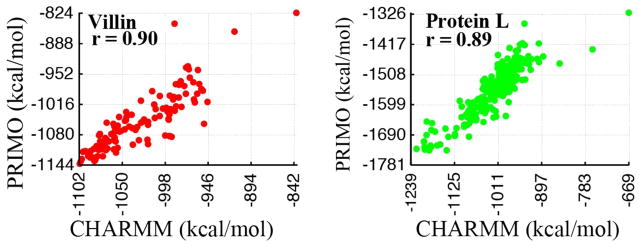
PRIMO versus CHARMM total energies for villin (left) and protein L (right) decoys with corresponding linear correlation coefficients r.
Next, we compared the binding free energies for all protein-protein complexes obtained from PRIMO and CHARMM (see Table 3). It is evident from the table that an accurate reproduction of protein-protein interaction energies may present the largest challenge for PRIMO. PRIMO underestimates the binding free energy for all complexes but 1HV2 and the deviations are on the order of tens of kcal/mol in some cases. Nevertheless, binding free energies profiles with PRIMO are overall highly correlated to CHARMM data (see Figure 7) and the correlation coefficient varies between 0.5 and 1.0. While the lowest (0.5) correlation coefficient is observed for the 2D1F decoy sets, a perfect correlation (1.0) is obtained for 1HV2. A plausible reason for obtaining right orders of magnitude for 2D1F and 1HV2, but not 2CIA and 2V8S could be that PRIMO was unable to recognize the correct bound structure for 2CIA and 2V8S while it could correctly differentiate between unbound and bound conformations in cases of 2D1F and 1HV2. We intend to further examine these test cases in future studies to improve the accuracy of PRIMO in reproducing the energetics of protein-protein interactions.
Table 3.
Binding free energies for protein-protein complexes obtained with PRIMO and CHARMM with GBMV representation.
| Protein | Correlation | ΔGCHARMM (kcal/mol) | ΔGPRIMO (kcal/mol) | ΔΔG(a) (kcal/mol) |
|---|---|---|---|---|
| 1GUA | 0.6 | 71.9 | 4.7 | −67.2 |
| 1HV2 | 1.0 | 4.4 | 9.2 | 4.8 |
| 2C5I | 0.8 | 9.0 | 2.4 | −6.6 |
| 2CIA | 0.6 | 21.8 | 0.1 | −21.7 |
| 2D1F | 0.8 | 6.1 | 6.0 | −0.1 |
| 2OEI | 0.8 | 27.5 | 0.5 | −27.0 |
| 2V8S | 0.8 | 7.9 | 0.1 | −7.8 |
| 3BS5 | 0.5 | 39.0 | 1.8 | −37.2 |
ΔΔG = ΔGPRIMO − ΔGCHARMM
Although far from perfect, the energetic agreement between PRIMO and CHARMM is overall remarkable considering the different levels of resolution with a reduction in interaction sites by a factor of about 3. We are not aware of a similar level of energetic correspondence between atomistic and coarse-grained models for other CG models that have been proposed previously.
ϕ/ψ Sampling in AXA Simulations
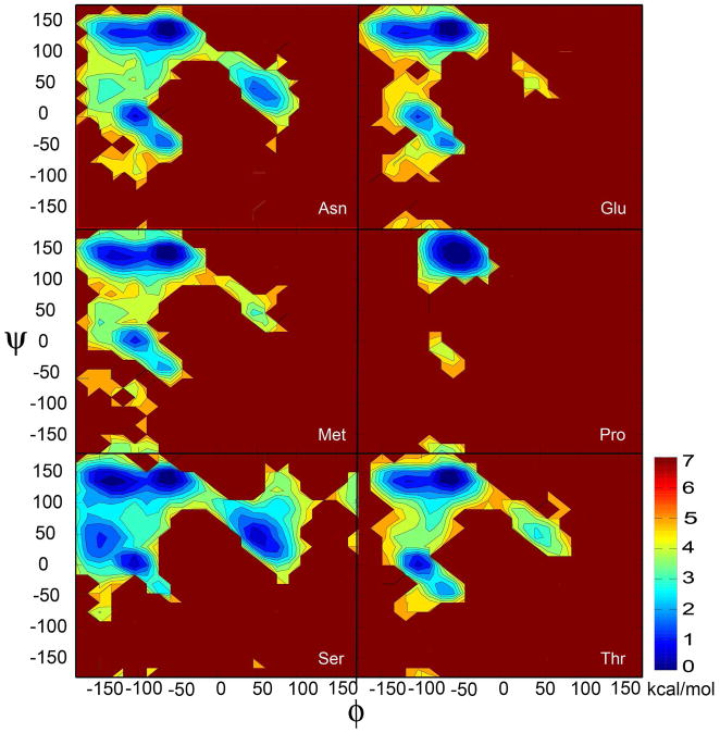
The conformational preference for different ϕ (C-N-Cα-C)/ψ (N-Cα-C-N) backbone torsion angles is a key determinant for forming different secondary structure elements. For the all-atom representations, the Ramachandran plot (RP) is used to validate the backbone conformation of a protein model. To validate a protein model, the protein RP must not display anomalies, such as points in the forbidden regions. Furthermore, the preference for different secondary structure elements is highly sensitive to the relative sampling of the corresponding regions in the RP. PRIMO is designed to provide a correct description of conformational distribution of the backbone (ϕ/ψ) for all amino acids due to the CMAP correction term. To validate this assertion, the distribution of ϕ/ψ torsion angles from blocked AXA simulations was studied as a function of the amino acid type. Blocked AXA tripeptides were chosen because they can serve as prototypes of non-glycine/non-proline protein backbones with full sampling of the ϕ/ψ conformational space without the additional complexity of side chain degrees of freedom. Results for selected amino acids are shown in Figure 13 while data for other amino acids are shown in the Supporting Information (Figure S7). Feig65 obtained a similar distribution in the case of dipeptide simulations with the CHARMM22/CMAP force field.
Figure 13.
Potentials of mean force for the sampling of ϕ/ψ backbone torsion angles in selected amino acid residues from AXA simulations. A color bar indicating energy levels is provided on the right.
In general, as in the previous study65, it appears that in the β basin, most of the amino acids follow a similar energy landscape with two minima near C5 and PPII that are connected by a very shallow barrier. The fully extended conformations near C5 are slightly less favorable compared to PPII conformations. Furthermore, as in the dipeptide simulations65, sampling of the C7eq conformation near (ϕ = −75, ψ = 75) in the α/β transition region appears to be too unfavorable, which is especially apparent in aspartic acid, leucine, and proline. In asparagine, serine, histidine, cytosine, glutamine, and lysine and to a lesser extent in tryptophan, there is a third minimum in the simulations near (ϕ = −150, ψ = 40). In proline, although the major minimum at PPII is sampled, the C7eq or αR conformations are not favorable enough. This finding matches qualitatively the results with CHAMM22/CMAP for proline dipeptide in explicit solvent65.
For asparagine, the sampling of αL conformations is relatively favorable while it is relatively unfavorable for threonine, glutamic acid, and methionine, which is again in good agreement with the dipeptide simulations or PDB distributions65. Aspartic acid predominantly samples αR (ϕ = −60, ψ = −50) while all other amino acids sample predominantly a minimum at (ϕ = −100, ψ = 0). A similar trend was observed previously in the dipeptide simulations65. Finally, we do not see any sampling in C7ax (ϕ = 50, ψ = −130) region, which is in contrast to what was observed by Feig58 in the dipeptide simulations.
The results in Figure 13 show that the ϕ/ψ preferences vary only to a small degree among different amino acids, suggesting that amino acid dependent variations in ϕ/ψ preferences do in fact stem predominantly from interactions due to polypeptide and protein environments. However, closer inspections reveal some differences among different amino acids. Next, we characterize these subtle variations in ϕ/ψ preferences among different residues quantitatively (see Table 4). The relative sampling of the α basin varies between 3 and 16 % and the ratios of αR to α′ are mostly below 1, which indicates that the sampling of αR is relatively disfavored in the tripeptides, which is in good agreement with the previous observation made by Feig65 in the dipeptide simulations. However, aspartic acid predominantly samples the αR basin over α′. Asparagine, aspartic acid, serine, and threonine in the AXA simulations sample nearly 16% while remaining amino acids spend 3 to 10% of the time in the α basin. The relative sampling of the β basin in the AXA simulations is measured to be at or below 95% for most of the amino acids but serine, asparagine, and aspartic acid. Serine spends the lowest time (65%) in the β basin while the highest sampling (95%) is observed for leucine. The preference for sampling in the α-basin versus β-basin matches to a large extent with the dipeptide simulations65.
Table 4.
Relative sampling (in %) of different regions in the Ramachandran plot for each amino acid in AXA.
| Amino acids | α(αR/α′) | β | αL |
|---|---|---|---|
| Ala | 6 (0.51) | 90 | 3.2 |
| Arg | 7 (0.20) | 92 | 0.5 |
| Asn | 16 (0.29) | 76 | 7.0 |
| Asp | 12 (17.94) | 70 | 18.1 |
| Cys | 8 (0.24) | 91 | 0.4 |
| Gln | 10 (0.13) | 88 | 1.0 |
| Glu | 9 (0.57) | 91 | 0.1 |
| His | 10 (0.20) | 88 | 1.4 |
| Ile | 10 (0.17) | 88 | 1.3 |
| Leu | 3 (0.74) | 95 | 2.2 |
| Lys | 8 (0.17) | 91 | 1.0 |
| Met | 8 (0.18) | 92 | 0.3 |
| Phe | 9 (0.21) | 90 | 0.6 |
| Ser | 14 (0.03) | 65 | 17.4 |
| Thr | 16 (0.12) | 83 | 0.9 |
| Trp | 6 (0.36) | 94 | 0.2 |
| Tyr | 8 (0.18) | 92 | 0.4 |
| Val | 5 (0.69) | 91 | 4.2 |
Samplings on the right-hand side of the RP are important for the formation of turns. The αL conformations are sampled at widely varying levels in the PRIMO tripeptide simulations. Aspartic acid and serine in the AXA simulations spend nearly 18% of the time in the αL basin, while alanine, asparagine, and valine spend 3 to 7% of the time in the αL basin. For glutamine, histidine, isoleucine, leucine, and lysine, the relative sampling in the αL basin varies between 1 and 2 % while remaining amino acids essentially never sample αL. It is worth noting that the relative sampling of αL conformations in PRIMO is in good qualitative agreement with the PDB distributions65.
Overall, PRIMO samples the major minima in the RP and captures the subtle but significant residue type-dependent variations in ϕ/ψ preferences at the tripeptide level and qualitatively agree well with the previous study65.
Conformational Sampling of short peptides
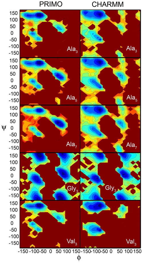
As the CMAP potential in PRIMO is optimized based on sampling of alanine-based short peptides, we describe here the conformational sampling of these short peptides and compare with the corresponding CHARMM results58. The peptides Ala3, Val3, and Gly3 were simulated at 300 K for 500 ns while replica exchange molecular dynamics (REMD) simulations were conducted for Ala5 and Ala7. For both peptides, 12 replicas were used with a temperature range 270–500 K. For both cases, exchanges between two consecutive replicas were attempted in every 10 ps, leading to an acceptance ratio of ~80%. Each replica was simulated for 300 ns.
The ϕ/ψ sampling for Ala3, Ala5, Ala7, Val3, and Gly3 is shown in Figure 14 and compared to the distribution from explicit solvent, atomistic CHARMM C36 simulations. The agreement between the results from PRIMO and CHARMM is remarkably good, especially in the major conformational basins. Similar to CHARMM, the dominant minimum in alanine- and valine-based peptides lies at PPII (ϕ = −60, ψ = 140) but additional minima at C5 and αR are only slightly higher in energy. In both force fields, a very shallow energy barrier connects the two minima near C5 and PPII. Overall, conformations near αR basins are slightly too favorable in PRIMO over α′(ϕ = −160, ψ = 0) conformations. This observation is in contrast to what has been observed for most of the PRIMO tripeptide, indicating that the sampling of αR conformations is relatively disfavored in tripeptides. However, this agrees with the CHARMM36/CMAP simulations of the same polypeptides. Therefore, the polypeptide context and, in particular, the ability to form i, i + 4 backbone hydrogen bonding is essential in stabilizing α-helical secondary structure element. The sampling of the C7eq conformation near (ϕ = −75, ψ = 75) in the α/β transition region, however, appears to be less favorable in the case of PRIMO compared to CHARMM, which is especially apparent in Ala7.
Figure 14.
Sampling of ϕ/ψ torsion angles in the central residues of Ala3, Ala5, Ala7, Val3, and Gly3 with the PRIMO force field (left column) and the CHARMM36 force field (right column). Data corresponding to CHARMM simulations were obtained from Ref. 52. Colors indicate relative free energies according to color bar given on the right of Figure 16.
Conformations on the right-hand side of the RP are important for the formation of turns. An additional minimum at αL is about 2–3 kcal/mol higher than the PPII conformation, which is again in good agreement with the CHARMM results. In general, an overall increased preference for αL conformations compared to the CHARMM simulations is observed in PRIMO. Interestingly, an additional minimum at C7ax is absent in alanine-based polypeptide that is present in the new CHARMMC36/CMAP. Gly3 exhibits symmetric sampling with similar minima at αR/αL and PPII/C7ax and agrees remarkably well with the corresponding CHARMM sampling.
There are subtle differences among Ala3, Ala5, and Ala7 but the overall trend in variations among different regions of the RP is very similar. The ability of PRIMO to sample different major minima in the RP for alanine-based polypeptides agrees qualitatively very well with the CHARMM simulations. Subtle differences between PRIMO and CHARMM may be expected since the PRIMO simulations are not just based on a reduced representation of the peptides but also used implicit solvent whereas the corresponding CHARMM simulations were conducted in explicit water with an all-atom description of the peptides.
6.2 Test Results
The optimized force field was further applied to a number of test cases to assess the ability of PRIMO to reproduce structural and dynamic properties in comparison with experimental data and other simulations using all-atom force fields.
6.2.1 PRIMO-MD Simulations
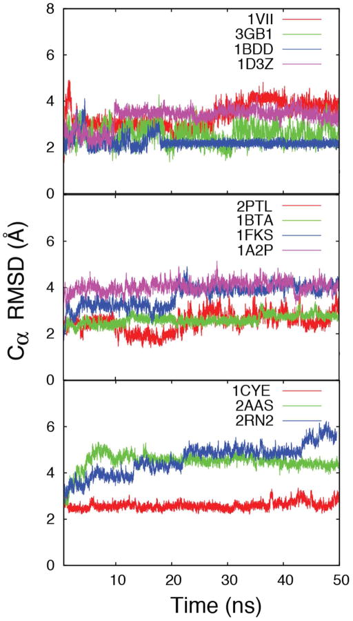
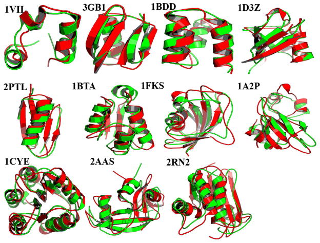
A major goal of PRIMO is to be able to run stable MD simulations of arbitrary protein systems. PRIMO was tested on a set of 11 proteins with 36–155 amino acids (see Table 5). All protein simulations were started from the experimental structures and simulated with blocked termini for 50 ns. Figure 15 shows the Cα RMSD of all proteins as a function of simulation time with respect to their experimental structures, and it is evident from the figure that the most of the proteins reach their stable conformations within the first 10 ns and the Cα RMSDs are kept within 3.5 Å for most proteins. Since it may appear that the MD sampling for the two proteins 1VII and 2PTL has not reached convergence within 50 ns these simulations were extended to 100 ns (see Figure S8). On average, the RMSDs did not increase significantly during 50–100 ns. Average Cα RMSD values during the simulation as well as Cα RMSD of the average structure over the entire trajectory are reported in Table 5. These values are compared with the CHARMM all-atom simulations of the same set of proteins in explicit water. As is well known, the RMSD of the average structure is lower than the average instantaneous RMSD values as it corresponds more closely to the experimental scenario65. Therefore, we will focus the discussion on those values. For PRIMO, the RMSD varies between 1.80 and 4.03 Å compared to CHARMM, which varies between 0.79 and 2.74 Å65. The explicit solvent simulations used for comparison here result from using the CHARMM22/CMAP force field65 but results from Best et al.58 indicate that similar results are expected for the newer force field CHARMM/C36. In the PRIMO MD simulations, two proteins have deviations below 2 Å and four additional proteins are between 2 and 3 Å. Out of the remaining five other proteins, the RMSD is found to be between 3 and 4 Å for four systems and only one system is just above 4 Å. The larger RMSD in 2AAS can be attributed to the presence of flexible loop regions (residues 20–25 and 58–61) that may be sampled more extensively in the CG model relative to CHARMM since the kinetic time scales between the all-atom and CG models are expected to differ. Both loops are located at the solvent-exposed surface of the protein, so they are less stable compared to the secondary structure and the hydrophobic core of the protein during the simulation. In general, the RMSDs with PRIMO-MD are larger than those found with all-atom MD simulations, but their values are comparable, and the average Cα RMSD of 1FKS is even lower. Figure 16 shows a superposition of the average structures generated from our simulations with the corresponding experimental structure. As can be seen, the structural variations are generally small and typically involve minor rearrangements of loops and helices, most notably at the flexible N- or C-termini. Overall, these results demonstrate that, in general, PRIMO can maintain experimental structures of proteins well.
Table 5.
Root mean square deviations from experimental structures in PRIMO-MD simulations compared with all-atom simulations. Standard deviations are provided in parentheses.
| PDB | Res | avg. Cα RMSD (PRIMO) (Å) | Cα RMSD of avg. structure (PRIMO) (Å) | avg. Cα RMSD (CHARMM) (Å) | Cα RMSD of avg. structure (CHARMM) (Å) | RgPRIMO (Å) | RgCHARMM | Rgexp (Å) |
|---|---|---|---|---|---|---|---|---|
| 1VII | 36 | 3.3 (0.6) | 2.9 | 2.4 (0.4) | 2.3 | 9.4 (0.2) | 9.4 (0.2) | 9.4 |
| 3GB1 | 56 | 2.6 (0.5) | 2.3 | 1.1 (0.2) | 0.8 | 10.9 (0.1) | 10.4 (0.1) | 10.9 |
| 1BDD | 60 | 2.2 (0.3) | 1.8 | 2.0 (0.2) | 1.6 | 9.9 (0.1) | 9.4 (0.1) | 9.7 |
| 1D3Z | 76 | 3.3 (0.5) | 3.1 | 1.4 (0.2) | 1.3 | 11.9 (0.2) | 11.5 (0.1) | 12.0 |
| 2PTL | 78 | 2.5 (0.5) | 1.9 | 1.6 (0.3) | 1.3 | 11.6 (0.1) | 11.3 (0.1) | 11.5 |
| 1BTA | 89 | 2.6 (0.3) | 2.2 | 1.3 (0.2) | 1.2 | 12.1 (0.1) | 12.0 (0.1) | 11.8 |
| 1FKS | 107 | 3.5 (0.6) | 3.0 | 3.6 (0.7) | 2.7 | 13.1 (0.4) | 13.3 (0.2) | 13.7 |
| 1A2P | 110 | 3.9 (0.3) | 3.8 | 1.5 (0.3) | 1.2 | 14.0 (0.2) | 13.6 (0.1) | 13.6 |
| 2AAS | 124 | 4.4 (0.6) | 4.0 | 2.5 (0.4) | 2.0 | 14.9 (0.2) | 14.5 (0.2) | 14.2 |
| 1CYE | 129 | 2.6 (0.3) | 2.4 | 1.4 (0.2) | 1.2 | 13.4 (0.1) | 13.4 (0.1) | 13.3 |
| 2RN2 | 155 | 4.4 (0.6) | 3.8 | 2.0 (0.2) | 1.6 | 15.9 (0.2) | 15.3 (0.1) | 15.6 |
Figure 15.
Time evolution of Cα RMSD during PRIMO MD simulations selected proteins from their respective crystal structure.
Figure 16.
Superposition of average structure (green) for selected proteins obtained from PRIMO-MD simulations onto the corresponding crystal structures (red).
We have further calculated the radii of gyration for all proteins obtained from our simulations and compared it with the experimental values and CHARMM all-atom simulations. Good agreement is evident from the results shown in Table 5. It should be noted that the deviations from experiment are comparable to the fluctuations in the radii of gyration during the simulation. This suggests that PRIMO maintains good packing of the protein chains at the coarse-grained level.
Finally, we also estimated the solvent accessible surface area (SASA) for all proteins, which is more sensitive to smaller changes of surface-exposed regions. Table S3 (Supplementary Information) compares the PRIMO results with results from CHARMM as well as experimental results. The agreement between PRIMO and CHARMM (and the experimental values) is good for most proteins but in some cases, there are more significant deviations. The average SASA obtained from PRIMO simulations is always larger than the CHARMM or the experimental value except for 1VII. The worst case is 2RN2 where the SASA increases by 1000 Å2. This suggests that although the overall packing appears to be maintained, since the radii of gyration match well, structural elements near the surface may exhibit a slight tendency to more exposure in PRIMO.
PRIMO versus other CG Force Fields
It is instructive to compare the performance of our PRIMO force field with other recent CG force fields. Using a set of 956 proteins and a two-bead model, Majek and Elber19 found that 58% of the proteins stayed within 5 Å Cα RMSD from their native structures during 20 ns at 300 K. Tested on eight proteins with 17–98 amino acids, the three-bead model developed by Basdevant et al.15 yielded Cα RMSDs varying between 3 and 8 Å from the experimental structures during 200 ns at 300 K. Pasi and co-workers48 have observed that the equilibrium trajectories remain in the neighborhood of the native structure, with average RMSD values between 3.9 and 4.6 Å. Gu et al.70 have recently studied eight out of eleven proteins listed in Table 5 with the MARTINI model for 10 ns. They have observed that the average Cα RMSD for eight proteins varies between 3.39 and 5.03 Å. With PRIMO, we observe a range between 1.80 and 4.03 Å for the same set of proteins. It should be noted here that the simulation times used in MARTINI were relatively short compared to PRIMO (10 ns versus 50 ns). Furthermore, information about the secondary structure had to be used as part of the MARTINI potential, while no such bias was necessary with the PRIMO CG model.
Recently Chebaro and co-workers36 have shown that OPEP4-MD simulations at 300 K preserve the experimental rigid conformations of 17 proteins with 37–152 residues with RMSDs varying between 2.1 Å and 3.6 Å during 30 ns. Because the performance of OPEP4 is similar to what we report here, we also tested PRIMO in MD simulations of the 17 proteins from the OPEP test set. The results are shown in Table S4 (Supplementary Information). As in the OPEP paper, we only report RMSD values for rigid core Cα atoms. Overall, the performance of PRIMO is comparable to OPEP4 in simulating folded proteins in their native environment. In our simulations, they vary between 2.8 to 3.8 Å for 14 proteins and 4.2 to 6.1 Å for three other proteins. The protein 2KTE shows the largest RMSD of 6.1 Å. The apparently large RMSD with the experimental structure (6.1 Å) is mainly due to small changes in the relative orientation of some of the α-helices. This comparison suggests that PRIMO may perform somewhat worse than OPEP4 but it is possible that the OPEP force field tends to over stabilize native states since it was optimized primarily based on its ability to discriminate the native structure from non-native structures. Another plausible reason could be an adequate balance between short-range and long interactions due to a new formalism for the van der Waals interactions and the inclusion of i, i + 3 interactions in helical proteins. PRIMO, on the other hand, was parameterized primarily based on small peptides and aims to balance folded, native and unfolded, non-native states.
Efficiency of the PRIMO Force Field
One of the main goals of coarse-graining is to improve the computational efficiency. In order to compare the computational efficiency, the above-mentioned eleven proteins were simulated for 1 ns with PRIMO, CHARMM/GBMV, and CHARMM/TIP3P, respectively. In the all-atom simulations, the CHARMM36 force field was used. All the simulations were performed in serial on an Intel E5-2680 processor (2.7 GHz). A 2 fs time-step was used for all-atom MD simulations while a time-step of 4 fs was used in the case of PRIMO. The simulation time is listed in Table S5 (Supporting Information). It is evident from the table that the simulation time is proportional to the system size for each simulation methodology. Compared to AA-MD simulations with GBMV representation, PRIMO can achieve about 8 to 12 speedup while about 10 to 20 speedup could be achieved with PRIMO compared to all-atom simulations with TIP3P water molecules. On the other hand, MARTINI can achieve about 75~100 speedup compared to AA-MD simulations for the same set of proteins70. A main bottleneck in PRIMO is the use of the GBMV methodology for treating solvent effects. Replacing the GBMV model with other, computationally more efficient GB implementations may greatly enhance the overall computational efficiency of PRIMO.
6.2.2 PRIMO-REMD
In the previous section, we have shown that the PRIMO force field is capable of maintaining the native structures of proteins in MD simulations. Here, we evaluate the applicability of the force field in folding simulations of peptides, and in particular to examine whether PRIMO is able to reproduce the correct balance between α-helical and β-sheet favoring peptides. Folding simulations of five small peptides were carried out using REMD simulations. A summary of all REMD simulations is provided in Table 6. As listed in Table 6, the peptides considered here include (1) α-helical peptides such as (AAQAA)3, AK17, and RNase C–peptide (CPEP); (2) β-hairpin peptides such as GB1, the N-terminal hairpin in the protein GB1 domain, GB1m2, a mutant variant of the same peptide, and trpzip2. For each system, the sequence, the number of replicas, the simulation time per replica, the temperature range, and the time interval used for analysis are reported in the table. All the simulations were started from an extended linear conformation and all peptides were studied in their blocked forms. The REMD simulations spanned a temperature range of 270 to 500 K with exponentially spaced 12 replicas for all. In all cases, exchanges between two consecutive replicas were attempted every 10 ps, leading to an acceptance ratio of 40–50%. The first 50 ns of each simulation of β-hairpin forming peptides were discarded while the initial 30 ns were discarded for the faster-folding helix-forming peptides.
Table 6.
Overview of PRIMO-REMD peptide folding simulations.
| system | sequence | time (ns) | # replicas | T range (K) | time for analysis (ns) |
|---|---|---|---|---|---|
| AQA | (AAQAA)3 | 100 | 12 | 270–500 | 30–100 |
| AK17 | (AAKAA)3GY | 100 | 12 | 270–500 | 30–100 |
| GB1 | GEWTYDDATKTFTVTE | 200 | 12 | 270–500 | 50–200 |
| GB1m2 | GEWTYNPATGKFTVTE | 200 | 12 | 270–500 | 50–200 |
| trpzip2 | SWTWENGKWTWK | 150 | 12 | 270–500 | 50–150 |
| C–peptide | KETAAAKFERQHM | 100 | 12 | 270–500 | 30–100 |
Folding of Helical Peptides
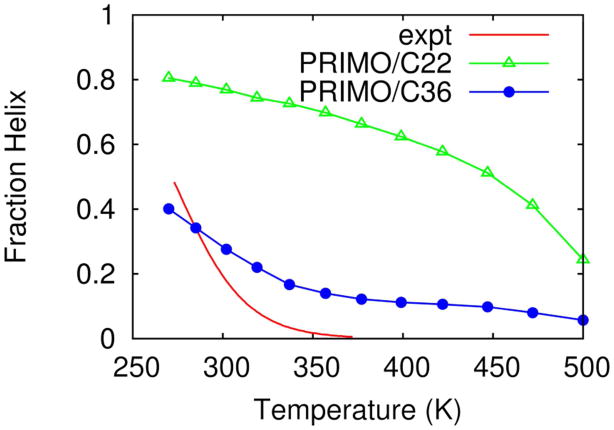
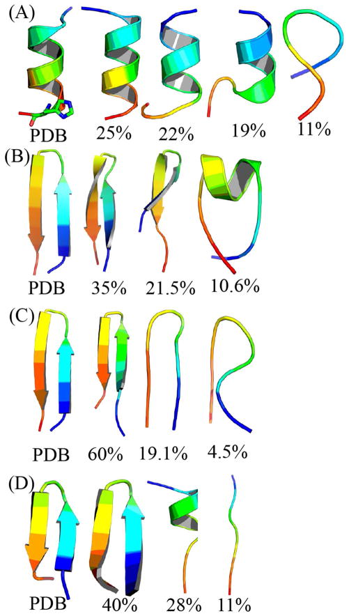
The first peptide that was studied was (AAQAA)3. This peptide was also used to tune the CHARMM/C36 force field58,59. Here we have studied this peptide using our coarse-grained force field in conjunction with the CMAP based on CHARMM/C22 and CHARMM/C36. The overall fraction of helicity, as measured by DSSP, at 270 and 300 K was found to be ~39% and ~24%, respectively. This agrees reasonably well with the experimental estimates of ~47% and ~19%71, respectively. It also agrees well with a 21% fraction of helicity at 300 K obtained with the CHARMM36/CMAP force field59. Furthermore, 95% helicity were found with the CHARMM22/CMAP force field58 whereas PRIMO using a CMAP based on the CHARMM22/CMAP force field resulted in 81% helicity indicating that PRIMO closely mimics the general characteristics of the underlying force field. In contrast, the OPEP4 coarse-grained force field underestimates the overall helix content and yields a helicity of only ~28% at 269 K72.
A noteworthy feature is revealed from Figure 17 where we have shown the overall helical content of (AAQAA)3 as a function of temperature. It is evident from the figure that the temperature dependence of the transition–which was not part of the force field optimization–is also in satisfactory agreement with experiment. The transition is cooperative and occurs over a small temperature range, as in experiment. A similar trend was also observed for CHARMM36/CMAP simulations. However, this trend was absent in CHARMM22/CMAP, PRIMO/C22 and AMBER simulations58. This further demonstrates that PRIMO responds to changes in the CMAP potential in a similar way as the atomistic force field.
Figure 17.
Helical content of the (AAQAA)3 peptide as a function of temperature calculated from PRIMO-REMD simulations with CMAPs based on CHARMM22 (green, triangles) and CHARMM36 force fields (blue, circles) and from experiment (red, line).
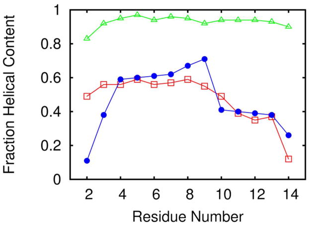
The helicity as a function of residue is shown in Figure 18. We compare the calculated residue helicity at 270 K with that derived from NMR chemical shift measurements at 274 K. It is evident from the figure that the average per-residue helical content of the peptide corresponding to the PRIMO/C22 simulations is much higher than that of experiment. On the other hand, residue helicity values obtained from PRIMO/C36 are highly correlated to the experimental data. In particular, we find that the helical contents in the middle of the helices are slightly higher than the helical contents closer to the termini as seen in experiment.
Figure 18.
Simulated vs experimental helicities as a function of residue for (AAQAA)3 with PRIMO/C22 (green, triangles), PRIMO/C36 (blue, circles), and from experiment (red, squares) at 270 K71.
Next, we were interested to see whether the optimized parameters can be transferred to other helical peptides. We therefore also carried out REMD simulations of a helical peptide [(AAKAA)3GY], known as the AK17 peptide, which has been studied experimentally73. The total helical content of the AK17 peptide at 300 K was estimated to be ~35.2% with PRIMO, averaged over the last 80 ns of 100 ns REMD simulations. This observation is consistent with ~30–35% of the helical content of this peptide by CD measurements73. The result also compares favorably with simulation results by Han et al.53 who reported the helical content to be ~41% for this peptide when they performed REMD simulations with their coarse-grained force field PACE.
Finally, we have studied the peptide CPEP corresponding to the first 13 N-terminal residues of Ribonuclease A (RNase A), which has a remarkably high α-helical propensity for a system of such a small size. According to CD measurements74, this peptide contains 50–60% helix at 276 K and pH 5.25. Based on NMR experiments, Osterhout et al.75 proposed that the conformational ensemble of RNase A C-peptide includes three principal conformations: a set of extended conformations, a set of largely helical conformations, and a set of conformations that contain a salt bridge between the side chains of Glu2 and Arg10.
In our PRIMO-REMD simulations, the helicity was found to be ~60% at 270 K while it is estimated as ~54% and ~49% at temperatures of 283 and 298 K, respectively. This observation agrees well with the experimental result74. The distribution of Cα RMSD from the experimental structure (pdb: 1RNU) shows that the peak of the most frequently visited conformations of the C-peptide is found to deviate by 2.5 Å at 270 K (Figure 19). Figure 19 furthermore suggests that our REMD simulations largely sample distinct conformations with Cα RMSDs of 2.5, 4 and 5.5 Å. The conformations generated at 270 K were clustered with a Cα RMSD cutoff of 4 Å using the K-means algorithm. In total, 12 clusters were identified, and the top four clusters are shown in Figure 20 along with the experimental structure. The populations of the four largest clusters are ~25%, ~22%, ~19%, and ~11% and they account for ~77% of the total populations. The largest cluster corresponds to a largely helical conformation while the fourth largest cluster corresponds to an extended conformation. A similar trend was also observed in experiments75. In the other two clusters, the peptides are also helical but the length of the helices differs from the structure with the largest cluster population. The melting temperature identified by a peak in the specific heat capacity profile, is estimated at 447 K, 422 K, and 400 K for (AAQAA)3, AK17, and CPEP, respectively.
Figure 19.
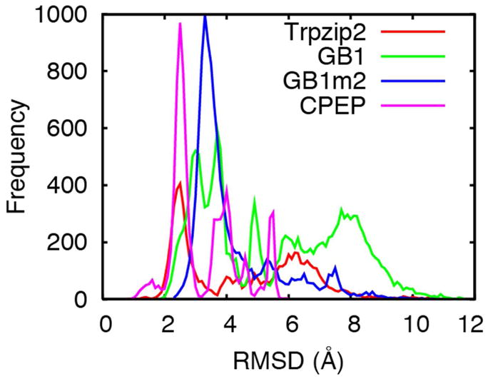
Distribution of Cα RMSD values for C-Peptide or CPEP (magenta), GB1 (green), GB1m2 (blue), and trpzip2 (red) in PRIMO REMD simulations.
Figure 20.
Representative structures of the most populated clusters of the C-peptide (A), GB1 (B), GB1m2 (C), and trpzip2 (D) peptides. Experimental structures (‘PDB’) are shown for comparison. The Cα RMSDs of the representative structures corresponding to the largest clusters were estimated to be 2.5, 3, 3.3, and 2.5 Å with respect to the experimental structure for C-peptide, GB1, GB1m2, and trpzip2, respectively.
Folding Simulations of β-hairpin
The β-hairpin GB1, derived from residues 41–56 of the C-terminus of protein G, has been characterized well experimentally75–78. Because of its fast folding kinetics, GB1 has also been intensively studied in folding simulations52,53,79–83. GB1 is known to be marginally stable, with a melting temperature of <273 K70. Recent NMR experiments77 suggest that its folding population is only ~30% at 298 K and its folding time is 17–20 μs. The stability of GB1 can be increased through mutations in its loop such as D47P78 or the replacement of DDATKT by NPATGK (GB1m2)76. NMR experiments76,77 suggest that GB1m2 has ~74% folded structures at 298 K, and its folding time decreases to ~5 μs.
Trpzip2 (tryptophan zipper 2) is the smallest (12-residue) peptide adopting a unique β-fold84. In contrast to GB1, it has an exceptional stability (Tm ~345 K) and fast folding kinetics (τf ~1.8 μs)85. Numerous force fields have been employed to study the folding of trpzip2. Using the PACE force field52, Han et al. could fold trpzip2 within 1.6 Å while Chebaro et al.36 were able to fold this peptide within 2 Å from NMR structure using OPEP4. Using the MS-CG model, Hills et al.43 have noticed that their trpzip2 simulations starting from the unfolded state rapidly converged to native-like conformations, exchanging between three stable native-like conformations with Cα RMSDs of 2.5, 4 and 6 Å from the native structure, respectively. In the study by Irbäck and Mohanty83, their all-atom force field could fold the GB1 series correctly but could not fold trpzip2. Finally, using CHARMM22/CMAP with the GB solvent model, Chen et al.82 found that their REMD simulations were difficult to converge. This indicates that the folding of trpzip2 is an interesting test of the ability of a force field to fold a β-sheet structure.
We performed REMD simulations for GB1 and its GB1m2 mutant as well as trpzip2 with our PRIMO force field. Starting from a linear conformation (> 12 Å Cα RMSD from native), PRIMO–REMD simulations for GB1, GB1m2 or trpzip2 rapidly converted to stable native-like conformations. Here, the Tm identified by a peak in the heat capacity profile, is calculated at 378 and 320 K for GB1m2 and trpzip2, respectively. In Figure 19, the distributions of Cα RMSDs at 300 K are shown for GB1, GB1m2, and trpzip2. It is evident that our REMD simulations sample native structures as well as other non-native conformations. The distributions of Cα RMSD for GB1m2 and trpzip2 show a single peak that is centered around 3.3 or 2.5 Å while additional peaks are observed in the case of GB1. The generated conformations at 302 K were clustered with a Cα RMSD cutoff of 4 Å following the K-means algorithm scheme. A total of 12 clusters were identified, and the top 3 clusters are shown in Figure 20. The Cα RMSDs of the representative structures corresponding to the largest clusters were estimated to be 3, 3.3, and 2.5 Å with respect to the experimental structure for GB1, GB1m2, and trpzip2, respectively. This suggests that for all of the peptides PRIMO generates the most stable structures with native-like folds (Figure 20).
For trpzip2, the populations of the largest three clusters were 40%, 28%, and 11%. The largest cluster corresponds to a native-like β-hairpin while the third largest cluster corresponds to an extended structure. Interestingly, the structure corresponding to the second largest cluster is an α-helix. Han et al.52 have also observed that before the native state is reached, the peptide experiences non-native β-hairpin and transient helical structures.
The second largest cluster for GB1 corresponds to a twisted β-hairpin while the third largest cluster corresponds to a marginally stable (~11%) α-helical conformation. The computational study of GB1 by Levy and co-workers86 yields that the α-helical state makes up ~8% of the population. Clearly, our result agrees very well with their study. The populations of the largest clusters for GB1 and GB1m2 are 35% and 60%, respectively. This is again in good agreement with the folded populations measured to be ~30% and 75% respectively, at 298 K by NMR experiments76,77. Therefore, PRIMO not only folds wild-type GB1 and its double mutant variant into their native-like structures but also reproduces the delicate stability difference between the peptides.
Folding Simulations of WW Domain
The NMR structure of the 37-residue WW domain is characterized by three β-strands at positions 8–12, 17–22, and 27–29 with flexibility elsewhere. The WW domain was described as a challenge in protein-folding simulations. Freddolino et al.87 conducted 10-μs long all-atom MD simulations using the CHARMM27 force field, which results in only α-helical structures. The CG UNRES force field coupled to multiplexed REMD simulations produced most native-like β-sheet structures with a RMSD value of 4.8 Å and a population of 10% at 280 K88. Using REMD-OPEP, Chebaro et al.36 found that the energy landscape is characterized by two three stranded β-sheet structures (RMSDs of 3.8 and 5.4 Å), each with a population of 35%, and two β-hairpin structures with a population of 10 and 5%. Recently, Shaw group has folded this protein within 1 Å RMSD by conducting very long all-atom MD simulations in explicit water using modified AMBER and CHARMM force fields2,89. Some other groups have also folded this protein with medium resolution90–93.
In order to evaluate the quality of our coarse-grained force field we conducted a replica exchange molecular dynamics simulation starting from an extended conformation. We have used 16 replicas spanning a temperature range of 250–615 K. Each replica was simulated for 200 ns. The distribution of backbone RMSD for the rigid core region (residues 8–30) at 300 K is shown in Figure S9 (Supporting Information). It is evident from the figure that conformations with an RMSD of 5.9 Å were sampled most frequently followed by conformations with RMSDs of 7.2, 8.4, and 4.4 Å. The representative structures are shown in the Supporting Information (Figure S10). The most frequently sampled structure displays β-strands spanning residues 3–9, 13–16, and 28–33; the second at positions 1–6 and 25–30; and the third at positions 11–15 and 16–19. The most frequently sampled conformations in our simulations display three strands but with a non-native register of H-bonds. While these results are overall encouraging, there is clearly room for improvement and this test case will motivate future improvements of PRIMO.
7. Conclusion
We are presenting here the physics-based coarse-grained protein model PRIMO that was developed in a consistent bottom-up approach. It is at relatively high resolution combining one to several heavy atoms into coarse-grained sites that were chosen so that all-atom representations can be reconstructed efficiently and accurately. The PRIMO energy function consists of standard molecular dynamics energy terms plus spline-based bonded terms and an explicit hydrogen-bonding potential term. The solvent is treated implicitly via a Generalized Born model in combination with atom-based solvation parameters. In contrast to other similar models no bias toward known secondary structures or other structural constraints are necessary to model a given protein system.
The PRIMO force field was primarily parameterized based on the CHARMM 22/CMAP force field and maintains reasonable energetic equivalency to the all-atom force field. Only one term in PRIMO, the hydrogen bonding potential, directly encodes information extracted from known protein structures. All other terms are related directly or indirectly to the CHARMM force field. CMAP terms in PRIMO were initially parameterized to reproduce the effective ϕ/ψ distribution in short alanine-based peptides with the CHARMM22/CMAP force field, but later reparameterized to reflect improved ϕ/ψ distributions with the new CHARMM36/CMAP. While the present version of PRIMO appears to perform very well, future work may involve a reparameterization to fully match the CHARMM36 force field, and reflect in particular the updated side chain torsion terms.
PRIMO is designed as a fully transferable CG force field that can be used in the modeling of arbitrary peptides and proteins. First tests presented here indicate that PRIMO succeeds in a variety of contexts ranging from the ab initio folding of a series of peptides to their correct native states, reproduction of the delicate stability difference among the GB1 series peptides, reproduction of the correct balance between α-helix and β-sheet propensities, stable simulation of native-state proteins.
We envision PRIMO to be especially suitable in the context of AA/CG schemes where part of a system is represented in full atomistic detail while other parts are represented at a CG level. The compatibility of PRIMO with all-atom force fields allows the seamless mixing of both levels of detail and facilitates the otherwise challenging treatment of AA/CG interfaces. In a first example of such a multi-scale strategy, Predeus et al.59 have recently studied conformational sampling of peptides in the presence of protein crowders employing three-component multi-scale modeling scheme in which the peptides of interest were represented at an atomistic level while the crowder proteins were modeled by PRIMO. The surrounding aqueous environment was treated via generalized Born based implicit solvent. Other applications where AA/CG schemes are likely to be interesting are mechanistic studies of large biomolecular complexes and protein structure refinement. Finally, PRIMO is implemented in CHARMM c37b and subsequent versions. The force field files are available from the authors upon request.
Supplementary Material
Acknowledgments
This work was supported by National Institute of Health Grants GM084953 and GM092949. Computer resources were used at XSEDE facilities (TG-MCB090003) and at the High-Performance Computing Center at Michigan State University.
Footnotes
Supporting Information Available
PRIMO mapping and naming conventions; Efficiency of the PRIMO force field; Construction of virtual atoms, associated energies and derivatives; Calculation of H-bond energy and derivatives; PRIMO distance spline potentials fit into CHARMM explicit dipeptide simulations; Comparison of sampling of internal degrees of freedom for AXA in the AA phase; ϕ/ψ sampling in the AXA simulations; PRIMO versus CHARMM total energies for (AAXAA)4 decoys with corresponding linear correlation coefficients r; Average solvent-accessible surface areas (SASA) obtained from PRIMO and CHARMM simulations in comparison with SASA values of PDB structures; Cα RMSD obtained from PRIMO-MD simulations with OPEP4-MD simulations; Distribution of backbone RMSD for the WW domain; Representative structures obtained from REMD simulations of WW domain. This information is available free of charge via the Internet at http://pubs.acs.org/.
References
- 1.Snow CD, Nguyen N, Pande VS, Gruebele M. Nature. 2002;420:102–106. doi: 10.1038/nature01160. [DOI] [PubMed] [Google Scholar]
- 2.Lindorff-Larsen K, Piana S, Dror RO, Shaw DE. Science. 2011;334:517–520. doi: 10.1126/science.1208351. [DOI] [PubMed] [Google Scholar]
- 3.Atilgan AR, Durell SR, Jernigan RL, Demirel MC, Keskin O, Bahar I. Biophys J. 2001;80:505–515. doi: 10.1016/S0006-3495(01)76033-X. [DOI] [PMC free article] [PubMed] [Google Scholar]
- 4.Tozzini V. Curr Opinion Struct Biol. 2005;15:144–150. doi: 10.1016/j.sbi.2005.02.005. [DOI] [PubMed] [Google Scholar]
- 5.Arkhipov A, Freddolino PL, Imada K, Namba K, Schulten K. Biophys J. 2006;91:4589–4597. doi: 10.1529/biophysj.106.093443. [DOI] [PMC free article] [PubMed] [Google Scholar]
- 6.Zhang ZY, Lu LY, Noid WG, Krishna V, Pfaendtner J, Voth GA. Biophys J. 2008;95:5073–5083. doi: 10.1529/biophysj.108.139626. [DOI] [PMC free article] [PubMed] [Google Scholar]
- 7.Derreumaux P. J Chem Phys. 1997;107:1941–1947. [Google Scholar]
- 8.Levitt M, Warshel A. Nature. 1975;253:694–698. doi: 10.1038/253694a0. [DOI] [PubMed] [Google Scholar]
- 9.Arkhipov A, Freddolino PL, Schulten K. Structure. 2006;14:1767–1777. doi: 10.1016/j.str.2006.10.003. [DOI] [PubMed] [Google Scholar]
- 10.Ayton GS, Voth GA. Curr Opinion Struct Biol. 2009;19:138–144. doi: 10.1016/j.sbi.2009.03.001. [DOI] [PMC free article] [PubMed] [Google Scholar]
- 11.Maupetit J, Tuffery P, Derreumaux P. Proteins. 2007;69:394–408. doi: 10.1002/prot.21505. [DOI] [PubMed] [Google Scholar]
- 12.Kolinski A. Acta Biochim Pol. 2004;51:349–371. [PubMed] [Google Scholar]
- 13.Lu MY, Dousis AD, Ma JP. J Mol Biol. 2008;376:288–301. doi: 10.1016/j.jmb.2007.11.033. [DOI] [PMC free article] [PubMed] [Google Scholar]
- 14.Miyazawa S, Jernigan RL. Proteins. 2003;50:35–43. doi: 10.1002/prot.10242. [DOI] [PubMed] [Google Scholar]
- 15.Basdevant N, Borgis D, Ha-Duong T. J Phys Chem B. 2007;111:9390–9399. doi: 10.1021/jp0727190. [DOI] [PubMed] [Google Scholar]
- 16.Maisuradze GG, Senet P, Czaplewski C, Liwo A, Scheraga HA. J Phys Chem A. 2010;114:4471–4485. doi: 10.1021/jp9117776. [DOI] [PMC free article] [PubMed] [Google Scholar]
- 17.Thorpe IF, Zhou J, Voth GA. J Phys Chem B. 2008;112:13079–13090. doi: 10.1021/jp8015968. [DOI] [PubMed] [Google Scholar]
- 18.Liwo A, Khalili M, Scheraga HA. Proc Natl Acad Sci USA. 2005;102:2362–2367. doi: 10.1073/pnas.0408885102. [DOI] [PMC free article] [PubMed] [Google Scholar]
- 19.Majek P, Elber R. Proteins. 2009;76:822–836. doi: 10.1002/prot.22388. [DOI] [PMC free article] [PubMed] [Google Scholar]
- 20.Monticelli L, Kandasamy SK, Periole X, Larson RG, Tieleman DP, Marrink SJ. J Chem Theory Comput. 2008;4:819–834. doi: 10.1021/ct700324x. [DOI] [PubMed] [Google Scholar]
- 21.Irbäck A, Sjunnesson F, Wallin S. Proc Natl Acad Sci USA. 2000;97:13614–13618. doi: 10.1073/pnas.240245297. [DOI] [PMC free article] [PubMed] [Google Scholar]
- 22.Irbäck A, Sjunnesson F, Wallin S. J Biol Phys. 2001;27:169–179. doi: 10.1023/A:1013155018382. [DOI] [PMC free article] [PubMed] [Google Scholar]
- 23.Go N. Annu Rev Biophys Bioeng. 1983;12:183–210. doi: 10.1146/annurev.bb.12.060183.001151. [DOI] [PubMed] [Google Scholar]
- 24.Head-Gordon T, Brown S. Curr Opinion Struct Biol. 2003;13:160–167. doi: 10.1016/s0959-440x(03)00030-7. [DOI] [PubMed] [Google Scholar]
- 25.Tozzini T, Trylska J, Chang CE, McCammon JA. J Struct Biol. 2007;157:606–615. doi: 10.1016/j.jsb.2006.08.005. [DOI] [PubMed] [Google Scholar]
- 26.Brini E, Marcon V, van der Vegt NF. A Phys Chem Chem Phys. 2011;13:10468–10474. doi: 10.1039/c0cp02888f. [DOI] [PubMed] [Google Scholar]
- 27.Ghavami A, van der Giessen E, Onck PR. J Chem Theory Comput. 2013;9:432–440. doi: 10.1021/ct300684j. [DOI] [PubMed] [Google Scholar]
- 28.Liwo A, Pincus MR, Wawak RJ, Rackovsky S, Oldziej S, Scheraga HA. J Comput Chem. 1997;18:874–887. [Google Scholar]
- 29.Oldziej S, Czaplewski C, Liwo A, Chinchio M, Nanias M, Vila JA, Khalili M, Arnautova YA, Jagielska A, Makowski M, Schafroth HD, Kazmierkiewicz R, Ripoll DR, Pillardy J, Saunders JA, Kang YK, Gibson KD, Scheraga HA. Proc Natl Acad Sci U S A. 2005;102:7547–7552. doi: 10.1073/pnas.0502655102. [DOI] [PMC free article] [PubMed] [Google Scholar]
- 30.Monticelli L, Kandasamy SK, Periole X, Larson RG, Tieleman DP, Marrink SJ. J Chem Theory Comput. 2008;4:819–834. doi: 10.1021/ct700324x. [DOI] [PubMed] [Google Scholar]
- 31.Periole X, Huber T, Marrink SJ, Sakmar TP. J Am Chem Soc. 2007;129:10126–10132. doi: 10.1021/ja0706246. [DOI] [PubMed] [Google Scholar]
- 32.Yefimov S, van der Giessen E, Onck PR, Marrink SJ. Biophys J. 2008;94:2994–3002. doi: 10.1529/biophysj.107.119966. [DOI] [PMC free article] [PubMed] [Google Scholar]
- 33.Treptow W, Marrink SJ, Tarek M. J Phys Chem B. 2008;112:3277–3282. doi: 10.1021/jp709675e. [DOI] [PubMed] [Google Scholar]
- 34.Ostenbrink C, Villa A, Mark AE, van Gunsteren WF. J Comput Chem. 2004;25:1656–1676. doi: 10.1002/jcc.20090. [DOI] [PubMed] [Google Scholar]
- 35.Barducci A, Bonomi M, Derreumaux P. J Chem Theory Comput. 2011;7:1928–1934. doi: 10.1021/ct100646f. [DOI] [PubMed] [Google Scholar]
- 36.Chebaro Y, Pasquali S, Derreumaux P. J Chem Theory Comput. 2012;116:8741–8752. doi: 10.1021/jp301665f. [DOI] [PubMed] [Google Scholar]
- 37.Chebaro Y, Derreumaux P. Proteins. 2009;75:442–452. doi: 10.1002/prot.22254. [DOI] [PubMed] [Google Scholar]
- 38.Maupetit J, Derreumaux P, Tufféry P. J Comput Chem. 2010;31:726–738. doi: 10.1002/jcc.21365. [DOI] [PubMed] [Google Scholar]
- 39.Thévenet P, Shen Y, Maupetit J, Guyon F, Derreumaux P, Tufféry P. Nucl Acids Res. 2012;40:W288–W293. doi: 10.1093/nar/gks419. [DOI] [PMC free article] [PubMed] [Google Scholar]
- 40.Cheon M, Chang I, Hall CK. Proteins. 2010;78:2950–2960. doi: 10.1002/prot.22817. [DOI] [PMC free article] [PubMed] [Google Scholar]
- 41.Smith AV, Hall CK. Proteins. 2001;44:376–391. doi: 10.1002/prot.1103. [DOI] [PubMed] [Google Scholar]
- 42.Ding F, LaRocque JJ, Dokholyan NV. J Biol Chem. 2005;280:40235–40240. doi: 10.1074/jbc.M506372200. [DOI] [PubMed] [Google Scholar]
- 43.Hills RD, Lu LY, Voth GA. Plos Comput Biol. 2010:6. doi: 10.1371/journal.pcbi.1000827. [DOI] [PMC free article] [PubMed] [Google Scholar]
- 44.Izvekov S, Voth GA. J Phys Chem. 2005;109:2469–2473. doi: 10.1021/jp044629q. [DOI] [PubMed] [Google Scholar]
- 45.Noid WG, Chu JW, Ayton GS, Krishna V, Izvekov S, Voth GA, Das A, Andersen HC. J Phys Chem. 2008;128:244115. doi: 10.1063/1.2938857. [DOI] [PMC free article] [PubMed] [Google Scholar]
- 46.Noid WG, Liu P, Wang Y, Chu JW, Ayton GS, Izvekov S, Andersen HC, Voth GA. J Phys Chem. 2008;128:244115. doi: 10.1063/1.2938857. [DOI] [PMC free article] [PubMed] [Google Scholar]
- 47.Bereau T, Deserno M. J Chem Phys. 2009;130:235106. doi: 10.1063/1.3152842. [DOI] [PMC free article] [PubMed] [Google Scholar]
- 48.Pasi M, Lavery R, Ceres N. J Chem Theory Comput. 2013;9:785–793. doi: 10.1021/ct3007925. [DOI] [PubMed] [Google Scholar]
- 49.Zacharias M. Proteins. 2013;81:81–92. doi: 10.1002/prot.24164. [DOI] [PubMed] [Google Scholar]
- 50.Fiorucci S, Zacharias M. Proteins. 2010;78:3131–3139. doi: 10.1002/prot.22808. [DOI] [PubMed] [Google Scholar]
- 51.Rzepiela A, Louhivuori M, Peter C, Marrink SJ. Phys Chem Chem Phys. 2011;13:10437–10448. doi: 10.1039/c0cp02981e. [DOI] [PubMed] [Google Scholar]
- 52.Han W, Schulten K. J Chem Theory Comput. 2012;8:4413–4424. doi: 10.1021/ct300696c. [DOI] [PMC free article] [PubMed] [Google Scholar]
- 53.Han W, Wan C-K, Peter Wu Y-D. J Chem Theory Comput. 2010;6:3390–3402. doi: 10.1021/ct100313a. [DOI] [PubMed] [Google Scholar]
- 54.Gopal SM, Mukherjee S, Yi Ming C, Feig M. Proteins. 2011;78:1266–1281. doi: 10.1002/prot.22645. [DOI] [PMC free article] [PubMed] [Google Scholar]
- 55.Cheng YM, Gopal SM, Law S, Feig M. IEEE/ACM Trans Comput Biol Bioinf. 2012;6:476–486. doi: 10.1109/TCBB.2011.141. [DOI] [PMC free article] [PubMed] [Google Scholar]
- 56.MacKerell AD, Bashford D, Bellott M, Dunbrack RL, Evanseck JD, Field MJ, Fischer S, Gao J, Guo H, Ha S, Joseph-McCarthy D, Kuchnir L, Kuczera K, Lau FTK, Mattos C, Michnick S, Ngo T, Nguyen DT, Prodhom B, Reiher WE, Roux B, Schlenkrich M, Smith JC, Stote R, Straub J, Watanabe M, Wiorkiewicz-Kuczera J, Yin D, Karplus M. J Phys Chem B. 1998;102:3586–3616. doi: 10.1021/jp973084f. [DOI] [PubMed] [Google Scholar]
- 57.MacKerell AD, Feig M, Brooks CL. J Am Chem Soc. 2004;126:698–699. doi: 10.1021/ja036959e. [DOI] [PubMed] [Google Scholar]
- 58.Best RB, Zhu X, Shim J, Lopes PEM, Mittal J, Feig M, MacKerell AD. J Chem Theory Comput. 2012;8:3257–3273. doi: 10.1021/ct300400x. [DOI] [PMC free article] [PubMed] [Google Scholar]
- 59.Best RB, Mittal J, Feig M, MacKerell AD. Biophys J. 2012;103:1045–1051. doi: 10.1016/j.bpj.2012.07.042. [DOI] [PMC free article] [PubMed] [Google Scholar]
- 60.MacKerell AD, Feig M, Brooks CL. J comput Chem. 2004;25:1400–1415. doi: 10.1002/jcc.20065. [DOI] [PubMed] [Google Scholar]
- 61.Lee MS, Feig M, Salsbury FR, Brooks CL. J comput Chem. 2003;24:1348–1356. doi: 10.1002/jcc.10272. [DOI] [PubMed] [Google Scholar]
- 62.Still WC, Tempczyk A, Hawley RC, Hendrickson T. J Am Chem Soc. 1990;112:6127–6129. [Google Scholar]
- 63.Feig M, Brooks CL. Curr Opinion Struct Biol. 2004;14:217–224. doi: 10.1016/j.sbi.2004.03.009. [DOI] [PubMed] [Google Scholar]
- 64.Wesson L, Eisenberg D. Protein Sci. 1992;1:227–235. doi: 10.1002/pro.5560010204. [DOI] [PMC free article] [PubMed] [Google Scholar]
- 65.Feig M. J Chem Theory Comput. 2008;4:1555–1564. doi: 10.1021/ct800153n. [DOI] [PubMed] [Google Scholar]
- 66.Predeus AV, Gul S, Gopal SM, Feig M. J Phys Chem B. 2012;116:8610–8620. doi: 10.1021/jp300129u. [DOI] [PMC free article] [PubMed] [Google Scholar]
- 67.Basdevant N, Borgis D, Ha-Duong T. J Chem Theory Comput. 2013;9:803–813. doi: 10.1021/ct300943w. [DOI] [PubMed] [Google Scholar]
- 68.Brooks BR, Brooks CL, III, Mackerell AD, Jr, Nilsson L, Petrella RJ, Roux B, Won Y, Archontis G, Bartels C, Boresch S, et al. J Comput Chem. 2009;30:1545–1614. doi: 10.1002/jcc.21287. [DOI] [PMC free article] [PubMed] [Google Scholar]
- 69.Feig M, Karanicolas J, Brooks CL., III J Mol Graphics. 2004;22:377–395. doi: 10.1016/j.jmgm.2003.12.005. [DOI] [PubMed] [Google Scholar]
- 70.Gu J, Bai F, Li H, Wang X. Int J Mol Sci. 2012;13:14451–14469. doi: 10.3390/ijms131114451. [DOI] [PMC free article] [PubMed] [Google Scholar]
- 71.Shalongo W, Dugad L, Stellwagen E. J Am Chem Soc. 1994;116:8288. [Google Scholar]
- 72.Chebaro Y, Dong X, Laghaei R, Derreumaux P, Mousseau N. J Phys Chem B. 2007;113:267–274. doi: 10.1021/jp805309e. [DOI] [PubMed] [Google Scholar]
- 73.Luo P, Baldwin RL. Biochemistry. 1997;36:8413. doi: 10.1021/bi9707133. [DOI] [PubMed] [Google Scholar]
- 74.Shoemaker KR, Kim PS, York EJ, Stewart JM, Baldwin RL. Nature. 1987;326:563–567. doi: 10.1038/326563a0. [DOI] [PubMed] [Google Scholar]
- 75.Osterhout JJ, Baldwin RL, York EJ, Stewart JM, Dyson HJ, Wright PE. Biochemistry. 1989;28:7059–7064. doi: 10.1021/bi00443a042. [DOI] [PubMed] [Google Scholar]
- 76.Blanco FJ, Rivas G, Serrano L. Nat Struct Biol. 1994;1:584–590. doi: 10.1038/nsb0994-584. [DOI] [PubMed] [Google Scholar]
- 77.Fesinmeyer RM, Hudson FM, Andersen NH. J Am Chem Soc. 2004;126:7238–7243. doi: 10.1021/ja0379520. [DOI] [PubMed] [Google Scholar]
- 78.Olsen KA, Fesinmeyer RM, Stewart JM, Andersen NH. Proc Natl Acad Sci USA. 2005;102:15483–15487. doi: 10.1073/pnas.0504392102. [DOI] [PMC free article] [PubMed] [Google Scholar]
- 79.Zargovic B, Sorin EJ, Pande VS. J Mol Biol. 2001;313:151–169. doi: 10.1006/jmbi.2001.5033. [DOI] [PubMed] [Google Scholar]
- 80.Zhou RH, Berne BJ. Proc Natl Acad Sci USA. 2002;99:12777–12782. doi: 10.1073/pnas.142430099. [DOI] [PMC free article] [PubMed] [Google Scholar]
- 81.Zhou RH. Proteins. 2003;53:148–161. doi: 10.1002/prot.10483. [DOI] [PubMed] [Google Scholar]
- 82.Chen J, Im W, Brooks CL., III J Am Chem Soc. 2006;128:3728–3736. doi: 10.1021/ja057216r. [DOI] [PMC free article] [PubMed] [Google Scholar]
- 83.Irback A, Mohanty S. Biophys J. 2005;88:1560–1569. doi: 10.1529/biophysj.104.050427. [DOI] [PMC free article] [PubMed] [Google Scholar]
- 84.Cochran AG, Skelton NJ, Starovasnik MA. Proc Natl Acad Sci USA. 2001;98:5578–5583. doi: 10.1073/pnas.091100898. [DOI] [PMC free article] [PubMed] [Google Scholar]
- 85.Snow CD, Qiu L, Du D, Gai F, Hagen SJ, Pande VS. Proc Natl Acad Sci USA. 2004;101:4077–4082. doi: 10.1073/pnas.0305260101. [DOI] [PMC free article] [PubMed] [Google Scholar]
- 86.Gallicchio E, Andrec M, Felts AK, Levy RM. J Phys Chem B. 2005;109:6722–6731. doi: 10.1021/jp045294f. [DOI] [PubMed] [Google Scholar]
- 87.Freddolino PL, Liu F, Gruebele M, Schulten K. Biophys J. 2008;94:L75–L77. doi: 10.1529/biophysj.108.131565. [DOI] [PMC free article] [PubMed] [Google Scholar]
- 88.He Y, Xiao Y, Liwo A, Scheraga HA. J Comput Chem. 2009;30:2127–2135. doi: 10.1002/jcc.21215. [DOI] [PMC free article] [PubMed] [Google Scholar]
- 89.Shaw DE, Maragakis P, Lindorff-Larsen K, Piana S, Dror RO, Eastwood MP, Bank JA, Jumper JM, Salmon JK, Shan Y, Wriggers W. Science. 2010;330:341–346. doi: 10.1126/science.1187409. [DOI] [PubMed] [Google Scholar]
- 90.Ozkan SB, Wu GA, Chodera JD, Dill KA. Proc Natl Acad Sci U S A. 2007;104:11987–11992. doi: 10.1073/pnas.0703700104. [DOI] [PMC free article] [PubMed] [Google Scholar]
- 91.Yang JS, Chen WW, Skolnick J, Shakhnovich EI. Structure. 2007;15:53–63. doi: 10.1016/j.str.2006.11.010. [DOI] [PubMed] [Google Scholar]
- 92.Xu J, Huang L, Shakhnovich EI. Proteins. 2011;79:1704–1714. doi: 10.1002/prot.22993. [DOI] [PMC free article] [PubMed] [Google Scholar]
- 93.Ding F, Tsao D, Nie H, Dokholyan NV. Structure. 2008;16:1010–1018. doi: 10.1016/j.str.2008.03.013. [DOI] [PMC free article] [PubMed] [Google Scholar]
Associated Data
This section collects any data citations, data availability statements, or supplementary materials included in this article.


