Reliable Sex and Strain Discrimination in the Mouse Vomeronasal Organ and Accessory Olfactory Bulb

Abstract

Animals modulate their courtship and territorial behaviors in response to olfactory cues produced by other animals. In rodents, detecting these cues is the primary role of the accessory olfactory system (AOS). We sought to systematically investigate the natural stimulus coding logic and robustness in neurons of the first two stages of accessory olfactory processing, the vomeronasal organ (VNO) and accessory olfactory bulb (AOB). We show that firing rate responses of just a few well-chosen mouse VNO or AOB neurons can be used to reliably encode both sex and strain of other mice from cues contained in urine. Additionally, we show that this population code can generalize to new concentrations of stimuli and appears to represent stimulus identity in terms of diverging paths in coding space. Together, the results indicate that firing rate code on the temporal order of seconds is sufficient for accurate classification of pheromonal patterns at different concentrations and may be used by AOS neural circuitry to discriminate among naturally occurring urine stimuli.

Introduction

To make behavioral decisions, animals rely on their ability to recognize sensory patterns. Most terrestrial mammals possess a specialized olfactory system [accessory olfactory system (AOS)] that detects liquid-based chemosignals, often termed pheromones (Meredith, 2001; Wyatt, 2003; Stowers and Marton, 2005), which regulate reproductive and social behavior (Halpern, 1987; Døving and Trotier, 1998). This remarkably compact system has only three processing areas before reaching hypothalamic output, making it an attractive candidate for studying sensory pattern recognition. The ligands are detected by the neurons in the epithelium of the vomeronasal organ (VNO), which then project to the accessory olfactory bulb (AOB). In mice, urine is the best-studied natural source of these social cues and provides sensory information needed to guide behaviors such as mating, fighting, and predator avoidance (Papes et al., 2010).

The behavioral responses triggered by mouse urine require being able to reliably discriminate between males and females, as well as between different individuals (strains) of the same sex. One particular example of strain discrimination by female mice is the pregnancy block effect (Bruce, 1959; Bruce and Parrott, 1960). After mating with a male from one strain, persistent exposure to urinary cues of a male from another strain will cause the female's pregnancy to terminate, while reexposure to urinary cues of her mate will have no adverse effect on pregnancy (Brennan, 2009).

While sex and strain recognition are thus crucial for appropriate behavior, little is known about its underlying neuronal mechanisms in the AOS. Several studies have found tuning specificity to different sources of mouse urine in subsets of individual neurons in VNO (Holy et al., 2000; He et al., 2008; Holekamp et al., 2008; Nodari et al., 2008) and AOB (Luo et al., 2003; Hendrickson et al., 2008; Ben-Shaul et al., 2010). The sensory neurons in the VNO were found to be generally more sensitive to urine of females than males (Holy et al., 2000; Stowers et al., 2002; He et al., 2008; Holekamp et al., 2008), while the population of neurons in AOB was found to have a balanced range of sensitivities to male and female urine (Hendrickson et al., 2008). While individual neurons have therefore been shown to exhibit differential responses, we are not aware of any previous attempt to tackle the pattern recognition problem from the perspective of the animal.

Here, we address this question by measuring the accuracy and reliability of stimulus recognition using neuronal ensemble recordings in the AOS. We used multielectrodes to record neuronal responses in AOB and VNO to the same set of natural stimuli, dilute urine from male and female mice of four different strains. We found that single-trial firing rate responses of just a few select VNO or AOB neurons can be combined in multineuronal code to reliably encode both sex and strain information of a mouse urine donor. In a test of robustness of the rate code, AOB and VNO neurons were able to both determine the stimulus identity at unknown concentration with high accuracy and generalize to previously unseen stimulus concentrations. Together, these results suggest that the accessory olfactory system can encode the natural stimulus identity by representing different stimuli as diverging paths in coding space.

Materials and Methods

Mouse urine collection.

Urine from male and female mice of four strains (BALB/c, CBA, B6D2F1, 129S1; The Jackson Laboratory) were collected by placing adult (2- to 3-month-old) mice in wire-mesh cages well above a pool of liquid nitrogen (Airgas; Hendrickson et al., 2008; Nodari et al., 2008). Voided urine dropped through the wire mesh and was flash-frozen at −196°C. Contaminants such as fecal droppings were similarly flash-frozen. Frozen urine balls were manually removed from the liquid nitrogen collection tub, separating them from contaminants, and stored at −80°C. Urine was collected over a period of 8–10 d to average out the impact of estrous cycle hormonal fluctuation in female mice. At the end of the collection period, urine balls were rapidly thawed, spun down, and the liquid supernatant was aliquoted and stored at −80°C. A single batch of urine was used for all experiments. For both AOB and VNO recordings, the urine samples were thawed and diluted 100-fold in VNO Ringer's solution [containing (in mm) 115 NaCl, 5 KCl, 2 CaCl₂, 2 MgCl₂, 25 NaHCO₃, 10 HEPES, and 10 glucose].

Multielectrode recordings in the AOB.

All experimental procedures were performed in accordance with animal care and use requirements approved by the Washington University Institutional Animal Care and Use Committee. Recordings in AOB of anesthetized sexually naive female B6D2F1 mice (n = 14, 8–12 weeks old) were done using methods similar to those described previously (Hendrickson et al., 2008). Female mice aged 8–12 weeks were chosen as subjects for both AOB and VNO electrophysiological experiments because of the behavioral relevance of females choosing among male strains in the context of the pregnancy block effect (Bruce effect; Brennan, 2004). Briefly, anesthesia in mice was induced with 0.80 mg/g ketamine with 0.06 mg/g xylazine. The mice were then tracheotomized and placed on a respirator, through which 1- 2% isoflurane was delivered to maintain anesthesia. The VNO was cannulated using 0.0056 inch internal diameter polyimide tubing (A-M Systems) and was then connected to pressurized liquid stimulus delivery system that was controlled by computer software (Hendrickson et al., 2008; Holekamp et al., 2008). A unilateral craniotomy was made over the dorsal side of the main olfactory bulb, and the recording multielectrode was inserted (at 0.8–1.3 mm lateral and 0.5 mm rostral to the confluence of the superior sagittal sinus and dorsal rhinal vein) in the ventrocaudal direction at 55° to the horizontal to access the AOB. Extracellular activity from the mitral cell layer of the AOB was recorded using multielectrode probes (Neuronexus) with 16 recording sites (177 μm² recording area each) arranged in a 4 × 4 manner with 100 μm spacing between sites. Signals were amplified at 5000 gain and filtered with a 50–5000 Hz bandpass filter amplifier (FA-64I; Multichannel Systems), digitized at 10 kHz (National Instruments), and saved to a computer hard drive for subsequent analysis.

During the recording, dilute urine (1:100 in oxygenated Ringer's solution) from male and female mice of four different strains was delivered to the VNO at constant flow rates (0.1–0.2 ml/min) in a randomly interleaved fashion. With this flow rate, the time for stimulus delivery from the dedicated stimulus line to the VNO was <0.2 s. For the dilution series recordings in female B6D2F1 mice (n = 9, 8–12 weeks old), we used male and female urine from two mouse strains (BALB/c and CBA) at three different dilutions in Ringer's solution: 1:100, 1:300, and 1:1000. The stimuli were delivered for 10 s, followed by 30 s of Ringer's flush solution. Each stimulus was presented at least five times to determine the reproducibility of the response.

The recording site in the mitral cell layer of the AOB was confirmed by the activity characteristics of cells responsiveness to stimuli delivered to the VNO and lack of spontaneous bursting (Hendrickson et al., 2008). The spikes from single putative mitral cells are identified based on their waveform and refractory period using custom software written in Matlab. The location of the recording site in AOB was confirmed in 10 of 23 mice by using fluorescent dye DiI (Invitrogen) to dip the tips of the multielectrodes. After each recording session, the mouse brains were removed from the cranium, fixed with 4% paraformaldehyde, and cut into 100-μm-thick slices. The slices were examined under epifluorescence for the presence of fluorescent tracks within the AOB mitral cell layer.

Multielectrode recordings in the VNO.

VNO recording experiments were performed as described previously (Holy et al., 2000; Arnson et al., 2010). Briefly, female B6D2F1 mice aged 8–12 weeks (n = 12) were killed using carbon dioxide, and their vomeronasal organs removed. The vomeronasal epithelium was dissected out of the bony vomeronasal capsule, flattened, and put in a custom-made tissue recording chamber with continuous oxygenated Ringer's solution superfusion. The dilute urine stimuli were randomly delivered by a robotic arm (Gilson Instruments) for 10 s, followed by 50 s of Ringer's solution. Stimuli were the same as in AOB experiments. Planar 60-site multielectrode arrays (Multichannel Systems) with 30 μm intersite grid spacing were used to record VNO neuronal responses to stimuli. The extracellular voltage signal was amplified 1000-fold by an MEA1060inv amplifier (Multichannel Systems) and digitized at a 10 kHz sampling rate (National Instruments).

Recording analysis.

The firing rate change of individual AOB neurons (Δr) in response to urine stimuli was calculated by subtracting the average peristimulus firing rate (calculated over 10 s of stimulus presentation and over five repeat stimulus presentations) and subtracting the average firing rate during 5 s before stimulus presentation (Hendrickson et al., 2008). Responses to urine in VNO were quantified using the Δr metric as described by Arnson and Holy (2011, 2013). A neuron's response to a urine stimulus was compared to its response to Ringer's solution. Only cells that had a statistically significant response to at least one urine stimulus (p < 0.05, Wilcoxon rank-sum test) were selected for analysis.

Pattern classification analysis.

Linear discriminant analysis (LDA) of the neuronal ensemble stimulus responses was used to identify the major response features that contribute to the difference in urine signals. The data were put into multidimensional vectors as follows. For each cell, the firing rate response (Δr) was normalized by dividing all responses by the largest absolute firing rate response. Then, every cell's normalized Δr responses were grouped according to the repeat number and stimulus identity. Using AOB data set as example, this procedure yielded a response matrix consisting of 45 column vectors (five repeats for each of the nine stimuli, including Ringer's control), with 41 dimensions in each vector (41 cells). One point in this representation corresponds to responses of 41 cells to one repeat of one stimulus, where each dimension corresponds to one cell. The dimensionality of this data set was then reduced using LDA, with nine class labels. The eigenvectors resulting from LDA were used as new basis vectors onto which normalized firing rates were projected for subsequent analyses. To avoid overtraining, 20% of data points were withheld before LDA and then projected onto the LDA directions formed by the other 80% of data points (Quian Quiroga and Panzeri, 2009). The k nearest neighbors algorithm (kNN) was used to assign a class label for each point (obtained by projecting normalized firing rates Δr onto the eigenvectors (basis vectors) resulting from LDA, based on the most commonly occurring class among the neighboring k points. The closest k neighbor points were determined using Euclidean distance metric. The fivefold cross-validation (Quian Quiroga and Panzeri, 2009) and class label shuffling for each stimulus presentation were used to control for the overtraining of the kNN classifier. For the fivefold cross validation, a Δr point from one stimulus trial of five was randomly left out of each stimulus class, forming the testing data set. The remaining points constituted the training data set, for which the LDA eigenvectors were calculated. Test points were projected onto the LDA directions calculated from the training data set. Test points were classified by kNN using neighbors from only the training data set. Typically, 100 iterations were done to ensure adequate sampling of the different 80% training and 20% testing configurations. In class label shuffling, before classification, the class labels assigned to each stimulus trial point were reassigned randomly. This was done to ensure that the classifier did not find arbitrary differences between response patterns.

The classification outcome of each single-trial ensemble response was recorded as true or false, and the average values for each stimulus were calculated to obtain decoding accuracy. The classification outcome results were also converted into the confusion matrix (Quian Quiroga and Panzeri, 2009), in which rows correspond to stimuli presented, and columns correspond to stimuli classified. Each cell (i, j) of the confusion matrix is the fraction of total presentations of stimulus i that was classified as stimulus j. Typically, k = 4 or k = 5 was used as the number of neighboring points. Similar classification accuracy results were obtained with other values of k, ranging from 1 to 10 and beyond (see Fig. 2E). The classification accuracy did not depend on the number of LDA dimensions (number of eigenvectors) used beyond four.

Figure 2.

Distinguishing both sex and strain using AOB neurons. A, Firing rate responses of all single units responsive to at least one of the urine stimuli, recorded from female B6D2F1 mice (n = 14). Highlighted by two arrowheads are the two example cells from Figure 1, E and F. B, C, First two and three LDA projections of the AOB data set. LD1, LD2, and LD3 are the LDA directions 1, 2, and 3, respectively. D, Classification result matrix (confusion matrix) for the AOB, using k = 4, LDA dimensions 1–5 [vertical axis, patterns presented; horizontal axis, patterns predicted (classified)]. E, Classification accuracy is not strongly dependent on the number of LDA dimensions used beyond 3, nor is it dependent on the number of neighbors (k) used. F, Classification success rate as a function of cell pool size. Using k = 4 and LDA dimensions 1–5 as determined in (E), we built up the ensemble of cells. Black line, Success rate across all stimuli (4M+4F); blue line, success rate when distinguishing only among male urine stimuli (4M); red line, success rate when distinguishing only among female urine stimuli (4F). RC, Ringer's control.

When testing the impact of temporal dynamics on classification, we subdivided the stimulus presentation time course into bins of width 2.5 s. We calculated Δr for each bin and assessed the stimulus classification accuracy for each time point independently using LDA–kNN as above. In addition, we used the Δr values jointly at four specific time points corresponding to the time at which the stimulus was presented. This was done by concatenating four response matrices along the cell number dimension (see above). In a separate analysis, the Δr values for 2.5 s bins for every cell and for every time bin were averaged across stimulus repeats. This was then put into row vectors, with each row thus consisting of sequential and time-dependent responses of a particular cell to stimuli. Dimensionality of this data set was then reduced using principal component analysis (PCA).

Maximum likelihood inference.

We performed similar analyses using maximum likelihood (ML) inference (Dayan and Abbott, 2001). Given a set of observed firing rates in response to different stimuli, ML classifies a firing rate response to an unknown stimulus by choosing a stimulus that is most probable under this response. The stimulus response Δr_test was presented to the classifier by randomly drawing from one out of five Δr responses to stimulus s_i, where i = 1, …, 9, corresponding to urine from four male and female strains and Ringer's control. The other four Δr responses to this stimulus were used to build the conditional Gaussian probability density function (pdf):

where x is any response, Δr_i is the average of firing rate responses of one neuron to four repeated presentations of stimulus s_i, and σ_i is the SD of those responses. The pdfs for all other stimuli were constructed similarly, after randomly withdrawing one out of five stimulus-specific Δr responses (this corresponds to fivefold validation). For individual neurons, the ML classifier then compared the probability densities for all distributions at this particular x = Δr_test and selected stimulus s_j with the highest conditional probability density p[x|s_j]. For the ensemble of n neurons, the conditional probability densities were combined across all cells according to

The maximum of Π_i, i = 1, …, n_stim, is then selected and the pattern classified is pattern i. The pattern i is selected such that Π_i is maximized over i = 1, …, n_stim, and the original Δr_test is then classified as response to pattern i.

Iterative neuronal ensemble construction.

To determine the decoding success rate as a function of the number of cells used in the classifier, we implemented the following iterative procedure. Starting with the cell that provided the best overall classification on its own, we evaluated the success rate by augmenting the classifier with one additional cell, for each choice among the remaining cells. The cell that produced the largest increment was chosen. Sometimes, no additional cell could improve accuracy, in which case a cell would be chosen that resulted in the least amount of accuracy decrease. This procedure was used iteratively until all of the cells were eventually added into the ensemble.

Pairwise distance analysis.

The pairwise distances between the stimulus representation for all pairs of stimuli were measured using d′ (for individual neurons for a pair of stimuli) and correlation between firing rate vectors. The measure d′ is a statistical classification measure commonly used in signal detection theory (Macmillan and Creelman, 2005) that represents discriminability of responses of a single neuron to two different stimuli i and j:

Here, Δr_i is the average of responses of one neuron to repeated presentations of stimulus i, and σ_i² is the variance of those responses. The mean d′_ij for each pair of stimuli i and j was calculated across all cells. In addition, coefficients of linear correlation between the population firing rate vectors Δr_i and Δr_j for a pair of stimuli i and j were computed.

Dilution series analysis.

To assess the accuracy of classification by AOB and VNO neurons at different stimulus dilution levels, we grouped the normalized Δr neuronal responses to each stimulus, regardless of the concentration. This created four groups of responses, to male and female BALB/c and CBA urine. The kNN classifier was then asked to distinguish among the four classes of stimuli. To visualize spatial relatedness of these stimulus classes, for each of the four stimuli, we calculated and plotted the locations of three centroids, corresponding to three urine concentrations. The centroids corresponding to the highest concentration of urine were furthest from the origin, while those corresponding to the lowest concentration of urine were closest to the origin. The responses to Ringer's solution, which can be thought of as effectively an infinite dilution of urine, were yet closer to the origin.

These trajectories appeared to emanate from the origin in different directions in coding space. We quantified the degree to which the trajectories were straight using the maximum central angle θ_max. We first calculated all three planar central angles θ formed by two (of three) vertices that form the stimulus “coding trajectory” and the origin. The largest of the three angles was called θ_max, the maximum central angle. This measure assesses how far the points are from each other when viewed from the origin. For example, if dilution centroids for the first two dilution levels were on a straight line that starts in the origin, but the third centroid (third dilution level) deviated sharply from this line, then the maximum central angle θ_max could be quite large, depending on the amount of deviation by the last point. We compared these results to results obtained from linking the points at dilutions 1:1000, 1:300, and 1:100 from randomized stimulus classes (“label-shuffled”) at each dilution and tested whether the resulting trajectory could still be reasonably described as “straight.” Wilcoxon's rank-sum test was used to test whether the label-shuffled and the original maximum central angle results were different.

To test the capacity of the neural population code to generalize to different stimulus concentrations, we applied LDA to the firing rate responses to stimuli at one of the three concentrations. The resultant LDA eigenvectors were stored, concluding the training phase. In the testing phase, the firing rate responses at the two remaining dilution levels were projected onto the stored LDA eigenvectors and classified using kNN. This was done for both AOB and VNO data sets for all combinations of one training dilution and two testing dilutions chosen among dilutions 1:100, 1:300, and 1:1000. The control results using the same stimulus dilution for training and testing were obtained using fivefold validation before LDA and kNN, as described above (Pattern classification analysis).

Results

Population responses of AOB neurons suffice for sex and strain classification

We recorded the responses of AOB mitral layer neurons to a 10 s presentation of natural stimuli, 100-fold diluted urine collected from male and female mice of four different strains: BALB/c, CBA, B6D2F1, and 129Sv. We focused on different strains because of behavioral evidence that the AOS discriminates among them (Brennan, 2009), and because the genetic equivalence of inbred mice makes different strains a closer proxy for individuals among wild (non-inbred) mice. Using 16 channel Neuronexus multielectrode probes, we recorded from AOB single units in anesthetized 8- to 12-week-old B6D2F1 female mice (n = 14 mice; Fig. 1A,C). These stimuli caused diverse responses in AOB neurons. Of 69 single units isolated from recordings, 41 cells were found that responded reliably to at least one of eight urine stimuli (p < 0.05, Wilcoxon's rank-sum test). Thirty-five neurons responded to a stimulus by increasing their firing rate (Fig. 1E, top, bottom), oftentimes to more than one of the stimuli. Seven cells exhibited decreases in firing rate upon stimulation by one or more stimuli, and one neuron showed increased firing rate in response to certain stimuli and decreased firing in response to other stimuli (Fig. 1F, top, bottom). Overall, 36% of neurons responded to only one stimulus, 20% to two, 12% to three, 7% to four, and the rest to five or more stimuli out of eight total (Fig. 1D).

Figure 1.

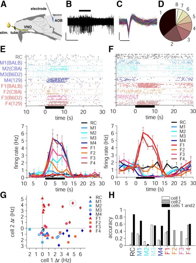
Recording from AOB and using responses of individual neurons to distinguish between stimuli. A, Experimental AOB recording setup: dilute urine from male and female mice of four different strains and Ringer's saline are delivered through a stimulus tube in random order to the VNO of the anesthetized female B6D2F1 mouse while AOB neuronal responses are recorded using 16 channel Neuronexus electrodes. B, Application of a urine stimulus to VNO for 10 s (horizontal black bar, top; female 129Sv urine) results in a neuronal firing rate increase in AOB. Calibration: 50 μV, 10 s. C, Single-unit neuronal spikes from complete recording, partially represented in B. Calibration: 50 μV, 1 ms. D, Proportion of neurons that responded to one or more stimuli. E, F, Raster plots (top) and peristimulus time histograms (bottom) of firing rate of two example cells in response to 10 s presentation of stimulus. The mean ± SD is shown. The stimulus naming convention is shown in D: strains BALB/c, CBA, B6D2, and 129Sv are renamed 1, 2, 3, and 4, respectively. The same convention applies in all subsequent figures. G, Firing rate responses, Δr, of two example neurons from E and F (here called Cell 1 and Cell 2, respectively) calculated over the 10 s stimulus presentation period. Each point is the Δr resulting from one stimulus repeat. Tight clustering of points for the same stimulus (e.g., red triangles, F1, female BALB/c urine) corresponds to a reliable response. On the other hand, high degree of scatter (e.g., red-orange squares, F2, female CBA urine) generally corresponds to high trial-to-trial variability. The circled point shows one of the five trials of female 129Sv urine (stimulus that yielded large responses in both neurons.) H, Stimulus classification accuracy of individual and combined cells 1 and 2, calculated using normalized Δr and the k nearest neighbors algorithm (see Materials and Methods). RC, Ringer's control.

Responses of individual neurons could often be used to partially distinguish among these stimuli. For example, for the neuron in Figure 1F, a strong excitatory response indicated that the urine stimulus was either from a female BALB/c or female 129Sv mouse; conversely, an inhibitory response indicated any one of the male urine stimuli, or female CBA. While these single-neuron responses were therefore somewhat informative, only a small minority of neurons (3 of 41) were selective for a single one of these stimuli (highest firing rate to one stimulus, distinct from all other stimuli; p < 0.05, Wilcoxon's rank-sum test), which are by themselves not different from Ringer's control. Thus, the large majority of responsive neurons produced responses that, on their own, were ambiguous.

Some of the ambiguities of single-neuron responses could be resolved by comparing responses across neurons. For example, the strong responses of the neuron in Figure 1F to female BALB/c and female 129Sv mice could be readily disambiguated by examining the responses of the cell in Figure 1E, which also responded strongly to female 129Sv, but not at all to female BALB/c. To approach this systematically, we computed the firing rate change from baseline, Δr, over the 10 s stimulus presentation period. Figure 1G shows the Δr, calculated for each individual trial of stimulus presentation, for these two neurons. If we imagine presenting a stimulus that yields large responses in both neurons (Fig. 1G, circled point), we could then use the closest examples of similar responses (a k nearest neighbors algorithm; see Materials and Methods) to deduce that this stimulus is likely from female 129Sv mice. Hence, by reference to the existing “templates” (which might correspond to previous sensory experience), one could rightly or wrongly classify any stimulus given the output of these two neurons. Because of trial-to-trial variability, it is apparent that not all eight stimuli can be perfectly disambiguated from each other and from the negative control. Nevertheless, two of the stimuli (female 129Sv and female BALB/c) could be recognized quite reliably, and for many of the remaining stimuli (for example, the samples from males), the combination of these two cells further reduces the ambiguity (Fig. 1H). On average, Cell 1 performed at 19% correct and Cell 2 at 29% correct. Combined, their performance grew to 48% correct. For three of nine stimuli (Ringer's control, male 129Sv, female BALB/c), the percentage correct was larger for the pair than for the sum of the two individual cells, providing clear evidence for multineuronal synergy.

The ability of two neurons to classify stimuli can naturally be extended to the entire population of recorded AOB neurons. The responses (Δr) of all cells in the population are shown in Figure 2A. Because we were not able to record from more than three responsive single-unit neurons simultaneously in one animal, we combined neurons that were recorded from different mice, assuming that the mice from the same strain, sex, and narrow age range were interchangeable (but see the following section). To better visualize the multineuronal representation of the different stimuli, we reduced the dimensionality of the data set by LDA to project population responses along a few highly informative axes.

By comparison with the two-cell case in Figure 1G, the projection of the population responses in two (Fig. 2B) and three (C) LDA dimensions greatly reduces the ambiguities among the sexes and strains. Most samples produced a set of tightly clustered responses for which the majority of neighbors were from the same sex and strain. A kNN algorithm (in five dimensions, four neighbors) led to an average accuracy of 82% across all eight urine stimuli. We analyzed the accuracy of the classifier for each stimulus, both in terms of the frequency with which it identified the correct stimulus and the frequency with which each incorrect choice was made. One sees that for all eight urine stimuli and the negative control, the mostly frequently chosen outcome was the correct one (Fig. 2D). The accuracy of the classification was not strongly dependent upon the number of neighbors used in the classifier, nor upon the number of dimensions (for three or more) used to project the data (Fig. 2E), indicating that success was largely independent of any particular choices for the classifier's parameters.

How many AOB neurons are required to perform this task? We explored this question using an iterative procedure, in which a group of “chosen” cells was augmented by incorporating the remaining cell that most improved the success rate (see Materials and Methods). This allowed us to plot the success rate as a function of pool size (Fig. 2F). One sees that the success rate rises to 80% within 11 cells, and reaches a near plateau of ∼90% within 18 cells, with a small drop-off at the end. Consequently, stimulus recognition can be performed accurately with only a modest subset of the full population. Thus, we conclude that neuronal population responses in the AOB suffice for accurate recognition of sex and strain.

Classification of stimuli by the VNO

The AOB receives its sensory input from the VNO, so a natural question is whether the raw vomeronasal sensory neuron (VSN) responses are equally informative, or whether the AOB might reshape VSN output to simplify this task. To address this question, we also recorded responses of VNO sensory neurons to these same dilute urine stimuli. Responses from female mouse VNO neurons were acquired using a 60 channel multielectrode array from Multichannel Systems. In total, we found 64 cells from VNO epithelia of 12 female B6D2F1 mice (aged 8–12 weeks) with reliable (p < 0.05, Wilcoxon's rank-sum test) change in firing rate (Arnson and Holy, 2011, 2013) to at least one stimulus (Fig. 3A).

Figure 3.

Classification of stimuli by the VNO. A, Firing rates of 64 VNO single units collected from female mice (n = 12) responsive to at least one stimulus at p < 0.05. B, Classification success rate as a function of cell pool size (k = 5, LDA dimensions 1–7). Black line, Success rate across all stimuli (4M+4F); blue line, success rate when distinguishing only among male urine stimuli (4M); red line, success rate when distinguishing only among female urine stimuli (4F). C, D, First two and three LDA projections of best 25 cells in the VNO data set. LD1, LD2, and LD3 are the LDA directions 1, 2, and 3, respectively. E, Classification result matrix (confusion matrix) for best 25 cells in the VNO [k = 5, LDA dimensions 1–7; vertical axis, patterns presented; horizontal axis, patterns predicted (classified)]. F, Classification matrix for all 64 cells. RC, Ringer's control.

Unlike the AOB, for the VNO we found that the success rate of classification was crucially dependent upon which cells were used by the classifier (Fig. 3B). In particular, the classification success was maximal for an intermediate number of cells (with the peak at 25 cells), and declined substantially when the entire population was used. To determine the origin of this difference between VNO and AOB, we first noted that the VSN population, when responsivity is judged by similar criteria used for the AOB, nevertheless contains a larger number of cells whose responses are weak (compare Figs. 2A, 3A). We therefore hypothesized that this declining success rate might be due to the difficulty in estimating the reliability of individual neurons from “just” five trials of each stimulus. To test this hypothesis, we performed recordings from a second set of five preparations in which each neuron was stimulated with 25 repeated trials of each stimulus (Fig. 4). We obtained a total of 87 stimulus-responsive (p < 0.05, Wilcoxon's rank-sum test) neurons, of which a similar proportion displayed responses that appeared quite weak. Like the five-trial experiments, we found that after the 10 best VNO cells were included, the resulting classification rate leveled off (here with ∼85–90% accuracy); however, in this case the success rate did not substantially diminish when the entire population was included. This indicates that, with 25 repeated presentations of each stimulus, the (un)reliability of cells could be accurately determined, and thus cells could be appropriately weighted when computing the best directions that separate the stimuli from our panel. This result indicates that this difference between VNO and AOB is a consequence of the lower signal-to-noise level of VSNs compared with AOB neurons (Meeks et al., 2010; Arnson and Holy, 2011).

Figure 4.

VNO, 25 presentations of each stimulus. A, Firing rate responses (Δr) of 87 single units recorded from n = 5 female B6D2F1 mice. Similar segregation of responses to male (M) and female (F) cues among the population of neurons as seen in Figure 3A. B, Varying k and number of dimensions to find the best parameters. Classification accuracy is not strongly dependent on the number of LDA dimensions used beyond 4, nor is it dependent on number of neighbors (k) used beyond 10. C, Classification success rate as a function of neuronal pool size (k = 11, 6 LDA dimensions). Black line, Success rate across all stimuli (4M+4F); blue line, success rate when distinguishing only among male urine stimuli (4M); red line, success rate when distinguishing only among female urine stimuli (4F). D, Three-dimensional LDA for best 44 cells. LD1, LD2, and LD3 are the LDA directions 1, 2, and 3, respectively. E, Confusion matrix for the best 44 cells. The color scale is the same as in F. F, Confusion matrix for all cells. For 25 repeats, the decline in accuracy is much less dramatic than for 5 repeats (compare Fig. 3E,F). RC, Ringer's control.

To examine the representation of these cues, we first focused on the best results, obtained with the subset of cells that gave the highest overall classification success (see Materials and Methods). Using these 25 best cells, we projected the population responses down to a few dimensions using LDA. In both two (Fig. 3C) and three dimensions, it is apparent that many of the responses to the different stimuli are readily distinguishable when using the responses of the neuronal population. As with the AOB, the kNN algorithm was able to identify an “unknown” stimulus from the population response with high accuracy, obtaining the correct answer the majority of the time for all nine types of stimuli. Overall, the classifier was correct 97% of the time (Fig. 3E).

To find out whether pooling of neurons from different mice had a major impact on our results, we performed the same analysis separately on several populations of simultaneously recorded neurons from single animals. In Figure 3A, Cells 20–28, 47–54, and 55–64 were recorded from VNOs of three different mice. Using these three sets of cells separately to classify the same set of urine stimuli yields the accuracy of 57, 55, and 70%, respectively. Choosing preparations that yielded a smaller number of responsive cells resulted in worse classification accuracy (for example, 36% for Cells 13–17, Fig. 3A); classification success was approximately linear in the number of neurons up to our largest population of 10 simultaneously recorded responsive neurons. Because of this result, and because mice have orders of magnitude higher numbers of VNO neurons that respond to urine, we do not expect that pooling neurons from multiple animals overestimates the classification capability of the neurons from a single animal.

To better understand the kinds of errors made when all cells (n = 64) satisfying our criterion for responsivity were used, we performed similar projections and classifications. We found that the accuracy in identification decreases, particularly for the samples from male mice (Fig. 3F). To determine the reason for this male/female difference, we measured the pairwise distance between the representation of all pairs of stimuli, using both a statistical classification measure, d′, and the correlation between population firing rate vectors. Using either measure, we find that pairs of samples from males excite responses that are closer and more highly correlated than those from females (Fig. 5A,B). This reflects higher similarity among VNO responses to male urine samples than to female urine samples (Figs. 3A, 4A). This does not hold for the responses measured in the AOB (Fig. 5C,D).

Figure 5.

Statistical measures of stimulus response similarity for neuronal ensembles. A, Left, Average across all cells of pairwise d′ values between cell Δr responses to stimuli in VNO; right, d′ is averaged across cells for all 6 possible pairs of male stimuli (-M), 6 pairs of female stimuli (-F), 16 pairs of male–female stimuli (M–F), 4 pairs of male–Ringer's (M–RC), and 4 pairs of female–Ringer's (F–RC). The mean ± SD is shown. B, Left, Pairwise correlations between neuronal ensemble responses to stimuli; right, correlation values averaged for the corresponding pairs of stimuli. C, Same as A, but for AOB. D, Same as B, but for AOB.

Consequently, we find that responses measured from both VNO and AOB can be used to achieve classification with low error rate, for both male and female cues. However, in VNO, one finds evidence that the task for male stimuli is more challenging than that for female stimuli. This is partially due to the fact that the differences among males appear to be more subtle than for females, as seen in Figure 5.

To determine whether the classification results are crucially dependent on the choice of classifier, we performed similar analyses using maximum likelihood inference (Dayan and Abbott, 2001). This classifier achieved a very similar success rate with similar numbers of neurons (Fig. 6). This demonstrates that these results generalize to a different classification algorithm.

Figure 6.

Distinguishing both sex and strain using maximum likelihood classifiers. A, Building up the VNO cell ensemble with two different classifiers: ML (green line) and LDA–kNN (black line, same as in Fig. 3B). B, Building up the AOB cell ensemble with two different classifiers: ML (green line) and LDA–kNN (black line, same as in Fig. 2F).

We also tested whether a more detailed representation of the responses—incorporating a measure of their temporal dynamics (Friedrich and Laurent, 2001; Stopfer et al., 2003)—improved accuracy. For these data, incorporating time did not yield greater accuracy (Fig. 7), presumably because any potential gains were canceled by the extra noise inherent in measuring responses over smaller time bins. Moreover, a PCA of the response time course (Fig. 7C,F) suggested that projections emphasizing the temporal evolution of responses (Fig. 7C, right) showed considerable overlap and little discriminability, whereas projections that collapsed much of the dynamics (C, left) were more informative. These results suggest that there is little or no advantage in taking the response time course into account, and that the rate code over the entire stimulus presentation period, roughly corresponding to the total spike count, is sufficient for decoding stimuli with high accuracy. This is consistent with AOS operating on temporal scales of seconds (Meredith, 1994).

Figure 7.

Using temporal dynamics of AOB and VNO neuronal firing to code for urine stimuli from males and females of different strains. A, Classification accuracy for AOB (n = 41 neurons, urine at 1:100 dilution in Ringer's) using binned firing rate independently and time bin size 2.5 s. Firing rates at time points denoted by green squares are used together in B. Stimulus is presented at time 0, lasting 10 s. Classification algorithm LDA followed by kNN is used (k = 4, dimensions 1–5, as in Fig. 2). Error bars indicate SD of accuracy after 10 iterations of the fivefold validation procedure. B, AOB classification accuracy of nine stimuli [including Ringer's control (RC)] using jointly the firing rates at four specific time points during the stimulus presentation cycle (marked by green squares in A). C, PCA of the time course of firing rate in AOB (mean across 5 stimulus trials) for the entire stimulus presentation cycle: 10 s on, 30 s Ringer's flush. The 40 s interval is divided into 16 time bins. Left and right panels show different aspects of the response time course trajectory: left, pattern trajectories separate into different “leaflets”; right, responses traverse ellipsoidal trajectories. D–F, Same analysis as in A–C, respectively, performed for VNO (n = 64 neurons, urine at 1:100 dilution in Ringer's, k = 5, dimensions 1–7 as in Fig. 3).

Classification with unknown concentration

Under natural circumstances, an animal exploring a stimulus may not have intrinsic knowledge about its concentration. However, until now these responses were measured with constant stimulus concentration, in which all urine stimuli were diluted 1:100. To explore the impact of variation in concentration on the ability to recognize individual stimuli, we performed a second set of recordings from both VNO and AOB using three different dilutions (1:100, 1:300, and 1:1000) of both female and male urine from two of the strains, BALB/c and CBA. We obtained 54 responsive neurons in the VNO, and 31 in the AOB.

Both VNO and AOB neurons tended to increase their firing rates with increasing concentration (Fig. 8A,B). LDA projections of both VNO and AOB in three dimensions show grouping of population responses according to stimulus identity, despite varying concentrations (Fig. 8C,D). When asked to judge the stimulus identity, independent of concentration, neuronal populations from both the VNO and AOB achieved a substantial degree of success (Fig. 8E,F).

Figure 8.

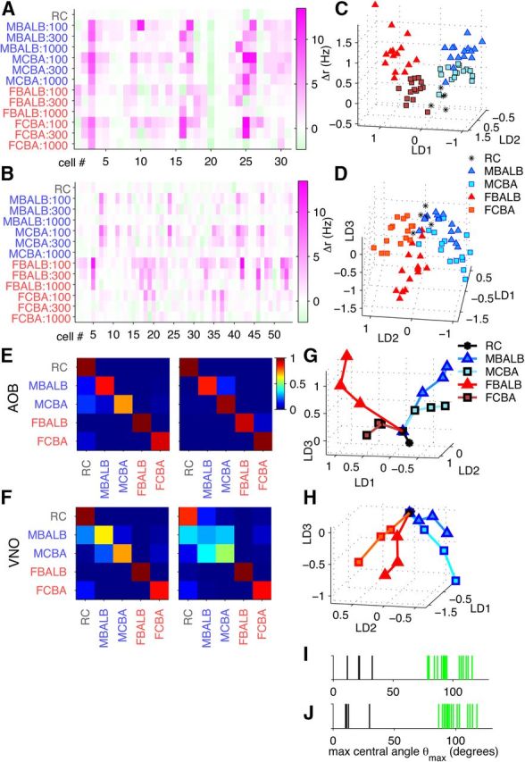
Concentration-invariant odor coding in AOB and VNO. A, AOB firing rate responses of 31 neurons to male and female BALB/c and CBA urine at three different dilutions (1:100, 1:300, and 1:1000). B, VNO firing rate responses of 54 neurons to the same urine stimuli at three different dilutions as in A. C, LDA projections of AOB responses at 1:100, 1:300, and 1:1000 stimulus dilutions intermixed. Each group, such as male BALB/c (MBALB), contains 15 points, 5 points at each dilution. D, LDA projections of VNO responses at dilutions 1:100, 1:300, and 1:1000. E, Classification accuracy matrix for AOB for the best 29 cells (left) and all 31 cells (right). F, Classification for VNO for the best 29 cells (left) and all 54 cells (right). G, H, Mean centroids for LDA projections of the best AOB (G) and VNO (H) cell responses for every stimulus at each of the three dilutions. Colored lines join points corresponding to the same stimulus. For every stimulus, making it more concentrated resulted in cell responses farther away from the origin in the LDA space. I, J, Maximum central angles θ_max for the original trajectories (black bars) and trajectories resulting from shuffled labels (green) at each dilution. The difference between distributions was assessed with Wilcoxon's rank-sum test: AOB, p = 0.003 (I); VNO, p = 0.003 (J). RC, Ringer's control; FBALB, female BALB/c; FCBA, female CBA; MCBA, male CBA.

To explore the origins of this success, we plotted the average population response to each stimulus and dilution, projecting down to a small number of dimensions (Fig. 8G,H). We found that different stimuli triggered population responses that emanated in different directions with increasing stimulus concentration. In general, the curves did not cross, and many traced out trajectories that were reasonably straight (Fig. 8I,J), as quantified with the maximum central angle (θ_max) measure (see Materials and Methods). This indicates that identity is at least partially decoupled from concentration, and presents one potential avenue for robust encoding of stimulus identity.

It is also apparent from these figures that the male cues are, particularly at lower concentrations, less distinct than the female cues, particularly for VNO. This is consistent with the reduced separation in VNO, even at a 1:100 dilution, of male stimuli compared to female stimuli (Fig. 5A,B).

We also tested the capacity of the neural population code to generalize to previously unseen stimulus concentrations. The dimensionality of the firing rate responses at one of the dilutions was reduced by LDA, as described above, and the resultant coding space LDA directions were stored. The firing rate responses at the two remaining dilution levels were projected onto the stored LDA directions and classified using the kNN algorithm. Training the AOB neuronal ensemble of 29 best cells at 1:1000 stimulus dilution and testing it at 1:300 dilution resulted in 92% accuracy; testing it at 1:100 resulted in 99% accuracy (Fig. 9A), which closely matches the result from testing and training at the same high 1:100 dilution. The VNO was slightly less robust at generalization: training the VNO neuronal ensemble of 29 best cells at 1:1000 and testing it at 1:300 resulted in an 80% accuracy, and testing it at 1:100 resulted in an 83% accuracy (Fig. 9B). This indicates that information from weak responses at low stimulus concentrations can be generalized to higher concentrations, with greater success in the AOB than in the VNO. Similarly, information from a high stimulus concentration can also be used to predict stimulus identity at a low concentration. For both VNO and AOB, training at 1:100 and testing at 1:300 and 1:1000 resulted in matching or better performance than that from testing and training at the same 1:300 and 1:1000 dilutions (Fig. 9).

Figure 9.

Concentration-invariant odor coding in AOB and VNO: training and testing on different dilutions. A, Train to classify male and female urine on two strains (BALB/c and CBA) at one dilution (for AOB). Resultant linear directions (LDs) from this dilution were used to test on the other two dilutions. Horizontal axis, Dilution of the test urine in Ringer's control (RC); vertical axis, classification accuracy. Black line (control), Train and test classifier at the same urine dilution. The horizontal position for some circles was shifted by a small amount to reduce overlap. B, Same as in A, but for VNO.

It is noteworthy that training on a spread of concentrations does not yield measureable benefits over training at a particular concentration and generalizing to higher or lower concentrations. This suggests that pattern recognition in the AOS may not rely on exposure to the same ligand at many different concentrations; instead, the nature of coding in this system results in “specific directions” in response space that may be associated with individual stimuli. These directions are quite stable over at least 10-fold changes in concentration.

Discussion

The accessory olfactory system in rodents detects and processes social olfactory cues to execute appropriate courtship and territorial responses. The natural compounds secreted in mouse urine are among the best-studied of these stimuli (Wyatt, 2003; Stowers and Marton, 2005; Brennan and Zufall, 2006). We used multielectrode recordings to systematically investigate the natural stimulus coding logic and robustness in neurons of the first two stages of accessory olfactory processing, the VNO and AOB. While several previous studies have looked at tuning specificity of individual neurons (Holy et al., 2000; Luo et al., 2003; He et al., 2008; Hendrickson et al., 2008; Holekamp et al., 2008; Nodari et al., 2008; Ben-Shaul et al., 2010), to our knowledge this is the first study to explicitly quantify the population decoding accuracy in AOB and VNO.

The majority of cells in both VNO (48 of 64, 75%) and AOB (26 of 41, 63%) were activated by urine stimuli from more than one mouse strain, suggesting that olfactory information could be encoded by combinatorial activation of the neurons. We have found that single-trial firing rate responses of a population consisting of a few well-chosen VNO and AOB neurons can be used to reliably encode both sex and strain information of a mouse urine donor. Using a k nearest neighbors algorithm to quantify discrimination accuracy, we found that the recognition of individual urine stimuli was well above chance level, at 80–90% for both AOB and VNO, with only 10 or so neurons necessary to reach this level. No single neuron could approach average classification accuracy of 50% by itself, confirming that it is necessary to use population activity (preferably of neurons with “complementary” tuning profiles) to decode stimulus information on a single-trial basis. Thus, the first two odor-processing stages in the AOS appear to encode sex-strain information with sufficient accuracy to make it feasible for the downstream brain regions to decode it. Previous work suggests that there may be sufficiently different features in urine from different individuals of the same strain and sex to provide a substrate for discrimination among individuals (Holy et al., 2000; He et al., 2008; Ben-Shaul et al., 2010), but the question of reliability has not been quantitatively addressed.

When comparing VNO to AOB, one notes that there is a change in neuronal representation of male and female urine stimuli. The block-diagonal appearance of the VNO correlation matrix stands in contrast with a more uniform appearance of the AOB correlation matrix, where there is substantial correlation between responses to males and to females. This can be explained by the observed nature of neuronal tuning in VNO and AOB. VNO neurons tend to increase their firing rate in response to either male urine or female urine, but rarely to both. No such overall segregation based on sex of the urine donor was observed in AOB, consistent with a role for at least some sensory integration in the AOB (Takami and Graziadei, 1990; Del Punta et al., 2002; Wagner et al., 2006; Yonekura and Yokoi, 2008; Meeks et al., 2010).

In the VNO but not the AOB, we found evidence that the task of discriminating among male urine cues is more challenging than that among female urine cues. This contrast is apparent when ensemble responses of all cells collected from the VNO are taken into account, as opposed to using just the best cells (Fig. 3B,E,F). As all VNO neurons were used, the accuracy in male strain identification decreased from 100 to ∼60%, whereas the female identification accuracy decreased from 100 to ∼95%. This finding is consistent with previous studies of the VNO (Stowers et al., 2002; He et al., 2008) that reported fewer cells responding to male urine than female urine and also smaller magnitude of response to male urine than female urine. In the AOB, however, no such imbalance has been reported (Hendrickson et al., 2008). We find that, on average, the diversity of VNO responses to male urine (as measured by pairwise d′ and correlation metrics; Fig. 5A,B) is smaller than that to female urine. The corresponding measures in the AOB are similar for male and female urine. Transformation of the olfactory input patterns from VNO to AOB appears to result in an increased relative separation between the representations of male patterns.

An animal must be able to discriminate between different odorants not only at one particular concentration, but also at different intensity levels. To test robustness of odor coding in the system, we challenged the AOB and VNO neuronal populations with three different dilution levels of four urine stimuli in Ringer's saline. In this test, the decoder had no knowledge of dilution factors, yet both AOB and VNO neurons encoded the stimulus identity with high accuracy. In a modified challenge, we tested the capacity of the neural population code to generalize to previously unseen stimulus concentrations. The decoder was trained at one dilution level and was able to successfully use the resultant principal directions in coding space to decode at the other two dilution levels. As seen in Figure 8, A and B, the firing rate responses tend to become smaller with progressively higher stimulus dilutions. Along with the results above, this serves to reject the notion that odor coding could be implemented in a static lookup table fashion, where different stimuli are recognized by employing a firing rate threshold or window. Instead, the accessory olfactory system appears to encode the stimulus identity by representing different stimuli as diverging paths in coding space.

An important future direction is to determine the impact, if any, of the hormonal status of the female subject on accessory olfactory function. In this study, the estrous status of the experimental subject was not controlled, and our results represent an average over different states. Female hormonal status influences olfactory behavior (Beach, 1976; Pierman et al., 2006; Wesson et al., 2006), although it is not clear that this reflects sensory function rather than downstream areas (Bressler and Baum, 1996). If discrimination accuracy does vary with the estrous cycle, then it seems likely that peak performance would be even higher than reported here, which would be an interesting topic for further mechanistic study.

We have seen that the AOB neuronal ensemble encodes sex and strain information with sufficient accuracy for decoding by a putative downstream brain region. In the accessory olfactory system, the majority of AOB projections are to the medial amygdala (MeA; Brennan, 2001). The MeA, as the downstream area of olfactory processing, likely represents odors in a way that is yet more salient to the animal. Investigating how and whether stimulus representation is transformed from AOB to MeA to aid the animal's behavioral decision making is a natural extension of current work.

References

- Arnson HA, Holy TE. Chemosensory burst coding by mouse vomeronasal sensory neurons. J Neurophysiol. 2011;106:409–420. doi: 10.1152/jn.00108.2011. [DOI] [PMC free article] [PubMed] [Google Scholar]
- Arnson H, Holy T. Robust encoding of stimulus identity and concentration in the accessory olfactory system. J Neurosci. 2013;33:13388–13397. doi: 10.1523/JNEUROSCI.0967-13.2013. [DOI] [PMC free article] [PubMed] [Google Scholar]
- Arnson H, Fu X, Holy T. Multielectrode array recordings of the vomeronasal epithelium. J Vis Exp. 2010:1845. doi: 10.3791/1845. [DOI] [PMC free article] [PubMed] [Google Scholar]
- Beach FA. Sexual attractivity, proceptivity, and receptivity in female mammals. Horm Behav. 1976;7:105–138. doi: 10.1016/0018-506X(76)90008-8. [DOI] [PubMed] [Google Scholar]
- Ben-Shaul Y, Katz LC, Mooney R, Dulac C. In vivo vomeronasal stimulation reveals sensory encoding of conspecific and allospecific cues by the mouse accessory olfactory bulb. Proc Natl Acad Sci U S A. 2010;107:5172–5177. doi: 10.1073/pnas.0915147107. [DOI] [PMC free article] [PubMed] [Google Scholar]
- Brennan PA. The vomeronasal system. Cell Mol Life Sci. 2001;58:546–555. doi: 10.1007/PL00000880. [DOI] [PMC free article] [PubMed] [Google Scholar]
- Brennan PA. The nose knows who's who: chemosensory individuality and mate recognition in mice. Horm Behav. 2004;46:231–240. doi: 10.1016/j.yhbeh.2004.01.010. [DOI] [PubMed] [Google Scholar]
- Brennan PA. Outstanding issues surrounding vomeronasal mechanisms of pregnancy block and individual recognition in mice. Behav Brain Res. 2009;200:287–294. doi: 10.1016/j.bbr.2008.10.045. [DOI] [PubMed] [Google Scholar]
- Brennan PA, Zufall F. Pheromonal communication in vertebrates. Nature. 2006;444:308–315. doi: 10.1038/nature05404. [DOI] [PubMed] [Google Scholar]
- Bressler SC, Baum MJ. Sex comparison of neuronal fos immunoreactivity in the rat vomeronasal projection circuit after chemosensory stimulation. Neuroscience. 1996;71:1063–1072. doi: 10.1016/0306-4522(95)00493-9. [DOI] [PubMed] [Google Scholar]
- Bruce HM. An exteroceptive block to pregnancy in the mouse. Nature. 1959;184:105. doi: 10.1038/184105a0. [DOI] [PubMed] [Google Scholar]
- Bruce HM, Parrott DM. Role of olfactory sense in pregnancy block by strange males. Science. 1960;131:1526. doi: 10.1126/science.131.3412.1526. [DOI] [PubMed] [Google Scholar]
- Dayan P, Abbott L. Theoretical neuroscience: computational and mathematical modeling of neural systems. Cambridge, MA: MIT; 2001. [Google Scholar]
- Del Punta K, Puche A, Adams NC, Rodriguez I, Mombaerts P. A divergent pattern of sensory axonal projections is rendered convergent by second-order neurons in the accessory olfactory bulb. Neuron. 2002;35:1057–1066. doi: 10.1016/S0896-6273(02)00904-2. [DOI] [PubMed] [Google Scholar]
- Døving KB, Trotier D. Structure and function of the vomeronasal organ. J Exp Biol. 1998;201:2913–2925. doi: 10.1242/jeb.201.21.2913. [DOI] [PubMed] [Google Scholar]
- Friedrich RW, Laurent G. Dynamic optimization of odor representations by slow temporal patterning of mitral cell activity. Science. 2001;291:889–894. doi: 10.1126/science.291.5505.889. [DOI] [PubMed] [Google Scholar]
- Halpern M. The organization and function of the vomeronasal system. Annu Rev Neurosci. 1987;10:325–362. doi: 10.1146/annurev.ne.10.030187.001545. [DOI] [PubMed] [Google Scholar]
- He J, Ma L, Kim S, Nakai J, Yu CR. Encoding gender and individual information in the mouse vomeronasal organ. Science. 2008;320:535–538. doi: 10.1126/science.1154476. [DOI] [PMC free article] [PubMed] [Google Scholar]
- Hendrickson RC, Krauthamer S, Essenberg JM, Holy TE. Inhibition shapes sex selectivity in the mouse accessory olfactory bulb. J Neurosci. 2008;28:12523–12534. doi: 10.1523/JNEUROSCI.2715-08.2008. [DOI] [PMC free article] [PubMed] [Google Scholar]
- Holekamp TF, Turaga D, Holy TE. Fast three-dimensional fluorescence imaging of activity in neural populations by objective-coupled planar illumination microscopy. Neuron. 2008;57:661–672. doi: 10.1016/j.neuron.2008.01.011. [DOI] [PubMed] [Google Scholar]
- Holy TE, Dulac C, Meister M. Responses of vomeronasal neurons to natural stimuli. Science. 2000;289:1569–1572. doi: 10.1126/science.289.5484.1569. [DOI] [PubMed] [Google Scholar]
- Luo M, Fee MS, Katz LC. Encoding pheromonal signals in the accessory olfactory bulb of behaving mice. Science. 2003;299:1196–1201. doi: 10.1126/science.1082133. [DOI] [PubMed] [Google Scholar]
- Macmillan N, Creelman C. Detection theory: a user's guide. New York: Psychology; 2005. [Google Scholar]
- Meeks JP, Arnson HA, Holy TE. Representation and transformation of sensory information in the mouse accessory olfactory system. Nat Neurosci. 2010;13:723–730. doi: 10.1038/nn.2546. [DOI] [PMC free article] [PubMed] [Google Scholar]
- Meredith M. Chronic recording of vomeronasal pump activation in awake behaving hamsters. Physiol Behav. 1994;56:345–354. doi: 10.1016/0031-9384(94)90205-4. [DOI] [PubMed] [Google Scholar]
- Meredith M. Human vomeronasal organ function: a critical review of best and worst cases. Chem Senses. 2001;26:433–445. doi: 10.1093/chemse/26.4.433. [DOI] [PubMed] [Google Scholar]
- Nodari F, Hsu FF, Fu X, Holekamp TF, Kao LF, Turk J, Holy TE. Sulfated steroids as natural ligands of mouse pheromone-sensing neurons. J Neurosci. 2008;28:6407. doi: 10.1523/JNEUROSCI.1425-08.2008. [DOI] [PMC free article] [PubMed] [Google Scholar]
- Papes F, Logan DW, Stowers L. The vomeronasal organ mediates interspecies defensive behaviors through detection of protein pheromone homologs. Cell. 2010;141:692–703. doi: 10.1016/j.cell.2010.03.037. [DOI] [PMC free article] [PubMed] [Google Scholar]
- Pierman S, Douhard Q, Balthazart J, Baum MJ, Bakker J. Attraction thresholds and sex discrimination of urinary odorants in male and female aromatase knockout (arko) mice. Horm Behav. 2006;49:96–104. doi: 10.1016/j.yhbeh.2005.05.007. [DOI] [PubMed] [Google Scholar]
- Quian Quiroga R, Panzeri S. Extracting information from neuronal populations: information theory and decoding approaches. Nat Rev Neurosci. 2009;10:173–185. doi: 10.1038/nrn2578. [DOI] [PubMed] [Google Scholar]
- Stopfer M, Jayaraman V, Laurent G. Intensity versus identity coding in an olfactory system. Neuron. 2003;39:991–1004. doi: 10.1016/j.neuron.2003.08.011. [DOI] [PubMed] [Google Scholar]
- Stowers L, Marton TF. What is a pheromone? Mammalian pheromones reconsidered. Neuron. 2005;46:699–702. doi: 10.1016/j.neuron.2005.04.032. [DOI] [PubMed] [Google Scholar]
- Stowers L, Holy TE, Meister M, Dulac C, Koentges G. Loss of sex discrimination and male-male aggression in mice deficient for TRP2. Science. 2002;295:1493–1500. doi: 10.1126/science.1069259. [DOI] [PubMed] [Google Scholar]
- Takami S, Graziadei PP. Morphological complexity of the glomerulus in the rat accessory olfactory bulb-a Golgi study. Brain Res. 1990;510:339–342. doi: 10.1016/0006-8993(90)91387-V. [DOI] [PubMed] [Google Scholar]
- Wagner S, Gresser AL, Torello AT, Dulac C. A multireceptor genetic approach uncovers an ordered integration of VNO sensory inputs in the accessory olfactory bulb. Neuron. 2006;50:697–709. doi: 10.1016/j.neuron.2006.04.033. [DOI] [PubMed] [Google Scholar]
- Wesson DW, Keller M, Douhard Q, Baum MJ, Bakker J. Enhanced urinary odor discrimination in female aromatase knockout (arko) mice. Horm Behav. 2006;49:580–586. doi: 10.1016/j.yhbeh.2005.12.013. [DOI] [PMC free article] [PubMed] [Google Scholar]
- Wyatt T. Pheromones and animal behaviour: communication by smell and taste. Cambridge, UK: Cambridge UP; 2003. [Google Scholar]
- Yonekura J, Yokoi M. Conditional genetic labeling of mitral cells of the mouse accessory olfactory bulb to visualize the organization of their apical dendritic tufts. Mol Cell Neurosci. 2008;37:708–718. doi: 10.1016/j.mcn.2007.12.016. [DOI] [PubMed] [Google Scholar]